Symmetric Triple Well with Non-Equivalent Vacua: Instantonic Approach

Abstract

We show that for the triple well potential with non-equivalent vacua, instantons generate for the low lying energy states a singlet and a doublet of states rather than a triplet of equal energy spacing. Our energy splitting formulae are also confirmed numerically. This splitting property is due to the presence of non-equivalent vacua. A comment on its generality to multi-well is presented.

PACS numbers: 31.15.Kb; 03.65.Xp; 03.65.Ge.
Keywords: Instanton; Non-perturbative effect; Bound states; Path integral method.

Instantons are non-trivial classical solutions of Euclidean field equations for which the action is finite [1]. Their importance, besides being topological configurations, comes from their finite contributions to Feynmann path integral. In quantum mechanics instantons correspond to non-trivial finite classical solutions of classical equations of motion with inverted potential [2].

The uses of instanton calculations have proven to be useful in analyzing non-perturbative aspects of quantum mechanical systems with degenerate vacua, this is because instanton solutions contribute to the quantum tunnelling phenomena, which can be calculated with the aid of the dilute gas approximation. A celebrated example is the splitting of energy level in the symmetric double well case [2].

To our knowledge only a few recent papers attempted to apply the instanton method to the triple well potential with non-equivalent vacua [3, 4, 5]. This problem is rather involved compared to the symmetric double well case. It has been suspected that in the presence of non-equivalent vacua the dilute gas approximation may break down [5]. Moreover it has been claimed[3, 4] that the average of the harmonic frequencies over the non-equivalent vacua of the potential serves as the central position for the equidistant nearly degenerate first three levels. Unfortunately this claim does not lead to the correct spectra and is in contradiction with the numerical calculations. Thus understanding the structure of the energy levels in a triple well becomes important. These issues encourage us to look at the problem more carefully and to our knowledge a proper treatment has not been previously carried out.

In this work, we consider the triple well potential of the form, which admits inversion symmetry $(x\rightarrow-x)$,

$$V(x)={\omega^{2}\over 2}\,x^{2}\,(x^{2}-1)^{2},$$ (1)

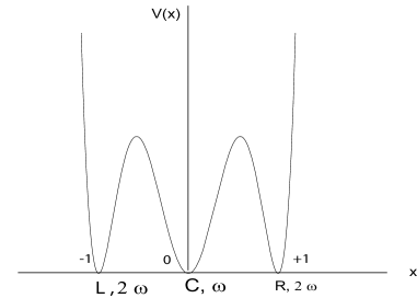
Figure 1: Triple well: $V(x)={\omega^{2}\over 2}\,x^{2}\left(x^{2}-1\right)^{2}$

The potential ,$V(x)$, shown in Fig. 1 consists of central, left and right well separated by barriers. In the vicinity of each well (near the minima at $x=0,\pm 1$) the potential can be approximated as a harmonic oscillator potential. The frequency corresponding to the central well is $\omega_{0}=\omega$, while for the left and right well is $\omega_{1}=2\,\omega$ as can be easily verified by expanding the potential around each minima. These different frequencies show the different curvatures at each minima.

Computation of transition probability amplitudes between different minima allows to extract the low lying energy eigenvalues. Here the instanton contributions to these transitions are calculated by making a proper treatment for the non-equivalent vacua. As will be shown this proper treatment has a drastic effect on the energy spectra in contrast with what has been claimed.

For the potential in Eq. (1) we have four kinds of instanton solutions connecting neighboring minima and have the forms:

$$x^{I}(t)=\pm{1\over\left[1+e^{\mp\omega\left(t-t_{0}\right)}\right]^{{1\over 2}}} x^{\bar{I}}(t)=\pm{1\over\left[1+e^{\pm\omega\left(t-t_{0}\right)}\right]^{{1\over 2}}},$$ ,

(2)

where $I(\bar{I})$ indicates instanton(anti-instanton) respectively.

The transition from the minimum at $x=0$ to that at $x=1$ during the Euclidean time interval $T$ can be written as:

$$\langle 1|e^{-HT}|0\rangle=\langle 1|E_{0}\rangle\,\langle E_{0}|0\rangle\;e^{-E_{0}\,T}+\langle 1|E_{2}\rangle\,\langle E_{2}|0\rangle\;e^{-E_{2}\,T}\;+\cdots$$ (3)

Due to the symmetry only even states contribute (odd states are vanishing at $x=0$). On the other hand for the transition from $x=1$ to $x=1$, we have

$$\langle 1|e^{-HT}|1\rangle=|\langle 1|E_{0}\rangle|^{2}\;e^{-E_{0}\,T}+|\langle 1|E_{1}\rangle|^{2}\;e^{-E_{1}\,T}+|\langle 1|E_{2}\rangle|^{2}\;e^{-E_{2}\,T}\;+\cdots$$ (4)

These transitions, Eqs. (3)-(4), are sufficient to extract the low lying energy eigenvalues namely $E_{0},E_{1}$ and $E_{2}$.

In the dilute gas approximation, a typical instantonic contribution to the transition in Eq. (3) is found to be composed of $i+1$ instantons and $i$ anti-instanton as shown in Fig. 2 which we call, for later use, $M_{i}^{\mbox{odd}}$.

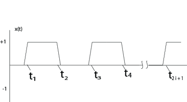
Figure 2: The multi instanton contribution to the transition from $x=0$ to $x=1$. The solutions with positive slope are called instantons whereas those of negative are called anti-instanton

It should be stressed that this contribution has $2^{i}$ different configurations which should be taken into consideration during calculations.

For the case of the transition, Eq. (4), one finds that it is composed of $i-$instantons and $i$ anti-instantons as shown in Fig. 3 which we call $M_{i}^{\mbox{even}}$. This contribution has $2^{i-1}$ different configurations. Also there is a contribution coming from the trivial solution $(x(t)=1)$ that should be taken into consideration.

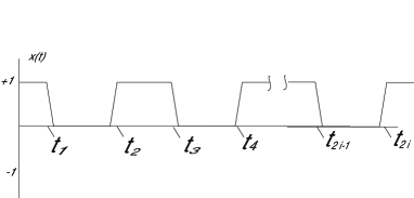
Figure 3: The multi instanton contribution to the transition from $x=1$ to $x=1$. The solutions with positive slope are called instantons whereas those of negative are called anti-instanton

It is worthy to note the following remarks. Firstly, in evaluating the transition drawn in Figs. (2,3) we have to compute the fluctuations over these paths consisting of strings of instantons-anti-instantons. However, because instantons are quite localized (with extension of order $\omega^{-1}$), we can neglect the fluctuations around their bodies. In other words, the quantum fluctuations would be effective only around the straight line paths in Figs. (2,3). Along each step of the straight line paths, the particle resides at the minima of the potential (maxima for the inverted one) shown in Fig. 1. These fluctuations can be treated like the case of the harmonic oscillator. The crucial point here is to take care that the frequencies corresponding to each step may be different and can not be taken to be equal. Secondly, to compute the transition probability amplitudes given by Eqs. (3)-(4) one should sum over all the possible multi-instanton-anti-instanton configurations. An elegant method for avoiding this complicated sum has been developed and implemented in Refs. [6, 7] to the case of quantum mechanical system with degenerate classical minima (exemplified by the symmetric double well) giving correct results for the low lying energy spectra and also non trivial information about the wave functions. The method in Refs. [6, 7] is based on saturating the transition probability amplitudes from the minimum to itself by the trivial solution, while for the transitions between two successive minima by one-instanton. However to extract energy eigenvalues one should have a priori some knowledge about the pattern of the correct energy spectra. Since in our present work we do not have such a priori knowledge about the correct pattern for the energy spectra for the symmetric triple well with non-equivalent vacua, thus the sum over the multi-instanton-anti-instanton configurations can not be avoided.

Using a technique similar to that used for the double well with non-equivalent vacua [8], we rearrange the n-instanton integrals in such a form that recursive relations can be given for all these integrals. With the help of these relations the instanton sum can be easily managed. As stated before, only two transitions are required to be calculated, namely that between the minima at $x=0$ and $x=1$ and the other between $x=1$ to $x=1$.

The contribution of the $M_{i}^{\mbox{odd}}$ has the integral:

$$M_{i}^{\mbox{odd}} = 2^{i}\,NK^{2\,i+1}A^{2\,i+1}\int_{-{T\over 2}}^{{T\over 2}}dt_{1}\;\int_{t_{1}}^{{T\over 2}}dt_{2}\cdots\cdots\int_{t_{2\,i}}^{{T\over 2}}\,dt_{2\,i+1}$$

$$e^{-{1\over 2}\omega_{0}(t_{1}-(-{T\over 2}))}\;e^{-{1\over 2}\omega_{1}(t_{2}-t_{1})}\;e^{-{1\over 2}\omega_{0}(t_{3}-t_{2})}\cdots e^{-{1\over 2}\omega_{1}({T\over 2}-t_{2\,i+1})},$$

$$= 2^{i}NK^{2\,i+1}A^{2\,i+1}\;e^{-{1\over 2}{\omega_{0}+\omega_{1}\over 2}T}\;\int_{-{T\over 2}}^{{T\over 2}}dt_{1}\;\int_{t_{1}}^{{T\over 2}}dt_{2}\cdots\cdots\int_{t_{2\,i}}^{{T\over 2}}\,dt_{2\,i+1}$$

$$e^{\delta\,t_{1}}\,e^{-\delta\,t_{2}}\,e^{\delta\,t_{3}}\cdots e^{\delta\,t_{2\,i+1}},$$

where $(\,N=\sqrt{{\omega\over 2\,\pi}}\,)$ is the normalization constant, $A$ is the exponential of the classical Euclidean action for one instanton and $\delta={\omega_{1}-\omega_{0}\over 2}$. The factor $K$ is calculated by matching the one instanton contribution. The one instanton contribution for the potential ,Eq. (1), can be found in Refs. [3, 4], but with paying attention to used different conventions.

Now this integral can be put in an equivalent form:

$$M_{i}^{\mbox{odd}}={N\over\sqrt{2}}\,B^{2\,i+1}\,e^{-{1\over 2}{\omega_{0}+\omega_{1}\over 2}T}\;\int_{-{T\over 2}}^{{T\over 2}}\;dt\;e^{\delta t}\,{({T\over 2}+t)^{i}\over i!}\,{({T\over 2}-t)^{i}\over i!},$$ (6)

where $B=\sqrt{2}\,K\,A$ .

For the transition from $x=1$ to $x=1$, the corresponding integral is

$$M_{i}^{\mbox{even}} = 2^{i-1}\,NK^{2\,i}A^{2\,i}\int_{-{T\over 2}}^{{T\over 2}}dt_{1}\;\int_{t_{1}}^{{T\over 2}}dt_{2}\cdots\cdots\int_{t_{2\,i-1}}^{{T\over 2}}\,dt_{2\,i}$$

$$e^{-{1\over 2}\omega_{1}(t_{1}-(-{T\over 2}))}\;e^{-{1\over 2}\omega_{0}(t_{2}-t_{1})}\;e^{-{1\over 2}\omega_{1}(t_{3}-t_{2})}\cdots e^{-{1\over 2}\omega_{1}({T\over 2}-t_{2\,i})},$$

$$= N2^{i-1}\,K^{2\,i}A^{2\,i}\;e^{-{\omega_{1}\over 2}T}\;\int_{-{T\over 2}}^{{T\over 2}}dt_{1}\;\int_{t_{1}}^{{T\over 2}}dt_{2}\cdots\cdots\int_{t_{2\,i-1}}^{{T\over 2}}\,dt_{2\,i}$$

$$e^{-\delta\,t_{1}}\,e^{\delta\,t_{2}}\,e^{-\delta\,t_{3}}\cdots e^{\delta\,t_{2\,i}},$$

(7)

which can also be put in an another equivalent form

$$M_{i}^{\mbox{even}}={N\over 2}B^{2\,i}\,e^{-{1\over 2}{\omega_{0}+\omega_{1}\over 2}T}\;\int_{-{T\over 2}}^{{T\over 2}}\;dt\;e^{\delta t}\;{({T\over 2}+t)^{i-1}\over(i-1)!}\,{({T\over 2}-t)^{i}\over i!}.$$ (8)

Carrying out the sum over the multi-instantons is rather involved, but can be simplified by studying the basic integral of the form

$$I(n,m)=B^{n+m+1}\,e^{-{1\over 2}{\omega_{0}+\omega_{1}\over 2}T}\;\int_{-{T\over 2}}^{{T\over 2}}\;dt\;e^{\delta t}\,{({T\over 2}+t)^{n}\over n!}\,{({T\over 2}-t)^{m}\over m!}.$$ (9)

Integrating by parts we get the following recursive relations (here we drop the common factor $e^{-{1\over 2}{\omega_{0}+\omega_{1}\over 2}T}$ in the definition of $I(n,m)$)

$$I(n,0) = {B\over\delta}\,\left[{(B\,T)^{n}\over n!}\,e^{\delta\,{T\over 2}}-I(n-1,0)\right],$$

$$I(0,m) = {B\over\delta}\,\left[I(0,m-1)-{(B\,T)^{m}\over m!}\,e^{-\delta\,{T\over 2}}\right],$$

$$I(n,m) = {B\over\delta}\,\left[I(n,m-1)-I(n-1,m)\right].$$

With the help of these recursive relations, Eqs. (LABEL:rec1), and taking into account the correct counting together with the starting initial integral $I(0,0)={B\over\delta}\,\left[e^{\delta\,{T\over 2}}-e^{-\delta\,{T\over 2}}\right],$ we get (here we keep the common factor in the definition of $I(n,m)$)

$$I(n,m) = e^{-{1\over 2}\omega_{0}\,T}\sum_{i=0}^{n}\left(\begin{array}[]{c}m+n-i\\ m\end{array}\right)(-1)^{n-i}\;\left({B\over\delta}\right)^{n+m-i+1}\,{(B\,T)^{i}\over i\,!}$$ (13)

$$+ e^{-{1\over 2}\omega_{1}\,T}\sum_{j=0}^{m}\left(\begin{array}[]{c}m+n-j\\ n\end{array}\right)(-1)^{n+1}\;\left({B\over\delta}\right)^{n+m-j+1}\,{(B\,T)^{j}\over j\,!},$$ (16)

where $(^{\,m}_{\,n})$ are the binomial coefficients.

For the transition from the minimum at $x=0$ to the one at $x=1$ we need to evaluate the sum $\sum_{i=0}^{\infty}\,I(i,i)$ which is still hard to perform using Eq. (LABEL:bas2). To facilitate evaluating the sum, we define $S(n,m)=\sum_{i=0}^{\infty}\,I(n+i,m+i)$ and let $S^{\pm}_{j}(n,m)$ be the coefficient of $S(n,m)$ associated with the terms ${(B\,T)^{j}\over j!}\,e^{\pm\,{\delta\,T\over 2}}$. Using the recursion relations, Eqs. (LABEL:rec1), one gets

$$S_{i}^{\pm}(n,m) = {B\over\delta}\left[S_{i}^{\pm}(n,m-1)-S_{i}^{\pm}(n-1,m)\right],$$

$$S_{i}^{+}(n,m) = S_{i+1}^{+}(n+1,m),$$

$$S_{i}^{-}(n,m) = S_{i+1}^{-}(n,m+1),$$

$$S_{i}^{+}(n,m) = S_{i}^{+}(i,m+i-n)\;\;\;\mbox{where n $<$ i},$$

$$S_{i}^{-}(n,m) = S_{i}^{-}(n+i-m,i)\;\;\;\mbox{where m $<$ i}.$$

By letting $a_{i}^{\pm}\equiv S_{i}^{\pm}(i,i)$, then with the aid of the recursion relations, Eqs.(LABEL:rec2), we get

$$a_{i+1}^{\pm}=a_{i-1}^{\pm}\mp{\delta\over B}\,a_{i}^{\pm},$$ (19)

consequently the sum over the multi-instantons becomes

$$\sum_{i=0}^{\infty}\,M_{i}^{\mbox{odd}}={N\over\sqrt{2}}\,\sum_{i=0}^{\infty}\,I(i,i)={N\over\sqrt{2}}\,\sum_{i=0}^{\infty}\,\left(a^{+}_{i}\,{(B\,T)^{i}\over i!}\,e^{-\,{\omega_{0}\,T\over 2}}+a^{-}_{i}\,{(B\,T)^{i}\over i!}\,e^{-\,{\omega_{1}\,T\over 2}}\right).$$ (20)

The coefficient $a^{+}_{i}$ corresponds to the coefficient of linear combination of two exponential (note that the factorial factor is removed) namely that

$$C_{+}\,e^{\alpha_{+}}+C_{-}\,e^{\alpha_{-}},$$ (21)

where $\alpha_{\pm}$ are found to be

$$\alpha_{\pm}=-{\delta\over 2B}\pm\,\sqrt{\left({\delta\over 2B}\right)^{2}+1}.$$ (22)

The coefficients $C_{+}$ and $C_{-}$ can be then determined from

$$a_{0}^{+} = C_{+}\,+C_{-},$$

$$a_{1}^{+} = C_{+}\,\alpha_{+}\,+C_{-}\,\alpha_{-},$$

$$= C_{+}\,\left(-{\delta\over 2B}+\,\sqrt{\left({\delta\over 2B}\right)^{2}+1}\;\right)$$

$$+ C_{-}\,\left(-{\delta\over 2B}-\,\sqrt{\left({\delta\over 2B}\right)^{2}+1}\;\right).$$

Thus from Eq. (LABEL:bas2) we get

$$a_{0}^{+}=\sum_{i=0}^{\infty}\,\left(\begin{array}[]{c}2\,i\\ i\end{array}\right)(-1)^{i}\,\left({B\over\delta}\right)^{2\,i+1}={B\over\delta}{1\over\sqrt{1+\left({2B\over\delta}\right)^{2}}}={1\over 2\sqrt{1+\left({\delta\over 2B}\right)^{2}}},$$ (24)

and

$$a_{1}^{+}=\sum_{i=1}^{\infty}\,\left(\begin{array}[]{c}2\,i-1\\ i\end{array}\right)(-1)^{i-1}\,\left({B\over\delta}\right)^{2\,i}={1\over 2}-{1\over 2}\,{1\over\sqrt{1+\left({2B\over\delta}\right)^{2}}}.$$ (25)

leading to $C_{+}={1\over 2\sqrt{1+\left({\delta\over 2B}\right)^{2}}}$ and $C_{-}=0$. A similar treatment can be done for $a_{i}^{-}$ leading to the results $C_{-}=-{1\over 2\sqrt{1+\left({\delta\over 2B}\right)^{2}}}$ and $C_{+}=0$. Using these results together with Eq. (20), one finally obtains for the odd multi-instantons sum:

$$\sum_{i=0}^{\infty}\,M_{i}^{\mbox{odd}}={N\over 2\,\sqrt{2}\,\sqrt{1+\left({\delta\over 2B}\right)^{2}}}\left[e^{-E_{0}\,T}-e^{-E_{1}\,T}\right],$$ (26)

with

$$E_{0} = {(\omega_{0}+\omega_{1})\over 4}-\sqrt{{\delta^{2}\over 4}+B^{2}},$$

$$E_{2} = {(\omega_{0}+\omega_{1})\over 4}+\sqrt{{\delta^{2}\over 4}+B^{2}}.$$

Now the transition probability amplitude between the minimum at $x=1$ to itself, after including the contribution of the trivial solution $(x(t)=1)$, becomes

$$\langle 1|e^{-H\,T}|1\rangle=N\,e^{-{\omega_{1}\,T\over 2}}+\sum_{i=1}^{\infty}\,M_{i}^{\mbox{even}}=N\,e^{-{\omega_{1}\,T\over 2}}+{N\over 2}\,\sum_{i=1}^{\infty}\,I(i-1,i),$$ (28)

which can be evaluated by the same procedure applied for the transition between the minimum at $x=0$ to that at $x=1$. For this purpose we let $\Lambda_{i}^{\pm}=S_{i}^{\pm}(i,i+1)$ where $S_{i}^{\pm}(i,i+1)$ defined as before. Using the recursion relations in Eqs. (LABEL:rec2) we obtain

$$\Lambda^{+}_{i}={B\over\delta}\left[\Lambda^{+}_{i-1}-\Lambda^{+}_{i+1}\right],$$ (29)

The coefficient $\Lambda^{+}_{i}$ corresponds to the coefficient of linear combination of two exponential (note that the factorial factor is removed) namely that

$$D_{+}\,e^{\lambda_{+}}+D_{-}\,e^{\lambda_{-}},$$ (30)

where $\lambda_{\pm}$ are found to be

$$\lambda_{\pm}=-{\delta\over 2B}\pm\,\sqrt{\left({\delta\over 2B}\right)^{2}+1}.$$ (31)

The coefficients $D_{+}$ and $D_{-}$ can be then determined from

$$\Lambda_{0}^{+} = D_{+}\,+D_{-},$$

$$\Lambda_{1}^{+} = D_{+}\,\lambda_{+}\,+D_{-}\,\lambda_{-},$$

$$= D_{+}\,\left(-{\delta\over 2B}+\,\sqrt{\left({\delta\over 2B}\right)^{2}+1}\;\right)$$

$$+ D_{-}\,\left(-{\delta\over 2B}-\,\sqrt{\left({\delta\over 2B}\right)^{2}+1}\;\right).$$

Again using Eq. (LABEL:bas2) we get

$$\Lambda_{0}^{+}=\sum_{i=1}^{\infty}\,\left(\begin{array}[]{c}2\,i-1\\ i\end{array}\right)(-1)^{i-1}\,\left({B\over\delta}\right)^{2\,i}={1\over 2}-{1\over 2\sqrt{1+\left({\delta\over 2B}\right)^{2}}},$$ (33)

and

$$\Lambda_{1}^{+} = \sum_{i=2}^{\infty}\,\left(\begin{array}[]{c}2\,i-2\\ i\end{array}\right)(-1)^{i-2}\,\left({B\over\delta}\right)^{2\,i-1},$$

$$= {4\left({B\over\delta}\right)^{3}\over\sqrt{1+\left({2B\over\delta}\right)^{2}}\left(1+\sqrt{1+\left({2B\over\delta}\right)^{2}}\right)^{2}}\,,$$

which from Eqs. (LABEL:sol3) lead to $D_{+}={1\over 2}-{1\over 2}{1\over\sqrt{1+\left({\delta\over 2B}\right)^{2}}}$ and $D_{-}=0$. A similar treatment can be done for $\Lambda_{i}^{-}=S_{i-1}^{-}(i-1,i)$ leading to the recursive relation

$$\Lambda^{-}_{i}={B\over\delta}\left[a^{-}_{i-1}-\Lambda^{-}_{i-1}\right].$$ (38)

After a lengthy algebra we finally get the instantonic contribution

$$\sum_{i=1}^{\infty}I(i-1,i) = \left({1\over 2}-{1\over 2}\,{1\over\sqrt{1+\left({2B\over\delta}\right)^{2}}}\right)\,e^{-E_{0}\,T}$$

$$- e^{-E_{1}\,T}+\left({1\over 2}+{1\over 2}\,{1\over\sqrt{1+\left({2B\over\delta}\right)^{2}}}\right)\,e^{-E_{2}\,T},$$

where $E_{0}$ and $E_{2}$ as before, while $E_{1}={\omega_{1}\over 2}$.

To sum up we finally get our formulae for the energy spectra for the triple well, arranged in ascending order from the ground state,:

$$E_{0} = {(\omega_{0}+\omega_{1})\over 4}-\sqrt{{\delta^{2}\over 4}+B^{2}},$$

$$E_{1} = {\omega_{1}\over 2},$$

$$E_{2} = {(\omega_{0}+\omega_{1})\over 4}+\sqrt{{\delta^{2}\over 4}+B^{2}},$$

where $B$ for the potential in Eq. (1) is: ${8\over\sqrt{3\,\pi}}\,\omega^{3/2}\,e^{-{\omega\over 4}}$.

Our formulae, Eqs. (LABEL:ener2), are completely different from that of Refs. [3, 4]. In the limit of large $\omega$, the spectra tend to the limit $E_{0}\rightarrow{\omega\over 2}$, $E_{2}\rightarrow E_{1}=\omega$, i.e. a singlet and a degenerate doublet.

To confirm our formulae we resort to numerical solution of Schr$\ddot{o}$dinger equation for the potential Eq. (1). In this letter we present the results for the energy differences in Table 1 and for the individual energy eigenvalues in Table 2. The details of the numerical method can be found in Ref. [9]. Moreover our results are consistent with what one could predict based on simple quantum mechanical approach to the problem Ref. [10].

$\omega$	$\Delta E_{10}^{\mbox{\it num}}$	$\Delta E_{10}^{\mbox{\it ins}}$	$\Delta E_{21}^{\mbox{\it num}}$	$\Delta E_{21}^{\mbox{\it ins}}$
$30$	$13.67878984$	$15.00373814$	$0.004723029$	$0.003738143$
$50$	$23.77967090$	$25.00000047$	$9.100602755\,\times 10^{-7}$	$4.715381063\,\times 10^{-7}$
$70$	$33.81102645$	$35.00000000$	$1.018592013\,\times 10^{-10}$	$4.195754855\,\times 10^{-11}$
$90$	$43.82678307$	$45.00000000$	$8.950392428\,\times 10^{-15}$	$3.552713679\,\times 10^{-15}$
$110$	$53.83629393$	$55.00000000$	$6.844874590\,\times 10^{-19}$	$2.135638335\,\times 10^{-19}$

Table 1: The numerically calculated energy differences ($\Delta E^{\mbox{\it num}}$) against those ($\Delta E^{\mbox{\it ins}}$) predicted using instantonic approach. Notice that $\Delta E_{ij}=E_{i}-E_{j}$.

	$\omega=30$	$\omega=50$	$\omega=70$
$E_{0}$	$14.178009913879056439$	$24.211602974742920912$	$34.22366585434764411968736$
$E_{1}$	$27.856799752355288816$	$47.991273870020627020$	$68.03469230180201792058325$
$E_{2}$	$27.861522781409804929$	$47.991274780080902476$	$68.03469230190387712184547$

	$\omega=90$	$\omega=110$
$E_{0}$	$44.229945163238886600375384901$	$54.233802436877662843887532359$
$E_{1}$	$88.056728233456712807586843449$	$108.070096366408926121501688376$
$E_{2}$	$88.056728233456721757979271787$	$108.070096366408926122186175835$

Table 2: The numerically calculated energy eigenvalues. Numerical results, for large $\omega$, show singlet and doublet structures ($E_{0}\rightarrow{\omega\over 2}$, $E_{2}\rightarrow E_{1}=\omega$).

In this letter we have emphasized the power of the application of the instanton method, when a proper treatment is used, and shown that the dilute gas approximation is sufficient. We have confirmed our splitting energy formulae numerically. As a final comment we expect that for a potential well with non-equivalent vacua, the multiplicity of the splitting is related to the number of equivalent vacua connected by the discrete symmetry of the potential.

References

• [1] G. ’t Hooft, Phys. Rev. Lett. 37, (1976) 8 ; Phys. Rev. D 14, (1976) 3432 .
• [2] S. Colemann, Aspects of Symmetry, Cambridge Univ. Press (1985).
• [3] S. Y. Lee et al., Mod. Phys. Lett. A 12, (1997) 1803 .
• [4] J. Casahorr$\acute{a}$n, Phys. Lett. A 283, (2001) 285 .
• [5] M. Sato and T. Tanaka, J. Math. Phys. 43, (2002) 3484 .
• [6] G. C. Rossi and M. Testa, Ann. Phys. (NY) 148, (1983) 144.
• [7] F. Cesi, G. C. Rossi and M. Testa, Ann. Phys. (NY) 206, (1991) 318.
• [8] A. Rivero quant-ph/0209072.
• [9] H. A. Alhendi and E. I. Lashin quant-ph/0305128, submitted to Can. J. Phys.
• [10] H. A. Alhendi and E. I. Lashin quant-ph/0406075.