Adiabatic and non-adiabatic merging of independent Bose condensates

Abstract

Motivated by a recent experiment [Chikkatur et al. Science, 296, 2193 (2002)] on the merging of atomic condensates, we investigate how two independent condensates with random initial phases can develop a unique relative phase when we move them together. In the adiabatic limit, the uniting of independent condensates can be understood from the eigenstate evolution of the governing Hamiltonian, which maps degenerate states (corresponding to fragmented condensates) to a single state (corresponding to a united condensate) . In the non-adiabatic limit corresponding to the practical experimental configurations, we give an explanation on why we can still get a large condensate fraction with a unique relative phase. Detailed numerical simulations are then performed for the non-adiabatic merging of the condensates, which confirm our explanation and qualitative estimation. The results may have interesting implications for realizing a continuous atom laser based on merging of condensates.

I Introduction

The prospect of the creation of a continuous, coherent atomic beam, the atomic analogy of laser beam, has been of great interest to many ever since the successful generation of Bose-Einstein condensate (BEC) 1 ; 2 ; 16 ; 3 ; 13 ; 14 ; 15 ; 17 . One of the major challenges to such applications lies in the difficulty in continuous condensation of atomic gas due to stringent cooling conditions. Towards that goal, one needs to spatially separate the evaporative cooling from the destructive laser cooling, which is still pretty challenging even though there’ve been interesting investigations and progresses 17 ; 18 ; 19 . Alternatively, one can realize a continuous source of condensate by bringing new condensates into the trap and uniting them. Note that independently prepared condensates have a completely random relative phase; in order to unite them, one needs to have a phase cooling mechanism to get rid of this random phase. Interesting theoretical investigations have been carried out on the possibilities of uniting two existing condensates through laser induced phase cooling with condensates confined in a high-Q ring cavity 4 , or through phase locking with feedbacks from a series of interference measurements 5 .

Recently, Chikkatur et al. reported a striking experiment in which two independently produced condensates were merged directly in space by bringing their traps together to a complete overlap6 . A condensate fraction larger than the initial components was observed from the subsequent time-of-flight imaging. This raises the question as how the relative phase between the two component condensates is established during this direct merging where there is no additional phase cooling or locking. In this paper, we investigate this puzzling phase dynamics both in the ideal adiabatic merging limit and in the more practical non-adiabatic circumstance. In the ideal adiabatic limit, we show that a unique relative phase will be established between the two components during direct merging, resulting from the eigenstate evolution of the governing Hamiltonian (an effective two-mode model). The Hamiltonian has degenerate ground states corresponding to two fragmented condensates when the traps are apart. When we overlap the two traps, the degenerate ground states evolve into a single eigenstate corresponding to a single condensate with a unique relative phase between the two initial components. While the adiabatic limit requires very slow merging, the real experiment is actually performed far from that limit 6 . In this case, the atoms will slip from the ground state to all the nearby eigenstates, and one would not expect to get a single condensate. However, through a careful analysis of the eigenstate structure of the governing Hamiltonian, we argue that one can still get a large condensate fraction (larger than either of the initial components’) with a unique relative phase in this non-adiabatic limit. We then confirm this evolution picture through detailed numerical simulations of the merging dynamics.

We should also point out that the non-adiabatic merging considered in this paper, which is based on the parameters of the experiment 6 , is not an abrupt connection of the two condensates. In the latter case, a unique relative phase cannot be established without careful consideration of dissipation 7 . In the experiment, the time scale of the merger( 0.5 s) is long when compared with the trap frequency (440Hz) along the merging direction6 . So the merging is actually adiabatic with respect to the evolution of the condensate wave packets; and dissipation due to the quasi-particle excitation in each well should not play an important role. However, this same merging time scale is very short when compared with the lowest excitation energy of the relevant Hamiltonian (the effective two-mode model). Many eigenstates of this Hamiltonian will get populated during the merger. That is why we call it ”non-adiabatic”. Our central observation is that due to the particular eigen-energy distribution of this relevant two-mode Hamiltonian, even for mergers much faster than the lowest excitation energy, only low-lying states of the Hamiltonian will be populated. Furthermore, for all the populated low-lying states, the relative phase between the two initial condensate components is well locked. As a result, we will get a large merged condensate fraction with a uniquely established relative phase.

In the following, we first present a theoretical model for the description of the direct merging process, and argue that the internal phase dynamics is mainly captured by the simplified two-mode Hamiltonian with time dependent parameters, which has been a popular model for many theoretical investigations in different scenarios 7 ; 8 ; 9 ; 10 ; 11 ; 12 . After that, we go to the main topic and investigate the relative phase dynamics. The result in the adiabatic limit can be easily understood. In the non-adiabatic limit, the arguments need to be based on the analysis of the detailed evolution structure of the eigenstates of the time-dependent Hamiltonian. Then in Sec. III, we investigate the relative phase dynamics and the evolution of the condensate fraction through detailed numerical simulations, with the evolution speed ranging from the adiabatic limit to the far non-adiabatic circumstance. We simulate the merging process with different configurations and different initial states of the two components. Finally, we discuss the relevance of the results to the reported experiment and to the prospect of producing continuous atom lasers based on condensate merging.

II Theoretical modeling of adiabatic and non-adiabatic merging of independent condensates

II.1 An effective two-mode model for the description of the relative phase dynamics

Consider two independently prepared condensates in separate traps at low temperature. The two traps are then brought closer along a certain direction to allow the condensates to merge, as illustrated in Fig. 1. The traps can be modeled as a time-dependent double-well potential $V_{T}(\mathbf{r},t)$, with the two wells moving towards each other. The interactions between the atoms are described by the usual $\delta$-pseudopotential, $U(\mathbf{r_{1},r_{2}})=(4\pi\hbar a_{s}/m)\delta(\mathbf{r_{1},r_{2}})$, where $a_{s}$ is the s-wave scattering length and $m$ is the mass of the atom. The second quantization Hamiltonian for such a system has the form

$$\hat{H} = \int\hat{\Psi}^{{\dagger}}(\mathbf{r})(\frac{P^{2}}{2m}+V_{T}(\mathbf{r},t))\hat{\Psi}(\mathbf{r})d\mathbf{r}$$ (1)

$$+\frac{g}{2}\int\hat{\Psi}^{{\dagger}}(\mathbf{r})\hat{\Psi}^{{\dagger}}(\mathbf{r})\hat{\Psi}(\mathbf{r})\hat{\Psi}(\mathbf{r})d\mathbf{r},$$

where $\hat{\Psi}\left(r\right)$ is the bosonic quantum field operator describing the atoms, and the parameter $g=4\pi\hbar a_{s}/m$.

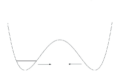
Figure 1: Illustration of merging of two independent condensates.

When the traps are not overlapping, the atoms in the same condensate are in the same quantum mode. We can expand the atomic field operator $\hat{\Psi}(\mathbf{r})$ as $\hat{\Psi}(\mathbf{r})=a_{1}\phi_{1}(\mathbf{r})+a_{2}\phi_{2}(\mathbf{r}),$, where $\phi_{i}(\mathbf{r})$ $\left(i=1,2\right)$ are the corresponding mean-fields from the Gross-Pitaevski equation for each trap. When we bring the two condensates closer by varying the trap potential $V_{T}(\mathbf{r},t)$, we assume that the atomic density profile adiabatically follows the movement of the traps, as is the case in the experiment6 . With this assumption, at any given time $t$, we can still use a variational mean field $\phi_{i}(\mathbf{r,t})$ to describe the corresponding condensate. The condensate wave functions now overlap in space, and the atoms in different condensates can tunnel to each other through the trap barrier. As a good approximation, we can expand the atomic field $\hat{\Psi}(\mathbf{r,t})$ at time $t$ as $\hat{\Psi}(\mathbf{r,t})=a_{1}\phi_{1}(\mathbf{r,t})+a_{2}\phi_{2}(\mathbf{r,t})$. With this expansion, the Hamiltonian (1) is simplified to the following well-known two-mode model

$$\hat{H}=\frac{U\left(t\right)}{4}\left(a_{2}^{{\dagger}}a_{2}-a_{1}^{{\dagger}}a_{1}\right)^{2}-\frac{J\left(t\right)}{2}(a_{1}^{{\dagger}}a_{2}+a_{2}^{{\dagger}}a_{1}),$$ (2)

where the parameters $U\left(t\right)$ and $J\left(t\right)$ are given by

$$U(t)=\frac{g}{2}\int(\left|\phi_{1}\right|^{4}+\left|\phi_{2}\right|^{4}-2\left|\phi_{1}\right|^{2}\left|\phi_{2}\right|^{2})d\mathbf{r},$$ (3)

$$J(t)=-2\int\phi_{1}^{\ast}(\frac{P^{2}}{2M}+V(\mathbf{r},t))\phi_{2}d\mathbf{r}.$$ (4)

In writing Eq. (2), we have assumed a symmetric trap with $\int\left|\phi_{1}\right|^{4}d\mathbf{r}=\int\left|\phi_{2}\right|^{4}d\mathbf{r}$, and we have neglected terms that are functions only of the atom number $\hat{N}$, as they commute with $\hat{H}$ and can be eliminated by going to a rotating frame. We have also neglected the nonlinear tunneling terms proportional to $(a_{1}^{{\dagger}}a_{2}+a_{2}^{{\dagger}}a_{1})^{2}$ (see Ref. 10 for the coefficient before that term) because they are either typically smaller than or have the same effect as the linear tunneling, so that neglecting them does not change the basic physics 21 . Note that given all the approximations above, the factor before the last term in Eq. (3) has some arbitrariness as this term is on the same order of magnitude as some neglected terms in the weak overlapping limit. As a convenient choice, we take the factor to be $2$ so that we have a vanishing $U(t)$ as the two traps completely overlap, as one would expect on physical grounds. The two-mode Hamiltonian (2), which is a very popular model for many theoretical investigations in different scenarios 7 ; 8 ; 9 ; 10 ; 11 ; 12 , catches the main physics of condensates in double-well potentials resulting from the competition between the tunneling and the local nonlinear collision interaction. A more detailed and more rigorous derivation of the two-mode model from the variational approximation can be found in Ref. 12 . One important limitation for applications of the two-mode model is that when the two condensates get very close, the coupling between the two condensates becomes so strong that some approximations underlying the two-mode model are not well justified. In that strong overlapping region, Eqs. (2)-(4) serve as a convenient extrapolation. However, numerical calculation reveals that the relative phase and the condensate fraction are established shortly after the commencement of the merger, when the two condensates are not yet strongly coupled. It is under this context that we think an effective two-mode model catches the main physics and is adequate for the understanding of the relative phase evolution.

We will use the time-dependent two-mode model (Hamiltonian (2)) to investigate the relative phase dynamics during the merging of independent condensates. The temporal behavior of the coefficients $U\left(t\right)$ and $J\left(t\right)$ in principle should be derived from the self-consistent variational solutions of $\phi_{1}(\mathbf{r,t})$ and $\phi_{2}(\mathbf{r,t})$, which is pretty involved. Fortunately, in the following we will see that the relative phase dynamics is actually insensitive to the details of $U\left(t\right)$ and $J\left(t\right)$. It only depends on the rough scale of their rates of variation. Hence, for the following discussions in this section, we do not specify the explicit forms of $U\left(t\right)$ and $J\left(t\right)$. Nevertheless, we do know the rough trends of the evolutions of $U\left(t\right)$ and $J\left(t\right)$. As the two traps approach each other, $J\left(t\right)$ will continuously increase from zero to a maximum value $J_{0}$. Compared with $J(t)$, $U\left(t\right)$ typically changes much more slowly at the beginning of the merger, and can be roughly taken as a constant $U_{0}.$ As the two traps further merge approaching to a complete overlap, one expects that $U\left(t\right)$ will gradually decrease to zero. These rough trends of evolutions of $U\left(t\right)$ and $J\left(t\right)$ are important for the understanding of the relative phase dynamics.

II.2 Merging of condensates in the adiabatic limit

For the convenience of the following discussions, we write the two-mode model (2) using effective collective spin operators. With the standard Schwinger representation of the spin operators $\hat{S}_{x}=\frac{1}{2}(a_{1}^{{\dagger}}a_{2}+a_{2}^{{\dagger}}a_{1})$, $\hat{S}_{y}=\frac{i}{2}(a_{1}^{{\dagger}}a_{2}-a_{2}^{{\dagger}}a_{1})$, and $\hat{S}_{z}=\frac{1}{2}(a_{2}^{{\dagger}}a_{2}-a_{1}^{{\dagger}}a_{1})$, Hamiltonian (2) can be expressed in the following form

$$\hat{H}\left(t\right)=U\left(t\right)\hat{S}_{z}^{2}-J\left(t\right)\hat{S}_{x}.$$ (5)

This Hamiltonian is actually equivalent to that of the infinite-range Ising model 20 , and one has effective anti-ferromagnetic interaction as $U\left(t\right)>0$.

First, let us assume that the temperature of the atoms is low enough, and that the variation speeds of $U\left(t\right)$ and $J\left(t\right)$ are very small. In this ideal adiabatic limit, the establishment of a unique relative phase through direct merging of condensates can be easily understood from the adiabatic theorem, which states that the system in such a limit will remain in the ground state of the Hamiltonian $\hat{H}\left(t\right)$. Initially, the two traps are far apart, therefore the self interaction among the atoms in each trap dominates with $U\left(t\right)\rightarrow U_{0}$ and $J\left(t\right)\rightarrow 0$. The ground state in this case is an eigenstate of $\hat{S}_{z}^{2}$ with eigenvalue of $0$, i.e., with $\left\langle a_{2}^{{\dagger}}a_{2}\right\rangle=\left\langle a_{1}^{{\dagger}}a_{1}\right\rangle=N/2$, where $N$ is the total atom number. The two condensates have equal number of atoms, but there is no phase relation between them, which corresponds to fragmented condensates. In the final stage of the merger, the coefficients $U\left(t\right)\rightarrow 0$ and $J\left(t\right)\rightarrow J_{0}$, the coupling energy $-J\left(t\right)\hat{S_{x}}$ thus dominates in the Hamiltonian. The ground state in this case is an eigenstate of $\hat{S}_{x}$ with the largest eigenvalue $N/2$ (without loss of generality we assume $J\left(t\right)>0$). This state is actually an eigenstate of the number operator $a_{+}^{\dagger}a_{+}$ of the mode $a_{+}=\left(a_{1}+a_{2}\right)/\sqrt{2}$ with an eigenvalue of $N$, which corresponds to a single condensate. We then have a unique zero relative phase between the two initial condensate modes $a_{1}$ and $a_{2}$, which is due to the fact that the coupling energy $-J\left(t\right)\hat{S_{x}}$ is minimized only when we have the same phase between $a_{1}$ and $a_{2}$.

The above understanding of the relative phase establishment from the adiabatic theorem seems to be simple and straightforward, but in a sense it is pretty nontrivial. The relative phase really comes from a joint effect of the two competitive terms in the Hamiltonian (5). If we have only the collision interaction term $U\left(t\right)\hat{S}_{z}^{2}$ and start with fragmented condensates with $\left\langle a_{2}^{{\dagger}}a_{2}\right\rangle=\left\langle a_{1}^{{\dagger}}a_{1}\right\rangle=N/2$, it’s obvious that the condensate fractions will never be changed by this collision interaction. On the other hand, if we have only the coupling term $-J\left(t\right)\hat{S_{x}}$, it will only rotate the two condensate modes $a_{1}$ and $a_{2}$ to two different modes $a_{1}^{\prime}$ and $a_{2}^{\prime}$, and will never change the condensate fractions either. The condensate fractions can be quantitatively described by the eigenvalues of the following single-particle density matrix 12

$$\rho=\left(\begin{array}[]{cc}\left\langle a_{1}^{{\dagger}}a_{1}\right\rangle&\left\langle a_{1}^{{\dagger}}a_{2}\right\rangle\\ \left\langle a_{2}^{{\dagger}}a_{1}\right\rangle&\left\langle a_{2}^{{\dagger}}a_{2}\right\rangle\end{array}\right).$$ (6)

The system is in a single-condensate state if $\rho$ has only one macroscopic eigenvalue in the limit $N\rightarrow\infty$; and it corresponds to fragmented condensates if $\rho$ has more macroscopic eigenvalues in the large $N$ limit. It is clear that the coupling term $-J\left(t\right)\hat{S_{x}}$ only makes a linear rotation of the modes $a_{1}$ and $a_{2}$, and will never change the eigenvalues of the single-particle density matrix $\rho$. Clearly, it is the interplay between these two competing interactions in the Hamiltonian (5) that is really responsible for producing a larger condensate fraction with a well-defined relative phase.

The analysis above gives us a simple understanding of how a unique relative phase in principle could be established between two initially independent condensates through direct merging in the perfect adiabatic limit. However, this analysis hardly explains the merging dynamics in real experiments because the practical configurations are far from this ideal adiabatic limit. Practically, first of all, we can never start with an equal number state for the two condensates. One can at most control the number of atoms in each condensate so that they are roughly the same, as each condensate has some number fluctuations typically on the order of $\sqrt{N}$. So in reality we can not start from the ground state of the Hamiltonian (5), but rather a statistical mixture of some low-lying states. Secondly, to fulfill the conditions of the adiabatic passage, one requires that the variation speeds of $U\left(t\right)$ and $J\left(t\right)$ be significantly smaller than the smallest eigen-frequency splitting of the relevant Hamiltonian. The Hamiltonian (5) has an energy difference of $U_{0}$ between the ground and the first excited state when $U\left(t\right)\gg J\left(t\right)$ (i.e., when the traps are far apart). This is a tiny energy gap, which can be roughly estimated by $\mu_{c}/N$, where $\mu_{c}$ denotes the chemical potential of the condensate ($\sim 2$kHz 21 ) and the atom number is typically around $10^{6}$. The merging time scale in real experiments ($\sim 0.5$ s 6 ) is much shorter than the time scale given by $1/U_{0}$. This shows that we need to go beyond the adiabatic limit to understand the merging dynamics in practical configurations, which is the focus of our next subsection.

II.3 Merging of condensates in the practical non-adiabatic circumstance

If the evolution speed of the Hamiltonian is beyond the adiabatic limit, the system prepared in the ground state will be excited to some upper eigenstates. The excitation probability will depend on the ratio of the variation rate of the Hamiltonian to the smallest energy difference between the two eigenstates 23 . The final state in this case is in general a superposition of different low-lying eigenstates which have been populated during the merger. Therefore, to find out the final state of the system in the non-adiabatic circumstance, it is important to look at the evolution of all the eigenstates of the Hamiltonian (5) during the merging process.

We have calculated the energy spectrum of the Hamiltonian (5) as a function of the ratio of $J\left(t\right)/U\left(t\right)$ for various atom numbers up to a few hundred (see also Ref. 24 , where the energy spectrum is drawn for other purposes). The evolutions of the energy spectrum for different atom numbers are qualitatively very similar. To have a clear display, we only plot in Fig. 2 the whole energy spectrum of the Hamiltonian (5) with a small atom number $N=20$, as the energy levels become too dense to be seen clearly in a small figure if $N$ is large. Fig. 2 is enough to show some general properties of the energy spectrum which are critical for the understanding of the merging dynamics outside of the adiabatic limit. The spectrum can be divided into three regions, corresponding respectively to the Fock, the Josephson, and the Rabi region, as discussed in general Josephson physics 21 . First of all, on the left side of the spectrum ($J\left(t\right)\rightarrow 0$), which corresponds to the Fock region, there are a total of $N+1$ eigenlevels. While the lowest eigenlevel ($j=0$) stays non-degenerate, the $\left(2j-1\right)$th and $\left(2j\right)$th ($j=1,2,\cdots,N/2$) levels are degenerate in energy. The two degenerate states can be expressed as $\left|N/2+j,N/2-j\right\rangle$ and $\left|N/2-j,N/2+j\right\rangle$ in the Fock basis of the modes $a_{1}$ and $a_{2}$ . The energy difference between the ground state and the $2j$th eigenlevel is given by $j^{2}U\left(t\right)\approx j^{2}U_{0}$. The quadratic scaling of the energy difference with $j$ is very important for the following discussions. Secondly, on the far right side of the spectrum with $J\gg NU$ (not shown in Fig. 2), the system enters the Rabi region, where the eigenlevels are almost equally spaced. In that region, one can approximately neglect the term $U\left(t\right)J_{z}^{2}$, and the energy levels are roughly eigenstates of the $\hat{S_{x}}$ operator. The $j$th ($j=0,1,2,\cdots N$) eigenlevel, expressed as $\left|S=N/2,S_{x}=N/2-j\right\rangle$ in the Dicke basis of the collective spin operator $\overrightarrow{S}$, has the energy $jJ\left(t\right)\approx jJ_{0}$ (compared with the ground state). Between these two limiting cases, there is a wide intermediate Josephson region where the two-mode model could be understood semi-classically 21 . In the Josephson region, with fixed $J$ and $U$, the energy levels for the low eigenstates are also approximately equally spaced with the energy difference between the adjacent levels given by $\sqrt{NUJ}$.

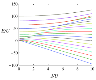
Figure 2: (Color Online) Energy spectrum of the Hamiltonian (5) with the atom number N=20 24 .

From the discussions above, we see that the Fock region has the smallest energy spacing for the low-lying eigenstates with typical experimental parameters. The non-adiabatic transition therefore happens dominantly in or close to that region. However, due to the quadratic scaling of the energy spacing in that region, although non-adiabatic transition occurs, the atoms can only be excited to some low-lying eigenstates if they start from the ground state. The typical merging time in the experiment 6 is about $0.5$ s, significantly longer than the time scale of $\hbar/\mu_{c}$, where $\mu_{c}$ ($\sim 2$kHz) is the chemical potential. The parameters $NU_{0}$ and $\mu_{c}$ are roughly on the same order of magnitude for typical atomic gas experiments. In the Fock region, the energy spacing between the $2\sqrt{N}$th excited state and the ground state is $NU_{0}$. So if the atoms start from the ground state, the final spread in the energy eigenstates due to the non-adiabatic transition is at most $2\sqrt{N}$. Of course, in real experiments it is not practical to start exactly from the ground state $\left|N/2,N/2\right\rangle$ of the Hamiltonian (5) when the traps are far apart. Let us assume that the initial atom numbers $N_{1}$ and $N_{2}$ in the two traps are roughly the same with $N_{1}\simeq N_{2}\simeq N/2$ 22 , and that each of them has some fluctuations typically on the order of $\sqrt{N}$ 25 . Then, the initial spread in the energy eigenlevel is about $2\sqrt{N}$. Adding together quadratically the contributions from the non-adiabatic transfer and from the initial number fluctuations , we conclude that after the merger, the atoms will populate a mixture of the low-lying eigenstates of the Hamiltonian (5), with a spread in the eigenstates characterized by $2\sqrt{2N}$ (in terms of the order of magnitude).

Now we want to show that even if the final state after the merger is a mixture of low-lying eigenstates, as long as the spread in the eigenstates $2\sqrt{2N}\ll N$, we still have a large single-condensate fraction. When the two traps are merged and we are in the Rabi region, we can calculate the condensate fraction in the mode $a_{c}=\left(a_{1}+a_{2}\right)/\sqrt{2}$ for each eigenstate of the $\hat{S_{x}}$ operator. For the $j$th eigenstate $\left|S=N/2,S_{x}=N/2-j\right\rangle$ of the $\hat{S_{x}}$ operator, its population in the mode $a_{c}$ is given by $N-j$ (This result can be easily seen if we rotate $\hat{S_{x}}$ to $\hat{S_{z}}$ through a linear transformation on the modes $a_{1}$ and $a_{2})$. Now we are in a mixture of the eigenstates $\left|S=N/2,S_{x}=N/2-j\right\rangle$ of the $\hat{S_{x}}$ operator with $j$ up to $2\sqrt{2N}$. For this mixture state, the atom number in the particular mode $a_{c}$ is at least $N-2\sqrt{2N}$. Therefore, if the atom number $N$ is huge, we end up with the dominant fraction of atoms in the mode $a_{c}$ even if the merging is far outside the perfect adiabatic limit. The basic reason for this result lies in the fast growth of the excitation energy with the levels. The system is kept in some low-lying states of the Hamiltonian (5) although the evolution is non-adiabatic. When most of the atoms are in the condensate mode $a_{c}$, a unique relative phase of zero is correspondingly established between the two initial modes $a_{1}$ and $a_{2}$.

III Numerical Simulation of the merging dynamics of two condensates

III.1 Numerical simulation methods

In the previous sections, we have shown that through a direct merger it is possible to establish a unique relative phase between two initially independent condensates, and argued that this relative phase is robust and we can almost get a single condensate even if the merging is far outside the adiabatic limit ($t_{m}\ll\hbar/U_{0}$). In this section, we would like to quantitatively test this result through more detailed numerical simulations of the merging dynamics.

To quantitatively describe the merging dynamics, we look at the evolution of the largest condensate fraction derived from the single-particle density matrix (6). The largest eigenvalue of the single-particle density matrix $\rho$ can always be expressed as an expectation value $\left\langle a_{c}^{\dagger}a_{c}\right\rangle$, where $a_{c}$ is a rotated mode corresponding to the largest condensate fraction and is defined as $a_{c}=\cos\theta a_{1}+\sin\theta e^{i\varphi}a_{2}$. The rotation angle $\theta$ reflects the contributions to the new condensate mode $a_{c}$ from the two initial modes $a_{1}$ and $a_{2}$, and $\varphi$ specifies their relative phase in this new mode. With this characterization of the relative phase, here we ignore explicit discussion on the inherent quantum uncertainty of the phase operator caused by the finite total atom number. This quantum uncertainty is on the order of $1/\sqrt{N}$, where the atom number $N\sim 10^{6}$ for typical experiments, so it represents a small effect. We refer the readers to Ref. phase for detailed discussions on that issue. Numerically, we start with certain initial states of the modes $a_{1}$ and $a_{2}$, as will be detailed in the following subsections, solve the evolution of these states under the Hamiltonian (5), and calculate the single-particle density matrix for each instantaneous state to find out the evolution of the atom number $\left\langle a_{c}^{\dagger}a_{c}\right\rangle$ in the largest condensate fraction mode $a_{c}$ and the corresponding parameters $\theta$ and $\varphi$. The atom number $\left\langle a_{c}^{\dagger}a_{c}\right\rangle$ is given by the largest eigenvalue of $\rho$, while $\theta$ and $\varphi$ are specified by the corresponding eigenvector $(\cos\theta,\sin\theta e^{i\varphi})$.

To quantify the state evolution, we need to specify the parameters $U\left(t\right)$ and $J\left(t\right)$ in the Hamiltonian (5) as a function of time. To be consistent with the experimental configurations in Ref. (13), we assume that the two initial condensates are confined in cigar-shaped traps which are moving towards each other along the radial direction with uniform speed. As we have mentioned before, the details of the functions $U\left(t\right)$ and $J\left(t\right)$ are not important, but rather their time scales. So, for simplicity, we assume that the wave functions $\phi_{i}(\mathbf{r,t})$ $\left(i=1,2\right)$ of the modes $a_{i}$, which adiabatically follow the movement of the cigar-shaped traps, also have cigar-shaped profiles specified by the following Gaussian function

$$\phi_{i}(\mathbf{r,t})=\frac{1}{\pi^{3/4}\sigma_{\rho}\sqrt{\sigma}_{z}}\exp\left[-\frac{\left[x-x_{i0}\left(t\right)\right]^{2}+y^{2}}{2\sigma_{\rho}^{2}}\right]$$

$$\times\exp\left[-\frac{z^{2}}{2\sigma_{z}^{2}}\right],\hskip 99.58464pt$$ (7)

where $\sigma_{\rho}$ and $\sigma_{z}$ are the widths of the wave functions along the radial and the axial directions, respectively. The centers of the wavepackets are given by $x_{10}(t)=x_{0}\left(1-t/t_{m}\right)/2$ and $x_{20}(t)=-x_{0}\left(1-t/t_{m}\right)/2$, defining a constantly diminishing separation from $x_{0}$ to $0$ throughout the merging time $t_{m}$. The variation of the parameters $U\left(t\right)$ and $J\left(t\right)$ are then calculated with Eqs. (3)(4) from these postulated wave functions. The typical evolution of $U\left(t\right)$ and $J\left(t\right)$ are shown in Fig. 5(a-b) with $\sigma_{z}=10\sigma_{\rho}$, following the experimental conditions 6 . Although in real experiments the total atom number is normally on the order of $\sim 10^{6}$, in numerical simulations, due to the limited computation speed, we can only deal with moderate atom numbers with $N\sim 10^{2}$. However, we know that $NU_{0}$ and $J_{0}$ are typically on the same order of magnitude with $J_{0}$ somewhat smaller than $NU_{0}$. In order to be consistent with the practical configurations, we should re-scale the parameters $U\left(t\right)$ and $J\left(t\right)$ with a global constant so that $NU_{0}\sim J_{0}$. In our simulation, without loss of generality, we assume $NU_{0}=4J_{0}$. When $U\left(t\right)$ and $J\left(t\right)$ are specified, we can numerically calculate the evolution of the atom number $\left\langle a_{c}^{\dagger}a_{c}\right\rangle$ in the largest condensate fraction and the relative phase $\varphi$ with the method described above.

III.2 Merging of two condensates in Fock states

We first investigate the merging of two condensates in Fock states, with the atom numbers $N_{1}=51$ and $N_{2}=49$, respectively. The numerical results are shown in Figs. (3a)-(3h), where the largest condensate fraction $\eta$ (defined as $\eta=\left\langle a_{c}^{\dagger}a_{c}\right\rangle/N$ with $N=N_{1}+N_{2}$) and the parameters ($\theta$,$\varphi$) are plotted against the dimensionless time $U_{0}t$. Note that for the initial Fock state, the relative phase $\varphi$ is not well defined (random). In the numerical program, one basically randomly picks up a particular initial phase. In Fig. 3, the initial value of $\varphi$ is set to zero simply due to the convention of the program (it sets phase $\varphi=0$ for the complex number $0e^{i\varphi}$). The merging dynamics and the final relative phase do not depend on this particular choice. We test other assignments of the initial phase, and basically there are no changes in the dynamics (except for different initial jumps of the phase which are meaningless). We have different merging time scales for figures (a)-(h), ranging from the adiabatic limit $U_{0}t_{m}=40$ to the complete non-adiabatic limit $U_{0}t_{m}=0.04$, where $t_{m}$ denotes the time of the merger. With $U_{0}t_{m}=40\gg 1$, the picture of the adiabatic mapping is basically valid, and as expected, finally we have more than $95\%$ of atoms evolving into the largest condensate fraction (see Fig. 3g). For Figs. (3e) and (3c), the time scales change from $U_{0}t_{m}=4$ to $U_{0}t_{m}=0.4$, which is certainly outside the adiabatic limit as $U_{0}t_{m}\lesssim 1$. However, since $NU_{0}t_{m}=100U_{0}t_{m}\gg 1$, as we analyzed in Sec. IIC, only some low-lying eigenlevels will be populated during the evolution, and we should have a good condensate fraction. This is confirmed by the figures (3e) and (3c). Compared with Fig. (3g), the final condensate fraction is reduced a little bit, but not much, in particular for Fig. (3e) with $NU_{0}t_{m}\gg 1$. Finally, in Fig. (3a) the variation is so fast ($NU_{0}t_{m}=4$) that many of the eigenlevels of the Hamiltonian (5) will be populated and we expect to have a poor final condensate fraction. This is confirmed by the numerical simulation, where we can hardly see any considerable increase of the condensate fraction.

Figures. (3b) (3d) (3f) and (3h) show the evolution of the corresponding condensate mode which has the largest fraction of the atoms. For Figs. (3d) (3f) and (3h), we expect that the final state should be close to the lowest eigenstate of the operator $-\hat{S}_{x}$. The corresponding condensate mode should be $a_{c}\simeq\left(a_{1}+a_{2}\right)/\sqrt{2}$, with $\theta\rightarrow\pi/4$ and $\varphi\rightarrow 0$. Indeed, we can see from these three figures that the parameters $\theta$ and $\varphi$ approach their stationary values with very small oscillations as soon as $J\left(t\right)$ becomes comparable to $U\left(t\right)$. When $J\left(t\right)\sim U(t)$, the system is well inside the Josephson region. This means that a unique relative phase has been established between the two initial modes $a_{1}$ and $a_{2}$ when their coupling is still weak. In such a region, the two-mode model is still well justified, which supports the application of the two-mode model in understanding the establishment of the relative phase. The signature from Fig. (3b) is less clear because the corresponding increase in the condensate fraction still remains to be small.

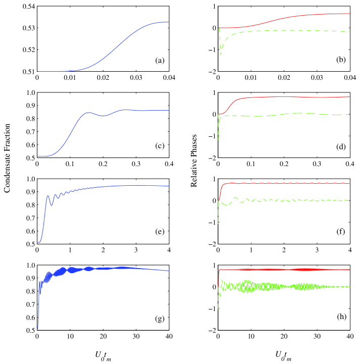
Figure 3: (Color Online) Evolution of the largest condensate fraction and the relative phase parameters for various merging time scales represented by the dimensionless parameter $U_{0}t_{m}$. Figs. (a),(c),(e),(g) are for evolution of the largest condensate fractions, with the merging time scales $U_{0}t_{m}=0.04$, $U_{0}t_{m}=0.4$, $U_{0}t_{m}=4$, $U_{0}t_{m}=40$, respectively. Figures (b),(d),(f),(h) are for evolution of the rotation angle $\theta$ (solid line) and the relative phase $\varphi$ (dashed line), with the merging time scales corresponding to Figs. (a),(c),(e),(g), respectively.

III.3 Merging of two condensates in Fock and coherent states

In this subsection, we investigate the merging of two condensates in a Fock state with $N_{1}=50$ and in a coherent state $\left|\alpha\right\rangle$ with $\left|\alpha\right|^{2}=64$, respectively. This is motivated, on the one hand, by the consideration that the source for an operating atom laser resembles a coherent state; and on the other hand, by the curiosity to find out the influence of the initial number fluctuations on the merging dynamics. A coherent state is certainly not an eigenstate of the Hamiltonian (5) at $t=0$ with $J\left(t\right)\rightarrow 0$, so we start from a superposition of a series of eigenlevels instead of a particular one.

The simulation results are shown in Figs. (4a)-(4e) for the evolutions of the largest condensate fraction $\eta$ and the corresponding parameters ($\theta$, $\varphi$), with the merging time varying from $U_{0}t_{m}=0.04$ to $U_{0}t_{m}=4$. The results are qualitatively similar to the ones displayed in Fig. 3. The main difference is that the final condensate fraction corresponding to the same time scale is notably worse now. This is understandable, as the initial state we start with is not an eigenstate of the governing Hamiltonian and it has significant initial number fluctuation. The coherent state has number fluctuation on the order of $\sqrt{N}$, so from the analysis in Sec. IIC, we expect that the final condensate fraction may reduce by an amount of order $\sqrt{N}/N$, which is pretty close to the results shown in Figs. (4a)-(4e). In our simulation, the coherent state is not large due to the limitation of the computation efficiency; $1/\sqrt{N}$ is therefore not a small factor and we see considerable decrease in the condensate fraction. In more practical cases with $N\sim 10^{6}$, the initial number fluctuation of each condensate should have a much smaller influence on the final condensate fraction.

.

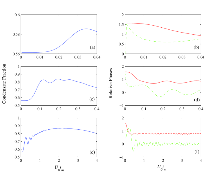
Figure 4: (Color Online) Similar to Fig.3, but with different states for the initial component condensates. One of them is in a Fock state with N=50 and the other is in a coherent state $\left|\alpha\right\rangle$ with $\alpha=8$. The merging time scales are given respectively by $U_{0}t_{m}=0.04$ (Figs. (a),(b)), $U_{0}t_{m}=0.4$ (Figs. (c),(d)), $U_{0}t_{m}=4$ (Figs. (e),(f))

III.4 Comparison of different merging methods

We have mentioned before that the merging dynamics is only determined by the rough time scale in the variations of $U\left(t\right)$ and $J\left(t\right)$, rather than the explicit functional forms of these two parameters. We now verify this result by considering different merging methods. Let us consider two cigar-shaped condensates (with $\sigma_{z}=10\sigma_{\rho}$ in Eq. (7)) merged along the radial and the axial directions, respectively. The variations of $U\left(t\right)$ and $J\left(t\right)$ as functions of time are shown in Fig. (5a) and (5b) for these two cases. For merging along the axial direction, the evolutions of the largest condensate fraction $\eta$ and the corresponding mode parameters ($\theta$,$\varphi$) are shown in Fig. (5c) and (5d) with $U_{0}t_{m}=4$. Compared with the corresponding results for merging along the radial direction, we see there is little difference in the final condensate fraction although the variations of $U\left(t\right)$ and $J\left(t\right)$ differ considerably in the two cases. This shows that what matters most for the merging dynamics is the rough time scale of $U\left(t\right)$ and $J\left(t\right)$ as we have mentioned before. It also justifies our use of the simple Gaussian functions in Eq. (7) to model the individual condensate wave functions, as the functional details of $U\left(t\right)$ and $J\left(t\right)$ are not so important.

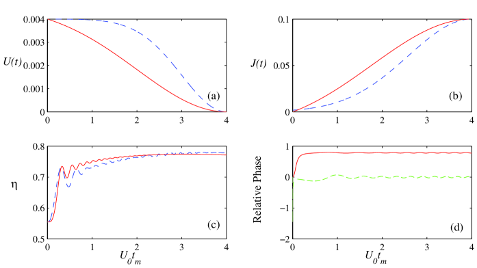
Figure 5: (Color Online) Comparison of the dynamics for merging along different directions. (a)(b) $U$ and $J$ as functions of the dimensionless time while merging along the radial direction (solid line) or the axial direction (dashed line).(c) Comparison of the evolution of the largest condensate fraction $\eta$. The solid line represents merging along the radial direction and the dashed line represents merging along the axial direction. Despite different variations of $U$ and $J$ shown in (a)(b), there seems to be little difference in the evolution of the condensate fraction. (d) Evolution of the rotation angle $\theta$(solid line) and the relative phase $\varphi$(dashed line) when merging along the the axial direction. Qualitatively, it is similar to the evolution shown in Fig. 3(f) for merging along the radial direction.

This result should not be misunderstood as that it is equally good in real experiments to merge the condensates along the radial or the axial direction. Experimentally, for the cigar-shaped condensates, it is much better to merge them along the radial direction 6 . The reason is that we have assumed that the density profile of the atoms can adiabatically follow the movements of the traps to validate the two-mode model. Although that is the case for merging along the radial direction, it will be much harder to meet this condition if the condensates are merged along the axial direction. In the latter case, one needs to have the condensates further away from each other initially to have negligible $J\left(t\right)$ at the beginning; one also needs to move the atoms significantly faster to have the same time scale for merging. However, the trap along the axial direction is much weaker, and a large fraction of the atoms could be excited during the merger. As a result, the atomic density profile would be left behind the movements of the traps unless one reduces the merging speed to an undesirable value (for instance, with a time longer than the condensate life time). Therefore, merging along the weaker trapping direction makes the individual condensate wave functions harder to follow adiabatically the movements of the traps, which would invalidate the two-mode approximation. Nevertheless, if the two-mode approximation could be justified, the relative phase dynamics would then become insensitive to the detailed merging methods, as shown by this numerical simulation.

IV Summary

Using a two-mode model, we have studied the dynamics of relative phase and condensate fraction during the direct merging of two independently prepared condensates with random relative phase. In accordance with a recent experiment6 , we found that it is possible to create a single condensate with larger condensate fraction and a unique zero relative phase between the initial condensate modes. By examining the energy spectrum of the Hamiltonian under the two-mode approximation, the process can be understood both within and without the adiabatic limit. In the ideal adiabatic limit, the result can be explained using the adiabatic theorem, and the system will evolve from a fragmented condensate to a single condensate following the evolution of the eigenstate of the Hamiltonian during the merger. Beyond the adiabatic limit, careful analysis of the evolution of the eigen-spectrum is needed. Qualitatively, due to the quadratic scaling of the excitation energy with the energy levels, only the low-lying eigenstates of the Hamiltonian will be populated even if the process is far from the adiabatic limit. At the end of the merger, the mixture of those low-lying states will give rise to the final state with dominant number of atoms in the desired single condensate mode. Numerical simulations are then performed, and the results are in good agreement with our analysis. The results may have interesting implications for realization of a continuous atom laser based on direct merging of independently prepared condensates. Because of the similarity of our model to the case of condensates in double wells or optical lattice, the adiabatic and non-adiabatic evolution picture described here may also find applications in controlling the dynamics of condensates in those optical potentials.

This work was supported by the ARDA under ARO contracts, the NSF EMT grant, the FOCUS seed funding, and the A. P. Sloan Fellowship.

References

- (1) M. Kozuma et al., Science, 286, 2309 (1999).
- (2) S. Inouye et al., Nature, 402, 641 (1999).
- (3) M.-O. Mewes et al., Phys. Rev. Lett., 78, 582 (1997).
- (4) C.K. Law, N.P. Bigelow, Phys. Rev. A, 58, 4791-4795 (1998).
- (5) M. Holland, K. Burnett, C. Gardiner, J.I. Cirac and P. Zoller, Phys. Rev. A, 54, R1757 (1996).
- (6) R.J.C. Spreeuw, T. Pfau, U. Janicke, and M. Wilkens, Eur. Phys. Lett., 32, 469 (1995).
- (7) H.M. Wiseman, M.J. Collett, Phys. Lett. A, 202, 246 (1995).
- (8) J. Williams, R. Walser, C. Wieman, J. Cooper, and M. Holland, Phys. Rev. A, 57, 2030 (1998).
- (9) B.K. Teo, G. Raithel, Phys. Rev. A,63, 031402 (2001).
- (10) M. Greiner et al., Phys. Rev. A, 63, 031401 (2001).
- (11) D. Jaksch et al., arXiv:cond-mat/0101057 (2001).
- (12) K. Mølmer, Phys. Rev. A, 65, 021607 (2002).
- (13) A.P.Chikkatur et al., Science, 296, 2193 (2002).
- (14) I. Zapata, F. Sols, and A.J. Leggett, Phys. Rev. A, 67, 021603 (2003).
- (15) J. Javanainen, M.Y. Ivanov, Phys. Rev. A, 60, 2351 (1999).
- (16) K.W. Mahmud, H. Perry, and W.P. Reinhardt, arXiv:cond-mat/0312016 (2003).
- (17) R.W. Spekkens, J.E. Sipe, Phys. Rev. A, 59, 3868 (1999).
- (18) G.J. Milburn, J. Corney, E.M. Wright, D.F. Walls, Phys. Rev. A, 55, 4318, (1997).
- (19) C. Menotti, J.R. Anglin, J.I. Cirac and P. Zoller, arXiv:cond-mat/0005302 (2000).
- (20) A.J. Leggett, Rev. Mod. Phys., 73, 307 (2001).
- (21) D. Wagner, J. Phys. A: Math. Gen., 15, 3307 (1982).
- (22) We have assumed that the two traps are initially symmetric. In this case, the system is in a low-energy state only when . It is possible to generalize the results to the case where the initial two traps are asymmetric and for the low energy state.
- (23) V.K. Thankappan, Quantum Mechanics (Pergamon Press, New York 1993).
- (24) It is very hard to control the initial atom number of each condensate to be exactly the same (). We assume there is a number flucation on the order of around this mean value, corresponding to the so-called shot-noise limit.
- (25) M. Holthaus, S. Stenholm, Eur. Phys. J. B, 20, 451 (2000).
- (26) G-S. Paraoanu et al., J. Phys. B: At. Mol. Phys., 34, 4689 (2001).