Phase-Modulus Relations for a Reflected Particle

Abstract

We formulate analytically the reflection of a one dimensional, expanding free wave-packet (wp) from an infinite barrier. Three types of wp’s are considered, representing an electron, a molecule and a classical object. We derive a threshold criterion for the values of the dynamic parameters so that reciprocal (Kramers-Kronig) relations hold in the time domain between the log-modulus of the wp and the (analytic part of its) phase acquired during the reflection. For an electron, in a typical case, the relations are shown to be satisfied. For a molecule the modulus-phase relations take a more complicated form, including the so called Blaschke term. For a classical particle characterized by a large mean momentum ($\hbar K>>\frac{\hbar~{}trajectory~{}length}{(size~{}of~{}wave-packet)^{2}}>>>\frac{\hbar}{size~{}of~{}wave-packet}$) the rate of acquisition of the relative phase between different wp components is enormous (for a bullet it is typically $10^{14}$ GHertz) with also a very large value for the phase maximum.

1 Background and Introduction

Textbooks of quantum mechanics contain accounts of the impingement of a freely moving one-dimensional particle on a finite- or an infinite-height barrier (e.g., ref. 1) Some further developments in ref. 2 and more recently in ref. 3 derived the intensity or modulus of the particle beyond a barrier. In some of these works the particle is modelled by a incoming plane wave with a given momentum. Other related works are ref. 4 and, on the experimental side, ref. 5. In so much as at some later stage in this study we obtain the location of the zeros of the reflected wave, we note the recent interest in the distributions of zeros (nodes) of a (chaotic) wave ^6,7 in the coordinate space.

Using an elementary and exactly soluble model, we consider here a localized wave packet (wp) representing, for instance, a microscopic particle, such as an electron and a molecule, reflected from an infinitely high barrier. One of our purposes is to investigate the phase of the wp during its history and to unravel a possible relation between the phase and the modulus of the wp. Such relations were treated in our earlier articles $~{}^{8-10}$, and this work can be considered an extension.

We further consider the wp of a classical particle and look at its phase behavior. The interest in this lies in the widely held belief that in any quantum mechanical measuring-process the phase interference between the measured quantum system and its classical enclosure plays a crucial role (e.g., ref. 11 ). An opposite view has been recently expressed in ref. 12.

2 Description of the Model

The particle is represented as a one-dimensional expanding wave-packet (wp), starting at time $t=0$ as a Gaussian form centered at a point $x=a$ and having initially a width $2\Delta$, that is as

$$\psi(x,a,t)=\frac{1}{\sqrt{\Delta}}\exp\big{[}-\frac{(x-a)^{2}}{4\Delta^{2}}\big{]}\exp\big{[}iK(x-a)]$$ (1)

$K$ is defined in terms of the mean particle momentum $p$ by $K=\frac{p}{\hbar}$ and the crossed Planck constant $\hbar$. The particle (whose physical mass is $m_{physical}$) moves to the right, until it impinges on an infinite barrier at $x=0$ (so that $a$ is negative). It is then, reflected from the barrier and moves left-wards, as depicted in figure 1.

\begin{picture}(1.0,1.0)\end{picture}

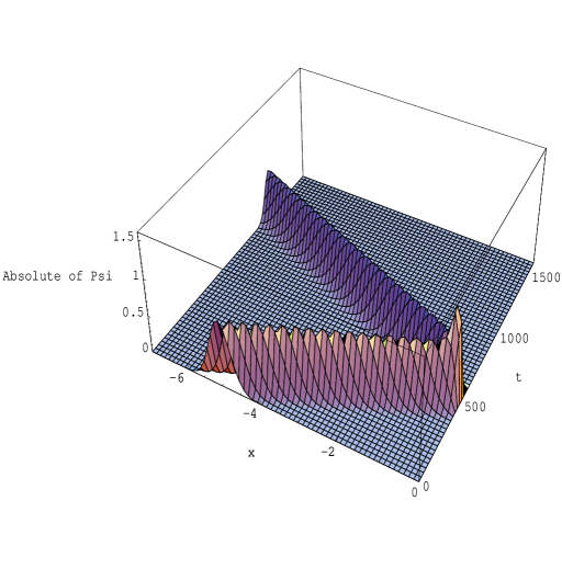
Figure 1: Time-motion plot of the wave-packet of a particle reflected by a boundary placed at $x=0$. The particle starts at $x=-5$. (The units employed vary with the nature of the particle: an electron, a molecule or a macroscopic projectile.)

Following Tomonaga ¹³ and other elementary texts, we write the wave-function $\psi$ of a freely moving wp (without a barrier) and satisfying a time dependent Schrödinger equation, as

$$\psi(x,a,t) = \frac{1}{\sqrt{(}\Delta+\frac{it}{2m\Delta})}exp\big{[}-\frac{(x-a)^{2}-4i\Delta^{2}K(x-a-\frac{Kt}{2m})}{4\Delta^{2}+\frac{2it}{m}}\big{]}$$ (3)

$$= (\frac{1}{\Delta^{2}+\frac{t^{2}}{4\Delta^{2}m^{2}}})^{\frac{1}{4}}\exp\big{[}-\frac{(x-a-\frac{Kt}{m})^{2}}{4\Delta^{2}+\frac{t^{2}}{\Delta^{2}m^{2}}}\big{]}\exp\big{(}-\frac{i}{2}arctan\frac{t}{2\Delta^{2}m}\big{)}$$

$$\exp\big{[}i\frac{K(x-a-\frac{Kt}{2m})+\frac{(x-a)^{2}}{8\Delta^{2}}\frac{t}{m\Delta^{2}}}{1+\frac{t^{2}}{4\Delta^{4}m^{2}}}\big{]}$$

The symbol $m$ is related to the physical mass by $m=\frac{m_{physical}}{\hbar}$. In the second expression the wave function appears as a product of the (real) modulus and a pure phase factor. The group (or amplitude) velocity is $\frac{Kt}{m}$, the same as the velocity of a classical particle, but the phase velocity is seen to be more complicated. It is noted for future reference that when the above free wp is considered as a function of the complex time

$$t=t^{\prime}+it"$$ (4)

it is regular function in the lower half of the complex $t$-plane ($t"<0$) and tends to zero for large $|t|$. The former property is shared by all physical wave-packets in a time-independent environment, and is due to the lower boundedness of the energy (or frequency) spectrum (which implies that wave functions of a freely moving particles with negative energies are all zero ^14,10. This property is analogous to the principle of causality, which makes the response functions to be zero at negative times and by consequence, ensures the analyticity of response functions in the upper half of the complex frequency plane ¹⁵.

It will be noticed that the wp has a branch point and an essential singularity in the upper half of the $t$- plane.

In the presence of an infinite barrier the wave function, to be written as $\Psi(x,t)$, has to satisfy the condition

$$\Psi(x,t)=0~{}~{}\ for~{}x=0$$ (5)

at all times and to vanish at $x=-\infty$ at finite times. A suitable solution is thus

$$\Psi(x,t)=N[\psi(x,a,t)-\psi(-x,a,t)]~{}~{}for~{}x<0$$ (6)

and

$$\Psi(x,t)=0~{}~{}for~{}x\geq 0$$ (7)

The real, positive quantity $N$ in equation (6) is a normalizing factor, given by

$$N^{-2}=\int_{-\infty}^{0}dx{|\Psi(x,t)|^{2}}$$ (8)

and is independent of time. This result follows from the integration of the continuity (or mass-conservation) equation, account being taken of the vanishing of the integrand at $x=-\infty$ and at $x=0$.

3 The convergent difference function

The full wave function $\Psi(x,t)$ shown in equation (6) can be expressed as a product of the incoming wave function ($\psi(x,t)$ shown in equation (3) ) and the ”difference function” $\chi^{\prime}(x,t)$ defined as

$$\chi^{\prime}(x,t)=1-\frac{\psi(-x,t)}{\psi(x,t)}$$ (9)

From equation (3) this is

$$\chi^{\prime}(x,t)=1-e^{\frac{-4x(2iK\Delta^{2}+a)}{4\Delta^{2}+\frac{2it}{m}}}$$ (10)

This function contains the effect of the reflection on both the amplitude and the phase of the total wave function. We now introduce a new function $\chi(x,t)$ , given by

$$\chi(x,t)=\frac{4\Delta^{2}+\frac{2it}{m}}{4x(2iK\Delta^{2}+a)}(1-e^{\frac{-4x(2iK\Delta^{2}+a)}{4\Delta^{2}+\frac{2it}{m}}})$$ (11)

differing from the (former) difference function $\chi^{\prime}(x,t)$ only by the fraction shown. This function has the desired analytical property of tending to 1 as $|t|\to\infty$. By consequence $\ln\chi(x,t)\to 0$ and we shall be able to use this function in an integration of the logarithm over $t$ with infinite limits in the formulae that follow. $\chi(x,t)$ is thus termed the ”convergent difference function” and has (in certain physical situations, to be specified later) the properties postulated in ref. 8-10 for Hilbert transforms.

3.0.1 Reciprocal relations

The validity of the following formulae requires $\ln\chi(x,t)$ to be analytic in the lower half of the complex t-plane and to tend to zero as $|t|\to\infty$.

$$\frac{1}{\pi}P\int_{-\infty}^{\infty}dt^{\prime}[\ln|\chi(t^{\prime})|]/(t-t^{\prime})=-\arg\chi(t)$$ (12)

and

$$\frac{1}{\pi}P\int_{-\infty}^{\infty}dt^{\prime}[\arg\chi(t^{\prime})]/(t-t^{\prime})=\ln|\chi(t)|$$ (13)

Here P signifies the principal part of the singular integral. (For a derivation and extensions of these formulae when not all the conditions are met, see ref. 16 or 9.)

3.1 Zeros of the difference function

Evidently $\chi(x,t)$ has no singularities in the lower half of the complex $t$-plane. However, since our interest is in the logarithm, we need to examine not only the singularities but also the zeros of $\chi(x,t)$. These will come about when the exponent in equation (6) is zero or an integer times $2\pi$. Writing in the sequel $-|x|$ for $x$ and $-|a|$ for $a$ (since both quantities are negative) and equating

$$\frac{4|x|(2iK\Delta^{2}-|a|)}{4\Delta^{2}+\frac{2it}{m}}=2i\pi n$$ (14)

(where $n$ is a positive or a negative integer or zero), we find the location of the $n$’th zero in the complex $t$-plane ($t=t^{\prime}+it"$), at any fixed location $-|x|$ on the left of the barrier as follows:

$$t_{n} = t^{\prime}_{n}+it"_{n}$$ (15)

$$t^{\prime}_{n} = m\frac{|x||a|}{n\pi},~{}~{}~{}t"_{n}=2\Delta^{2}m(1-\frac{K|x|}{n\pi})$$ (16)

The time when the center of the wave is reflected from the barrier is denoted by $t_{r}$ and is

$$t_{r}=\frac{m|a|}{K}$$ (17)

whereas the time (to be denoted by $t_{d}$) when the wp broadens due to its intrinsic dynamics in excess of its original width is given by

$$t_{d}=2m\Delta^{2}$$ (18)

We next define for any fixed point $x$ to the left of the barrier the dimensionless quantity $n_{r}(x)$ given by

$$n_{r}(x)=\frac{|x|K}{\pi}$$ (19)

In terms of the quantities defined, the location of the zeros in the $t$-plane can be written as

$$t^{\prime}_{n}=t_{r}\frac{n_{r}(x)}{n},~{}~{}t"_{n}=t_{d}(1-\frac{n_{r}(x)}{n})$$ (20)

Note that we shall always have zeros on the upper half of the complex $t$-plane, since $n$ can be a negative integer, but zeros on the lower half of the complex plane can exist only for $n$ a positive integer which satisfies

$$n_{r}(x)>n$$ (21)

This implies that when

$$n_{r}(x)~{}<~{}1$$ (22)

there are no zeros on the lower half of the complex plane (since equation (21) cannot be satisfied for any positive integer). Therefore, the reciprocal relations in equation (12) and equation (13) can be applied to obtain the additional reflection-induced phase through the change in amplitude of the wave. Thus under this condition the reflection-induced phase is an observable quantity.

The above inequality amounts to the following:

$$|x|p~{}<~{}\pi\hbar$$ (23)

The above two inequalities are among the central results of this work and are termed ”Analyticity thresholds for a reflected particle”. They can be achieved if the distance of observation $|x|$ from the position of the barrier is short, or if the mean momentum $p$ of the particle is small. The latter condition can be achieved, as we shall see, for a particle with a microscopic mass or for an extremely slowly moving projectile. The momentum-position uncertainty relations are not violated by equation (23) , since $p$ is not the measured momentum of the particle, only a parameter in the preparation of the projectile. Likewise, $x$ is a parameter of the measurement, whose outcome is a spread-out function (the wp modulus).

In terms of the parameters introduced in this section, the difference function can be written more simply as

$$\chi^{\prime}(t)~{}=~{}1-\exp\big{[}i\pi n_{r}(x)\frac{t_{r}-it_{d}}{t-it_{d}}\big{]}$$ (24)

4 Applications

We consider three cases for which the wavepacket in equation (6) can serve as prescriptions.

4.1 An electron

The wp of this can be characterized by the following parameters (all in atomic units): $m=1(=m_{e}$, electronic mass), $a=-5$, $v$ (velocity)$=K/m=2$, $\Delta=2$, $x=-1.5$

Then $|x||K|=3$, $E=2$, $t_{r}=\frac{m|a|}{K}=2.5$, $\pi n_{r}(x)=|x||K|=3$, $t_{d}=8$,

$$t^{\prime}_{n}=\frac{7.5}{\pi n},~{}~{}~{}t"_{n}=8(1-\frac{3}{\pi n})$$ (25)

where n is zero or a positive or negative integer. It then follows that $t"_{n}<0$ for all $n$. Thus, all zeros of the difference function $\chi(t)$ lie in the upper half of the $t$-plane. By consequence $\ln\chi(t)$ is analytic in the lower half-plane and vanishes on a large semi-circle there. This ensures the validity of the reciprocal relations shown in equation (12) and equation (13) .

We illustrate the use of the reciprocal relations in Figure 2.

\begin{picture}(1.0,1.0)\end{picture}

Figure 2: The ”analytical phase”. This is the part of the phase coming from the analytic difference function $\chi(x,t)$ (here plotted for an electron against time $t$ in the vicinity of the reflection time $t_{r}$ and for $x=-1.5$, all in atomic units). The phase shown by full lines is calculated from the log-modulus, using one of the two conjugate reciprocal relations. The curve drawn by broken lines is calculated directly as the argument of the complex function of $\chi(x,t)$. It shows jumps of $\pm 2\pi$.

The curve shown by full lines is obtained by calculating the argument indirectly, from the modulus through equation (12) . The broken line curve, shown for comparison and displaced by a tiny amount for clarity, is computed directly from the expression in equation (11) . It is clear that the two curves represent the same quantity calculated in two different ways.

Apart from verifying the analytical properties of $\chi(x,t)$, the agreement between the curves in Figure 2 provides a further instance for the possibility, achievable under suitable circumstances, that for a wp the analytic part of the phase is precisely given by the values of the wave-function modulus for real values of the time. (The ”analytic” part is obtained from the total, physical phase by subtracting from the latter those quantities that do not vanish at $t=\pm\infty$.) This part of the phase is ”observable”, indirectly, through the modulus.

The value of $x$ chosen for this case, namely .08 nanometers, is near the analyticity threshold value for the chosen mean particle momentum.

4.2 A molecule

As the next example (and still staying inside the microscopic domain) we take an impacting water molecule (molecular weight: 18) with the following kinetic parameters expressed in atomic units: $m=3.6~{}10^{4}$, $a=-10$, $v$ (velocity)$=K/m=2.8~{}10^{-4}$, $K=10$, $x=-4$. For the wave packet width we use a value taken from ref. 18, namely $\Delta=.3$ (also in atomic units). This is of the order of the zero point motion amplitude of the nuclei. The coordinate $x$ represents the position of the center of mass of the molecule, with other internal degrees of freedom considered fixed during the motion.

We further take $|x||K|=40$, $E=1.4~{}10^{-3}$, $t_{r}=\frac{m|a|}{K}=3.6~{}10^{4}$, $\pi n_{r}(x)=|x||K|=40$, $t_{d}=3.1~{}10^{3}$,

$$t^{\prime}_{n}=\frac{1.4~{}10^{6}}{\pi n},~{}~{}~{}t"_{n}=3.1~{}10^{3}(1-\frac{40}{\pi n})$$ (26)

The zeros of the difference function are shown in Fig. 3.

\begin{picture}(1.0,1.0)\end{picture}

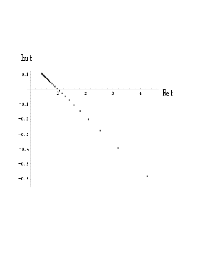
Figure 3: Argand plot in the complex $t(=t^{\prime}+it")$ plane for the location of zeros in the difference function for a reflected water molecule. The physical parameters are as given in the text for a molecule. For these there are an infinite number of zeros in the upper-half and 12 zeros in the lower-half of the complex t-plane. We show about 30 zeros lying nearest to the real axis. The zeros are plotted in units of the reflection time $t_{r}$, defined in the text and (with the present choice of parameters) having a value of $3.6~{}10^{4}$ in atomic units.

for values of $n$ in the neighborhood of the sign change in the imaginary part $t"_{n}$, namely near $n=13\approx 40/\pi$.

The position- threshold for analyticity in the case of a molecule that has the quoted dynamic parameters is .02 nanometer, which is hardly accessible to measurements. Thus for a molecule the determination of phase from modulus values requires the consideration of the Blaschke term, as noted in $~{}{16}$.

4.3 A classical object

We express the parameters of the wp, now in mgs units, as follows: $m=1$, $v=100$, $mv=\hbar K=10^{2}$, ($\hbar\approx 10^{-31}$), $K=10^{33}$, $|x|=0.1$, $E=.5~{}10^{2}$ and in terms of an angular frequency, (in inverse second units) = $E/\hbar=.5~{}10^{33}$, $t_{r}=10^{-2}$, $\pi n_{r}(x)=|x||K|=10^{32}$, $t_{d}=2~{}10^{9}$.

The choice of the initial wp width $\Delta$ requires some thought, since it is not a usual quantity for a classical object. A lower limit is clearly the zero point motion amplitude for a single vibrational mode in the object. This is similar to that used for a molecule, above, and amounts to $\Delta=10^{-11}$, in the now used mgs units. It could be argued that the large number of vibrational modes in the solid (of the order of $10^{8}$ modes in the direction of motion), would demand a larger number, e.g. through multiplication of the previous conjecture by the square root of the number of modes, leading to $\Delta=10^{-7}$. We shall see, however, that this latter number does not change qualitatively the essential conclusions reached in this section, namely, that at about the instant of the reflection, the wp acquires a very large phase shift, due to the difference function.

Thus, with the former, smaller choice for $\Delta$,

$$t^{\prime}_{n}=\frac{10^{30}}{\pi n},~{}~{}~{}t"_{n}=2~{}10^{9}(1-\frac{10^{32}}{\pi n})$$ (27)

Because of the very large numbers involved, the discussion that follows will be in terms of orders of magnitudes.

4.3.1 The reflectional phase shift

We first rewrite the difference function in equation (24) as

$$\chi^{\prime}(t)~{}=~{}1-e^{\big{[}i\pi n_{r}(x)\frac{1+\frac{it_{r}}{t_{d}}}{1+\frac{it}{t_{d}}}\big{]}}$$ (28)

so that the time-quotients in the exponents are small and whose powers beyond the first can be ignored. We first compute the phase-change (arising from the difference function only) acquired during the full motion. Initially at $t=0$ we compute (using the linear approximation in small quantities)

$$\chi^{\prime}(0)~{}=~{}1-e^{-i\pi n_{r}(x)}e^{-\pi\frac{n_{r}(x)t_{r}}{t_{d}}}=1-e^{-i\pi n_{r}(x)}\exp\big{[}-\frac{1}{2}10^{32-2-9}\big{]}\approx 1$$ (29)

Thus, the phase is zero initially. Long after the reflection, but before disintegration of the wp $(t_{d}>t>>t_{r})$

$$\chi^{\prime}(0) = 1-e^{i\pi n_{r}(x)}e^{\pi\frac{n_{r}(x)t}{t_{d}}}\approx 1-e^{i\pi n_{r}(x)}\exp[10^{30}]\$$ (30)

$$\approx e^{i\pi n_{r}(x)}\exp[10^{30}]\$$

The phase acquired is thus approximately $\pi n_{r}(x)=|x|K\approx 10^{32}$. What is essential to note is that this phase scales with the momentum of the classical particle $K$.

4.3.2 The phase at reflection

Let us next consider the phase change at about the reflection time $t_{r}$ (measured at a point positioned at $|x|=0.1$ meter before the barrier). To this end we expand the exponent for $t\approx t_{r}$ and obtain

$$\chi^{\prime}(0)~{}=~{}1-e^{i\pi n_{r}(x)}e^{\pi n_{r}(x)\frac{t-t_{r}}{t_{d}}}\approx 1-e^{i\pi n_{r}(x)}\exp[\frac{1}{2}~{}10^{21}(t-t_{r})]$$ (31)

It is clear that the amplitude of the second (complex) term changes around $t=t_{r}$ from a very small number to a very large one. The rate of change is easily calculated to be

$$\frac{|x|K\hbar}{\frac{1}{2}m\Delta^{2}}=\frac{|x|v(the~{}velocity)}{\frac{1}{2}\Delta^{2}}=2~{}10^{23}(radians~{}per~{}second)$$ (32)

It should be noted that the astronomical large value of this rate will still remain large $(\approx 10^{15})$ when the initial value of the wp width is increased $10^{4}$-fold.

On the other hand, the rate of phase-change of a freely evolving classical wave packet (in the absence of barrier) will be larger $(\approx 10^{44})$ by many orders of $10$. This change remains also for the reflected particle, having regard to the factorization of $\Psi$ as described at the beginning of section 3. The pigmied reflection-induced phase may thus be thought to be devoid of any physical significance. However, the former phase is the total phase of the wp and is not in general observable, whereas the reflection-induced phase is the relative phase between components of the wp, which can be measured by interferometric methods.

While it may be said that the extremely large numbers met with in this section for a macroscopic particle give the results a surrealistic look, one notes that similar extremely high rates ($10^{19}s^{-1}$) are at the base of some proposals for wave function collapse as being due to phase-decoherence $~{}^{19,20}$. We further discuss this connection in the concluding section.

The analyticity threshold for the position of the observation has, for a macroscopic projectile, an extremely low, sub-nucleonic value and is not realistic.

5 Conclusion

We have presented an analytic formulation for an elementary one- dimensional scattering process of a microscopic wave-packet, perhaps the most elementary one for which an exact, analytic solution is available. It has been shown that under circumstances that are realizable for an electron, reciprocal relations hold between the phase and the modulus of the scattered particle’s wave function. This supplements our previous demonstrations of the existence of reciprocal relations for localized, bound states $~{}^{8-10}$. In those publications we have noted some other relations that connect the phase with modulus, in particular, the equation of continuity. However, this equation is a partial differential equation and does not uniquely reconstruct the phase, even when the modulus is completely given. Thus, even for a problem in only one spatial dimension, the addition to the position-derivative of the phase of a quantity $\phi(t)/|\psi(x,t)|^{2}$, where $\phi(t)$ is arbitrary, will satisfy the continuity equation, while in higher dimensions a much larger family of functions will do so. In contrast, the reciprocal relations give the analytic part uniquely from the modulus.

The physical basis for these relations was elucidated in $~{}^{14,15}$ , as being due to the lower-boundedness of the energies. When the analyticity requirements are not fully satisfied, e.g., through there being nodal points in the wave function, the phase is still obtainable from the modulus, the latter being given as function of the complex time. When the analytic properties postulated in this article hold fully, it is sufficient to know the modulus as function of real time, i.e., along the real t-axis.

In this paper we have obtained threshold relations which delimit the straightforward application of the reciprocal relations. It will be of interest to extend the theory to three dimensional scattering problems, to finite-height barriers and to other cases.

For a (rigid) molecule impinging on an infinite barrier, we have found that one should expect zeros of the ”difference function” in the lower-half of the complex time-plane, such that additional (so called, Blaschke) terms are required to correlate the modulus with the phase changes.

When the barrier is not infinite, the algebraic, image wave-function solution used in this work is not applicable. For that situation we have developed a method that employs a transfer matrix for each momentum state and we are in the process of obtaining results from this method.

In a further application of the formalism, the reflection of a classical particle from an infinite barrier is characterized by an extremely rapid rate of growth of the wave-function phase and by its attaining a very high value. Having taken for the particle’s mass 1g and for its velocity 100 m/s, we obtain for the rate of phase change at reflection, values of the order of $10^{23}$ radians per second. The precise values, coming from the difference function in equation (11) , depend on the distance from the barrier and from the starting point of the particle.

The acquisition by classical systems of very large phases within a very short time period is likely to be quite general. It is expected that it is rooted in the reciprocal relations between the two quantities (moduli and phases) or, equivalently, in the circumstance that they are parts of the same analytic function. Thus as the $logarithm$ of the modulus increases (numerically), then so does the phase.

While it is of a speculative nature, one would imagine a similar phenomenon to occur during a wave-function collapse. It is widely held that the collapse is caused by a (phase-) decoherence process, which takes place while the quantum component is coupled to (entangled with) the classical component (e.g. ref. 11). On the basis of our results that the sudden switching from one (positive mean momentum) state to another (negative mean momentum) state by a macroscopic object causes the sudden acquisition of a large phase, we might expect a similar phase-increase to occur in the macroscopic part of the combined quantum-classical system. A tiny variation in this macro-phase will suffice to cause decoherence in the total wave -function. However, a detailed description of this process requires further work, probably through use of one the proposed models for decoherence $~{}^{11}$.

6 References

(1) Messiah, A. Quantum Mechanics Vol II North Holland, Amsterdam 1961) Chapter XVII.

(2) R. Winter, R. Phys. Rev. 1961, 123, 1503.

(3) Dicus,D.A.; Repko, W.A.; Schwitters, R.F.; T.M. Tinsley, T.M. Phys. Rev. A 202, 65, 032116.

(4) Kalbermann, G. J. Phys. A: Math. Gen. 2001, 34, 36465; quant-phys/02030036 (5 July 2002).

(5) Savalli, V.; Stevens, D.; Esteve, J.; Featonby, P.D.; Josse, V.; Westbrook, N.; Westbrook C.I.; Aspect, A. Phys. Rev. Lett. 2002 88, 250404.

(6) Berry, M.V.; J. Phys. A: Math. Gen. 2002, 35, 3025.

(7) Bies, W.E.; Heller, E.J.; J. Phys. A: Math. Gen. 2002, 35, 5673.

(8) Englman, R.; Yahalom, A.; Baer, M. Phys. Lett. A 1999, 251, 223.

(9) Englman, R.;Yahalom, A.; Phys. Rev. A 1999, 60, 1802.

(10) Englman, R.; Yahalom, A. A͡dv. Chem. Phys. 2002, 124, 197.

(11) Omnes, R.; Phys. Rev. A 2002, 65, 052119.

(12) Adler, S.; J. Phys. A: Math. Gen. 2002, 35, 841.

(13) Tomonaga, S.-I. Quantum Mechanics Vol. II (North Holland, Amsterdam, 1966 Sections 41 and 61.

(14) Khalfin, L.A. Soviet Phys. JETP 1958, 8, 1053.

(15) Perel’man, M.E.; Englman, R. Modern Phys. Lett. 2001, 14, 907.

(16) Toll, J.S.; Phys. Rev. 1956, 104, 1760.

(17) Gogtas, F.; Balint-Kurti, G.G.; Offer, A.R. J. Chem. Phys. 1996, 104, 7927.

(18) Ghirardi, G.; Rimini, A.; Weber, T. Phys. Rev. D, 1986, 34, 470.

(19) Pearle, P.; Squires, E. Phys. Rev. Lett. 1994, 73 1.