Giant Lamb shift in photonic crystals

Abstract

We obtain a general result for the Lamb shift of excited states of multi-level atoms in inhomogeneous electromagnetic structures and apply it to study atomic hydrogen in inverse-opal photonic crystals. We find that the photonic-crystal environment can lead to very large values of the Lamb shift, as compared to the case of vacuum. We also predict that the position-dependent Lamb shift should extend from a single level to a mini-band for an assemble of atoms with random distribution in space, similar to the velocity-dependent Doppler effect in atomic/molecular gases.

Since the pioneering experiment performed by Lamb and Retherford Lamb in 1947 and the subsequent theoretical analysis developed by Bethe Bethe , the study of the Lamb shift plays an unique role in quantum electrodynamics (QED) because it provides an excellent test of the QED theory by comparing its predictions with experimental observations van ; Karsh . Recently, many efforts have been devoted to the study of various physical effects associated with the Lamb shift Vlad ; Yu ; Chai .

Photonic crystals (PCs) are a new type of optical material with a periodic dielectric structure s_john . They can pronouncedly modify the photonic density of state (DOS) and local DOS leading to novel quantum-optics phenomena sakoda such as inhibition ES and coherent control Quang of spontaneous emission, enhanced quantum interference effects Zhu1 , non–Markovian effects Bay ; John1 , wide lifetime distribution wangxh1 , non-classic decay wangxh2 , and slop discontinuities in the power spectra alva , etc.

Strong suppression or enhancement of light emission by the PC environment is expected to modify the Lamb shift. However, very different predictions for the Lamb shift can be found in literature. The isotropic dispersion model John2 predicts an anomalous Lamb shift and level splitting for multi-level atoms. For two-level atoms, the anisotropic model Zhu2 suggests that the Lamb shift should be much smaller than that in vacuum, while the pseudogap model Vats predicts a change of the Lamb shift of the order of $15\%$ compared to its vacuum value. At last, a direct extension of the Lamb shift formulism for multi-level atoms in vacuum to the case of PCs suggests that the Lamb shift differs negligibly from its vacuum value Li .

Motivated by previous controversial results, in this Letter we employ the Green’s function formalism of the evolution operator to obtain a general result for the Lamb shift in PCs. We reveal that in an inhomogeneous electromagnetic environment the dominant contribution to the Lamb shift comes from emission of real photon, while the contribution from emission and reabsorption of virtual photon is negligible, in vast contrast with the case of free space where the virtual photon processes play a key role. The properties of the Lamb shift near the band gap are calculated numerically for an inverse opal PC. We find that the PC structure can lead to a giant Lamb shift, and the Lamb shift is sensitive to both the position of an atom in PCs and the transition frequency of the related excited level.

We study the Lamb shift in PCs in the framework of nonrelativistic quantum theory. For an multi-level atom located at the position ${\bf r}$ in a perfect 3D PC without defects, Hamiltonian of the system can be presented in the form $H=H_{0}+H_{\rm int}+H_{\rm ct}$, where the term $H_{0}$ stands for noninteracting Hamiltonian and the term $H_{\rm int}$ describes interaction between an atom and photons, so that

$$H_{0}+H_{int}=\frac{{\bf p}^{2}}{2m}+V_{a}+\hbar\sum_{n\bf{k}}\omega_{n\bf{k}}a_{n\bf{k}}^{+}a_{n\bf{k}}+\frac{e}{m}{\bf p}\cdot{{\bf A}({\bf r})}$$ (1)

with ${\bf A}({\bf r})=\sum_{n\bf{k}}(\hbar/2\varepsilon_{0}\omega_{n\bf{k}})^{1/2}[{\bf E}_{n}({\bf k},{\bf r})a_{n{\bf k}}+\mbox{H. C.}]$ being the quantized vector potential, the second-order term of the vector potential in Eq. (1) has been neglected, and $H_{\rm ct}=(\delta m/m){\bf p}^{2}/2m$ is a mass-renormalization counter-term for an electron of observable mass $m$ John2 ; Loui . The electromagnetic (EM) eigenmodes $\{\omega_{n{\bf k}},{\bf E}_{n{\bf k}}({\bf r})\}$ in PCs can be found by the plane-wave expansion method Ho .

We assume that an atom is excited initially, and it stays at the $l$-th energy level without a photon in the EM field, and denote $\mid I>=\mid l,0>$ and $\mid F^{j}_{nk}>=\mid j,1_{n{\bf k}}>$ (i.e. the atom is at the level $j$ and the EM field has a photon in the state $n{\bf k}$) as the initial and final states of the system, respectively. The state vector of the system evolves according to the equation, $\mid\Psi(t)>\equiv U(t)\mid I>=C_{i}(t)\mid I>+\sum_{j,n{\bf k}}C^{j}_{n{\bf k}}(t)\mid F^{j}_{nk}>$, with the initial conditions $C_{i}(0)=1$ and $C_{n{\bf k}}(0)=0$, where $U(t)$ is the evolution operator. Applying the Green’s function technique to the evolution operator, we obtain the Fourier transform $C_{i}(\omega)$ of $C_{i}(t)$ in the form cohen ,

$$C_{i}(\omega)=\frac{1}{2\pi i}\left[G_{ii}^{-}(\omega)-G_{ii}^{+}(\omega)\right]~{},$$ (2)

with $G_{ii}^{\pm}(\omega)=\lim_{\eta\rightarrow 0_{+}}<I\mid G(z=\omega\pm i\eta)\mid I>,$ where $G(z)$ is defined by the operator identity $G(z)(z-H/\hbar)=1$. Projecting this operator identity onto the one-photon Hilbert space lamb and noting that the nonvanishing matrix elements of $H_{\rm int}$ are $<F^{j}_{n{\bf k}}\mid H_{int}\mid I>$, we obtain the following analytic expression

$$G^{\pm}_{ii}(\omega)=\lim_{\eta\rightarrow 0^{+}}\frac{1}{(\omega-\omega_{l})-\Delta\pm i[\Gamma/2+\eta]},$$ (3)

where $\Gamma=\sum_{j}\alpha_{lj}g({\bf r},\omega-\omega_{j})$, $\Delta=\sum_{j}(\alpha_{lj}/2\pi)(\omega-\omega_{j})\beta({\bf r},\omega-\omega_{j})$, and

$$g({\bf r},\omega)=\displaystyle{\frac{c^{3}V_{pc}}{8\pi\omega}\sum_{n}\int_{BZ}d{\bf k}\mid{\bf E}_{n\bf k}({\bf r})\mid^{2}\delta(\omega-\omega_{n{\bf k}})},$$ (4)

$$\beta({\bf r},\omega-\omega_{j})={\cal P}{\displaystyle\int^{\omega_{\rm rel}}_{0}\frac{g({\bf r},\omega^{\prime})}{(\omega-\omega_{j}-\omega^{\prime})\omega^{\prime}}d\omega^{\prime}}.$$ (5)

Here $V_{pc}$ is the PC volume, $\omega_{\rm rel}=mc^{2}/\hbar$ is the relativistic limit of the photon energy Bethe , $\alpha_{lj}=e^{2}|{\bf p}_{lj}|^{2}/3\pi m^{2}\epsilon_{0}\hbar c^{3}$ is the relative line width of the atomic radiation from the $l$-state to $j$-state in vacuum, and $\cal P$ stands for the principal value of the integral. In Eqs. (4) and (5), we have considered a random orientation of ${\bf p}_{lj}$ and include the mass-renormalization contribution, respectively Loui ; John2 ; Zhu2 ; Vats ; Li . The function $g({\bf r},\omega)$ is the local spectral response function (LSRF) proportional to the photon local DOS.

Equations (2) and (3) show that the radiative correction to the bound level $l$ is determined by the expression

$$(\omega-\omega_{l})=\sum_{j}\frac{\alpha_{lj}}{2\pi}(\omega-\omega_{j})\beta({\bf r},\omega-\omega_{j}).$$ (6)

In the two dispersion models, $|{\bf E}_{n{\bf k}}({\bf r})|^{2}=1/V_{pc}$(V²/m²), then Eq. (6) just gives the results described by Eq. (6a) of Ref. John2 provided we take $l=1$. For a two-level atom with $j=0,1$, we note that $\alpha_{11}=0$ due to ${\bf p}_{11}\equiv 0$ (${\bf p}_{lj}=i(\omega_{l}-\omega_{j})m{\bf r}_{lj}$), and Eq. (6) can be simplified to Eq. (4.9) of Ref. Vats by setting $l=1$ and $\omega_{0}$ as zero point of energy. In vacuum, $g({\bf r},\omega^{\prime})=\omega^{\prime}$, and by setting $\omega=\omega_{l}$ in the right-hand side of Eq. (6), we obtain

$$\Delta^{0}_{l}=\frac{e^{2}}{6\pi^{2}m^{2}\epsilon_{0}\hbar c^{3}}\sum_{j}-\omega_{jl}|{\bf p}_{lj}|^{2}\beta({\bf r},-\omega_{jl}),$$ (7)

where $\omega_{jl}=\omega_{j}-\omega_{l}$ and $\beta({\bf r},-\omega_{jl})=-\ln(\omega_{rel}/\omega_{jl}+1)\approx-\ln(\omega_{rel}/\omega_{jl})$. Because $\beta({\bf r},-\omega_{jl})$ is a slowly varying function of $\omega_{jl}$, it is reasonable to make the approximation, $\omega_{jl}\approx\bar{\omega}-\omega_{l}$, for $\beta({\bf r},-\omega_{jl})$ (see also Ref. Loui ), with $\bar{\omega}\gg\omega_{l}$ being a weighted average of $\{\omega_{j}\}$. This approach implies that the dominant contributions to the Lamb shift come from the emission and reabsorption of virtual photons (corresponding to the transition processes from the $l$ level to higher levels), rather than emission of real photon (corresponding to transition processes from the $l$ level to lower levels). Noticing that $\sum_{j}\omega_{jl}|{\bf p}_{lj}|^{2}=\hbar e^{2}|\psi_{l}(0)|^{2}/2\varepsilon_{0}$, where $\psi_{l}(0)$ is the wave function value at the center of an atom in the state $\mid l>$, we finally obtain a standard nonrelativistic result,

$$\Delta^{0}_{l}=\frac{e^{4}|\psi_{l}(0)|^{2}}{12\pi^{2}m^{2}\varepsilon_{0}^{2}c^{3}}\ln\frac{\omega_{rel}}{\bar{(\omega}-\omega_{l})}.$$ (8)

Thus, Eq. (6) gives a general result for a nonrelativistic radiative correction to a bound level of a multi-level atom in an inhomogeneous EM system.

We solve Eq. (6) numerically for an actual PC structure. For calculating the function $g({\bf r},\omega^{\prime})$, we employ an efficient numerical method recently developed in Ref. wangxhr . For calculating $\beta({\bf r},\omega-\omega_{j})$, we make a reasonable approximation following the Refs. Li and Bykov : the dispersion function $g({\bf r},\omega^{\prime})$ of a PC vanishes jump-wise at a certain higher optical frequency $\omega_{\rm op}$, i.e., for $\omega^{\prime}>\omega_{\rm op}$, and the PC medium is approximately treated as a free space with $\varepsilon({\bf r})=1$. We choose $\omega_{\rm op}$ in such a way that our results are verified to be insensitive to perturbations. $\omega_{\rm op}a/2\pi c\simeq 3.5$ is chosen in our calculations. Furthermore, we distinguish two different types of integrals for $\beta({\bf r},\omega-\omega_{j})$: the principal integral, when the integrand in Eq. (5) has a singularity, and the normal integral, otherwise. With this in hand, we find that the terms for $j<l$ and for $j>l$ in the right hand side of Eq. (6) contribute the principal and normal integrals near $\omega_{l}$, respectively. In order to show this clearly, we assume that $\omega=\delta+\omega_{l}$ is a solution of Eq. (6), and $|\delta|\ll\omega_{l+1}-\omega_{l}$, where $\omega_{l+1}$ is the closest to and higher than the frequency of the level $l$. For $j<l$, the integrand has a singularity due to $\delta+\omega_{l}-\omega_{j}\geq 0$. But for $j>l$, the integrand has no singularity due to $\delta+\omega_{l}-\omega_{j}<0$.

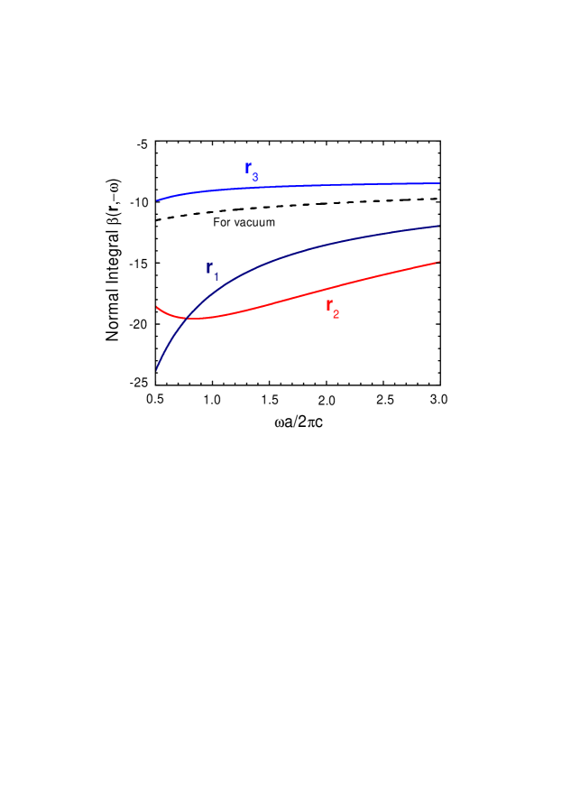
Figure 3: Normal integral $\beta({\bf r},-\omega)$ for three different positions in the photonic crystal. All parameters are the same as in Fig. 1. The dash line corresponds to the case of vacuum.

In PCs, the LSRF $g({\bf r},\omega^{\prime})$ displays dramatic fluctuations when the frequency $\omega^{\prime}$ varies for a given position. As an example, we demonstrate this in Fig. 1 for an 3D inverse-opal PC Wij without stacking faults Yannopapas . Thus, the principal integral $\beta({\bf r},\omega)$ $(\omega>0)$ should be very sensitive to the value of $\omega$, and the contribution to the integral comes mainly from the region near the frequency $\omega$. Figure 2 shows that $\beta({\bf r},\omega)$ is an oscillatory function of $\omega$. However, for the normal integral $\beta({\bf r},-\omega)$ $(\omega>0)$, the fluctuation in $g({\bf r},\omega^{\prime})$ are smoothed out after integration, and $\beta({\bf r},-\omega)$ is a slowly varying function of $\omega$, similar to the case of vacuum. In Fig. 3, we find a confirmation of this behavior of the function $\beta({\bf r},-\omega)$. Furthermore, it can be seen that in a PC the function $\beta({\bf r},-\omega)$ tends to the limit value of that in vacuum as the frequency $\omega$ grows. Therefore, the terms with $j>l$ in the right-hand side of Eq. (6) can be treated similar to the case of vacuum. If we consider $\bar{\omega}-\omega_{l}\gg 1$, then the PCs do not bring about appreciable changes in those terms with $j>l$ compared to the case of vacuum. Therefore, Eq. (6) can be approximated as follows

$$\omega-\omega_{l}-\Delta_{l}^{0}\simeq\sum_{j<l}\frac{\alpha_{lj}(\omega-\omega_{j})}{2\pi}{\cal P}\int^{\omega_{\rm op}}_{0}\frac{g({\bf r},\omega^{\prime})-\omega^{\prime}}{(\omega-\omega_{j}-\omega^{\prime})\omega^{\prime}}d\omega^{\prime}.$$ (9)

Equation (9) shows that, compared to the case of vacuum, inhomogeneous EM systems lead to an additional contribution to the Lamb shift that comes mainly from the real photon processes, rather than the virtual photon precesses, in contrast to the case of vacuum.

We now apply our result (9) to study the Lamb shift for a hydrogen atom in the inverse-opal PC. First, we obtain an interesting result that the PCs environment has no effect on the $2s$ state due to $\alpha_{2s1s}=0$; this result coincides with the prediction obtained earlier from the isotropic dispersion model John2 . However, for the $2p$ state, we have $\Delta^{0}_{2p}=0$ and $\alpha_{2p1s}\simeq 4\times 10^{-7}$. Numerical results for the Lamb shift of the $2p$ state are presented in Fig. 4. We find no level splitting, which differs our finding from the prediction of the isotropic model John2 . In addition, the Lamb shift depends strongly on not only the transition frequency but also on the atomic space position, different from dispersion models John2 ; Zhu2 ; Vats . The similar properties can also be found for the $3s$, $3p$, and $3d$ states.

Analyzing the results presented in Fig. 4, we notice that the Lamb shift can take very large positive or negative values and, therefore, it can be termed as a giant Lamb shift. Comparing the results for the PC with those for vacuum, we find that the Lamb shift may be enhanced in the PC by one or two orders of magnitude. Furthermore, it is significant to point out that the giant Lamb shift may occur for the transition frequency being either near or far away from the photonic band gap. The above-mentioned results are in contrast to the predictions based on dramatically simplified models John2 ; Zhu2 ; Vats ; Li . In Ref. Li , a PBG structure was simply treated as an averaged homogenous medium. This smooths out the contribution to the Lamb shift from real photon processes that play a key role in inhomogeneous systems. In the isotropic model John2 , $g({\bf r},\omega)\sim(\omega-\omega_{c})^{-1/2}/\omega$, that gives an infinite interaction between atom and photons at the band edge $\omega=\omega_{c}$ leading to the level splitting and anomalous Lamb shift. In the anisotropic model Zhu2 , $g({\bf r},\omega)\sim(\omega-\omega_{c})^{1/2}/\omega$, that leads to coupling interaction near the band edge being smaller than that in vacuum where $g({\bf r},\omega)=\omega$; it predicts much smaller Lamb shift than that in vacuum. In pseudogap model Vats , $g({\bf r},\omega)\sim\omega\{1-h\exp[(\omega-\omega_{c})^{2}/\sigma^{2}]\}$, that gives rise to small values of the Lamb shift near a pseudogap. Clearly, these models lose the main physical characteristics of the LSRF $g({\bf r},\omega)$ in realistic PCs that may result in the giant Lamb shift and other significant effects.

Based upon the position-dependent Lamb shift, we can suggest a possible experimental approach for verifying our theoretical predictions: if an assemble of atoms spreads randomly in PCs, the atoms at different positions have different values of the Lamb shift. Then the $l$-state levels of many atoms should form a $l$-state mini-band, similar to the velocity-dependent Doppler effect in atomic/molecular gases. This mini-band should be experimentally observable through the emission spectrum of these atoms.

In conclusion, we have developed a general formalism for calculating the Lamb shift for multi-level atoms. It is revealed that the real photon processes play a key pole in inhomogeneous dielectric structures. Our numerical results for atomic hydrogen in a 3D inverse-opal PC show that the Lamb shift may be enhanced remarkably by the PC environment. We have also predicted the existence of the Lamb shift mini-band for an assemble of atoms opening up possible ways for experimental observations. We believe our results provide a deeper insight into the theory of spontaneous emission in PCs and many applications such as the development of thresholdless lasers.

This work was supported by the Australian Research Council. The authors thank Kurt Busch, Judith Dawes, Martjin de Sterke, Sajeev John, Ross McPhedran, Sergei Mingaleev, and Kazuaki Sakoda for useful discussions and suggestions.

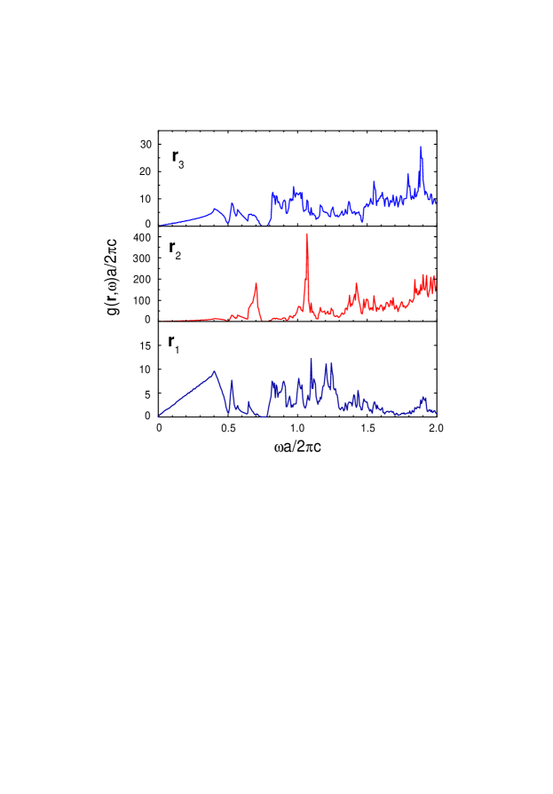
Figure 1: Local spectral response function $g({\bf r},\omega)$ for an atom placed at three different positions: ${\bf r}_{1}=(0,0,0)a$, ${\bf r}_{2}=(0.34,0,0)a$, and ${\bf r}_{3}=(0.24,0.24,0)a$ in the inverse-opal photonic crystal created by air spheres in a medium with $n=3.6$ and $f=0.74$; $a$ is the lattice spacing.

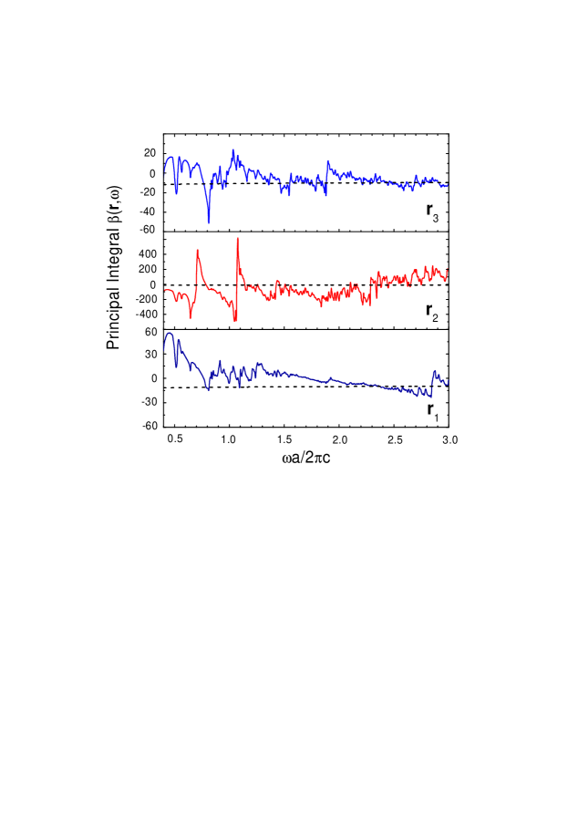
Figure 2: Principal integral $\beta({\bf r},\omega)$ for three different atomic positions in the photonic crystal. All parameters are the same as in Fig. 1. The dash line corresponds to the case of vacuum.

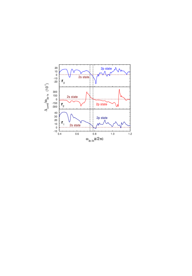
Figure 4: The Lamb shift of $2s$ and $2p$ states as a function of the lattice constant $a$ for atomic hydrogen located at three different positions in the photonic crystal. The Lamb shift of $2s$ state (the dashed lines) is the same as the value in vacuum. All parameters are the same as in Fig. 1. The frequency region between two dashed-dot lines is the photonic band gap.

References

- (1) []E–mail: xhw124@rsphysse.anu.edu.au
- (2) W. E. Lamb and R.C. Retherford, Phys. Rev. 72, 241 (1947).
- (3) H.A. Bethe, Phys. Rev. 72, 339 (1947).
- (4) G.W.F. Drake and R.B. Grimley, Phys. Rev. A. 8, 157 (1973); A. van Wijngaarden, J. Kwela, and G.W.F. Drake, ibid 43, 3325 (1991); A. van Wijngaarden, F. Holuj, and G.W.F. Drake, ibid 63, 012505 (2000).
- (5) S.G. Karshenboim, Zh. Eksp. Teor. Fiz. 103, 1105 (1993); K. Pachucki, Phys. Rev. Lett. 72, 3154 (1994); M. Eides and V. Shelyuto, Phys. Rev. A 52, 954 (1995).
- (6) V.A. Yerokhin, Phys. Rev. Lett. 86, 1990 (2001); V.A. Yerokhin, P. Indelicato, and V.M. Shabaev, Phys. Rev. Lett. 91, 073001 (2003); U.D. Jentschura et al., Phys. Rev. Lett. 90, 163001 (2003).
- (7) M.Y. Kuchiev and V.V. Flambaum, Phys. Rev. Lett. 89, 283002 (2002); A.I. Milstein, O.P. Sushkov, and I.S. Terekhov, Phys. Rev. Leet. 89, 283003 (2002).
- (8) M. Chaichian, M.M. Sheikh-Jabbari, and A. Tureanu, Phys. Rev. Lett. 86, 2716 (2001).
- (9) See, e.g., S. John, Phys. Today 44(5), 32 (1991).
- (10) K. Sakoda, Optical Properties of Photonic Crystals (Springer-Verlag, Berlin, 2001)
- (11) E. Yablonovitch, Phys. Rev. Lett. 58, 2059 (1987).
- (12) T. Quang et al., Phys. Rev. Lett. 79, 5238 (1997).
- (13) S.Y. Zhu, H. Chen, and H. Huang, Phys. Rev. Lett. 79, 205 (1997).
- (14) S. Bay, P. Lambropoulos, and K. Molmer, Phys. Rev. Lett. 79, 2654 (1997); Phys. Rev. A 55, 1485 (1997).
- (15) S. John and T. Quang, Phys. Rev. Lett. 74, 3419 (1995); ibid 76, 1320 (1996).
- (16) Xue-Hua Wang, Rongzhou Wang, Ben-Yuan Gu, and Guo-Zhen Yang, Phys. Rev. Lett. 88, 093902 (2002); E.P. Petrov et al., Phys. Rev. Lett. 81, 77 (1998).
- (17) Xue-Hua Wang, Ben-Yuan Gu, Rongzhou Wang, and Hong-Qi Xu, Phys. Rev. Lett. 91, 113904 (2003).
- (18) I. Alvarado–Rodriguez, P. Halevi, and A. S. Sanchez, Phys. Rev. E 63, 56613 (2001).
- (19) S. John and J. Wang, Phys. Rev. Lett. 64, 2418 (1990); Phys. Rev. B 43, 12772 (1991).
- (20) S. Y. Zhu et al., Phys. Rev. Lett. 84, 2136 (2000); Y. Yang and S. Y. Zhu, Phys. Rev. A 62, 013805 (2000)
- (21) N. Vats, S. John, and K. Busch, Phys. Rev. A 65, 043808 (2002)
- (22) Z.Y. Li and Y. Xia, Phys. Rev. B 63, 121305(R) (2001).
- (23) W.H. Louisell, Quantum Statistical Properties of Radiation (John Wiley & Sons, New York 1973).
- (24) K.M. Ho, C.T. Chan, and C.M. Soukoulis, Phys. Rev. Lett. 65, 3152 (1990); K.M. Leung and Y.F. Liu, ibid. 65, 2646 (1990); Z. Zhang and S. Satpathy, ibid. 65, 2650 (1990).
- (25) C. Cohen-Tannoudji, J. Dupont–Poc, and G. Grynberg, Atom–Photon Interactions: Basic Processes and Application (John Wiley & Sons, New York 1992).
- (26) P. Lambropoulos, G.M. Nikolopoulos, T.R. Nielsen, and S. Bay, Rep. Prog. Phys. 63, 455 (2000).
- (27) Rongzhou Wang, Xue-Hua Wang, Ben-Yua Gu, and Gou-Zhen Yang, Phys. Rev. B 67, 155114 (2003).
- (28) V.P. Bykov, Zh. Eksp. Teor. Fiz. 62, 505 (1972).
- (29) J.E.G.J. Wijnhoven and W. L. Vos, Science 281, 802 (1998).
- (30) V. Yannopapas, N. Stefanou, and A. Modinos, Phys. Rev. Lett 86, 4811 (2001).