The field inside a random distribution of parallel dipoles.

Abstract

We determine the probability distribution for the field inside a random uniform distribution of electric or magnetic dipoles. For parallel dipoles, simulations and an analytical derivation show that although the average contribution from any spherical shell around the probe position vanishes, the Levy stable distribution of the field is symmetric around a non-vanishing field amplitude. In addition we show how omission of contributions from a small volume around the probe leads to a field distribution with a vanishing mean, which, in the limit of vanishing excluded volume, converges to the shifted distribution.

The $z$-component of the field $F_{z}$ at the origin due to an electric or magnetic dipole located at $\boldsymbol{r}$ is given by the expression

$$F_{z}=C\frac{1}{r^{3}}\left((\hat{\boldsymbol{z}}\cdot\hat{\boldsymbol{n}})-3(\hat{\boldsymbol{r}}\cdot\hat{\boldsymbol{z}})(\hat{\boldsymbol{r}}\cdot\hat{\boldsymbol{n}})\right),$$ (1)

where $C=d/4\pi\varepsilon_{0}$ for an electric dipole $\boldsymbol{d}=d\hat{\boldsymbol{n}}$ and $C=\mu_{0}m/4\pi$ for a magnetic dipole $\boldsymbol{m}=m\hat{\boldsymbol{n}}$. $\hat{\boldsymbol{z}}$ and $\hat{\boldsymbol{r}}$ are unit vectors along the z-axis and $\boldsymbol{r}$, respectively. The field at a location within a random uniform distribution of many dipoles is a superposition of terms like the one in Eq.(1). The field component from a dipole parallel to the $z$-axis located at a distance $r$ and at a direction $\theta$ with respect to the $z$-axis is $C(1-3\cos^{2}\theta)/r^{3}$, and one sees that the average of this expression over directions in space vanishes for all distances $r$. It is hence surprising, that the field distribution in Fig. 1, obtained by numerical simulation, is symmetrical around a non-vanishing value of the field. We shall prove analytically that the distribution is a shifted Lorentzian, shown as the solid line in the figure, and that this is the mathematical limit of distribution functions which all have vanishing mean values but larger and larger variances.

The fields from electric and magnetic dipoles give rise to the most important interactions of neutral matter, and they play significant roles in atomic, molecular, and many-body physics. In the conclusion we shall list topics in current quantum gas and quantum information research where the present analysis may have important consequences.

Figure 1: The probability distribution for $g=F_{z}/F_{0}$, the scaled $z$-component of the field inside a random distribution of dipoles aligned along the $z$-axis. The symbols show the result of a numerical simulation (based on $10^{6}$ realizations of a system with $50.000$ individual dipoles, the uncertainty is represented by the line thickness), the solid curve is the exact Lorentzian solution for the probability distribution.

A typical distance between dipoles with a given density $\rho$ is $r_{0}=(3/4\pi\rho)^{1/3}$, and a corresponding typical field strength is $F_{0}=Cr_{0}^{-3}$. For notational convenience, we will rewrite Eq. (1) in terms of these typical values as

$$g=\frac{F_{z}}{F_{0}}=\left(\frac{r}{r_{0}}\right)^{-3}d(\hat{\boldsymbol{r}},\hat{\boldsymbol{n}}),$$ (2)

where $d(\hat{\boldsymbol{r}},\hat{\boldsymbol{n}})$ is the geometrical factor of Eq. (1).

To derive the distribution function $P_{N}(g)$ for the field component within a randomly distributed collection of $N$ dipoles we shall first derive the distribution $P_{1,N}(g)=P(g|r<N^{1/3}r_{0})$ for the contribution from a single dipole within a sphere of radius $N^{1/3}r_{0}$. The combined field due to $N$ dipoles within the same sphere is distributed according to the $N$-th order convolution product

$$P_{N}(g)=\int\delta(\sum_{i=1}^{N}g_{i}-g)\ \prod_{j=1}^{N}P_{1,N}(g_{j})\,dg_{j}.$$ (3)

The probability distribution $P_{1,N}$ is calculated as

$$P_{1,N}(g)=\left\langle{\int_{0}^{N^{1/3}r_{0}}\delta\left(g-\left(\frac{r}{r_{0}}\right)^{-3}d(\hat{\boldsymbol{r}},\hat{\boldsymbol{n}})\right)\frac{3r^{2}dr}{Nr_{0}^{3}}}\right\rangle,$$ (4)

where we explicitly integrate over the radial distribution of dipoles, and where $\left\langle{\cdot}\right\rangle$ denotes the expectation value with respect to the direction towards the dipole. The expression readily incorporates also an average over possibly varying directions $\hat{\boldsymbol{n}}$ of the individual dipoles to be only briefly considered below. By a simple substitution, we rewrite Eq. (4) as

$$P_{1,N}(g)=\frac{1}{Ng^{2}}\,D(Ng),$$ (5)

where $D(g)$ is a geometrical factor which depends only on the distribution of $d$:

$$D(g)=\left\langle{\left|d(\hat{\boldsymbol{r}},\hat{\boldsymbol{n}})\right|\int^{1}_{0}\delta(u-\frac{d(\hat{\boldsymbol{r}},\hat{\boldsymbol{n}})}{g})du}\right\rangle.$$ (6)

We observe the simple scaling of the probability distribution for the field of a single dipole in a large volume holding on average $N$ dipoles: $P_{1,N}(g)=NP_{1,1}(Ng)$.

For dipoles parallel to the $z$-axis, $d(\hat{\boldsymbol{r}},\hat{\boldsymbol{n}})$ attains the value

$$d^{({p})}(\theta)=1-3\cos^{2}\theta,$$ (7)

from which we find by integration over solid angles that

$$D^{({p})}(g)=\frac{1}{3\sqrt{3}}\begin{cases}2-(2+g)\sqrt{1-g}&\text{if $-2<g<1$,}\\ 2&\text{otherwise.}\end{cases}$$ (8)

The fact that $D^{({p})}(g)$ assumes a constant value of $D^{({p})}_{\infty}=2/3\sqrt{3}\approx 0.3849$ for $|g|>2$ follows from (6) because $|d|$ is bounded by $2$ and it provides $P_{1,N}$ with algebraic tails proportional to $g^{-2}$. This is illustrated in Fig. 2, where $P_{1,1}^{({p})}$ is compared to the distribution corresponding to a step approximation of $D^{({p})}$ with the same limiting value:

$$D^{({\theta})}(g)=\begin{cases}D_{\infty}\qquad&\text{for $|g|>2D_{\infty}$}\\ 0&\text{otherwise,}\end{cases}$$ (9)

where the position of the edge is determined by the normalization of $P_{1,1}(g)$.

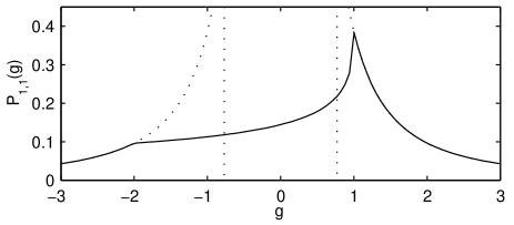
Figure 2: The probability distribution $P^{({p})}_{1,1}(g)=g^{-2}D^{({p})}(g)$ for the field contribution from a single dipole parallel to the $z$-axis. The dotted curve is based on the step approximation $D^{({\theta})}(g)$, with the same asymptotic values as $D^{({p})}(g)$.

Due to the $g^{-2}$ algebraic tails, the distribution $P_{1,1}$ has a divergent variance and an ill-defined mean value. This type of problems is addressed by generalized (Levy) statistics, see e.g. Feller (1966), and the form of the bulk distribution $P_{\infty}\equiv\lim_{N\to\infty}P_{N}$ can be calculated by the generalized central limit theorem, see e.g. chapter 17 of Fristedt and Gray (1996). We will, however, calculate $P_{\infty}$ directly as the limit of $P_{N}$ to establish a formalism where the effect of an excluded volume can also be obtained.

The simple scaling relation between $P_{1,N}(g)$ and $P_{1,1}(g)$ allows us to express $P_{N}$ in terms of $P_{1,1}$ by rewriting the convolution Eq. (3) in Fourier space as

$$P_{N}(g)=\int e^{ikg}\left(\operatorname{\tilde{P}}_{1,1}(\tfrac{k}{N})\right)^{N}\frac{dk}{2\pi},$$ (10)

where $\tilde{\cdot}$ denotes the Fourier transform: $\tilde{f}(k)=\int e^{-ikg}f(g)dg$. Eq. (10) implies that to determine $P_{N}$ in the limit of $N\to\infty$ we must know the dependence of $\operatorname{\tilde{P}}_{1,1}(k)$ for small $k$. We first rewrite $\operatorname{\tilde{P}}_{1,1}(k)$ as

$$\begin{split}\operatorname{\tilde{P}}_{1,1}(k)=&\int e^{-ikg}g^{-2}D^{({\theta})}(g)dg\\ &+\int e^{-ikg}g^{-2}\left(D(g)-D^{({\theta})}(g)\right)dg,\end{split}$$ (11)

where the first term is conveniently rewritten as

$$1-2|k|D_{\infty}\left(\frac{\pi}{2}-\int_{0}^{2|k|D_{\infty}}\frac{1-\cos(t)}{t^{2}}dt\right).$$ (12)

In a small $k$ expansion of the second integral of (11), the $0^{\text{th}}$ order term vanishes since $g^{-2}D(g)$ and $g^{-2}D^{({\theta})}(g)$ are both normalized. $D$ and $D^{({\theta})}$ are equal for all $|g|>2$ and since $D^{({\theta})}$ is even, the $1^{\text{st}}$ order term yields $-ikg_{c}$ with $g_{c}$ defined as

$$g_{c}=\int_{-g_{0}}^{g_{0}}gP_{1,1}(g)dg,$$ (13)

for any $g_{0}>2$. Collecting the two parts we find that $\operatorname{\tilde{P}}_{1,1}(k)=1-\pi D_{\infty}|k|-ikg_{c}+\operatorname{\mathcal{O}}(k^{2})$. Insertion of the expression for $D^{({p})}(g)$ leads to the value

$$g_{c}^{({p})}=\frac{2}{9}\left(3+\sqrt{3}\log\frac{\sqrt{3}-1}{\sqrt{3}+1}\right)\approx 0.1598.$$ (14)

To calculate the limit of $P_{N}$ for $N\to\infty$, we rewrite (10) as $\log(\operatorname{\tilde{P}}_{N}(k))=N\log\operatorname{\tilde{P}}_{1,1}(k/N)$. Since $\operatorname{\tilde{P}}_{1,1}(0)=1$ and $\log(1+u)=u+\operatorname{\mathcal{O}}(u^{2})$, the leading terms of the series expansion of $(\operatorname{\tilde{P}}_{1,1}(k)-1)$ will dominate in the limit of $N\to\infty$, so that

$$\log(\operatorname{\tilde{P}}_{\infty}(k))=-\pi D_{\infty}|k|-ig_{c}k,$$ (15)

from which the limiting distribution follows directly:

$$P_{\infty}(g)=\frac{1}{\pi}\frac{\Gamma}{\Gamma^{2}+(g-g_{c})^{2}}.$$ (16)

This Lorentzian with a half width of $\Gamma=\pi D_{\infty}$ and a displacement of $g_{c}$ is in excellent agreement with our numerical simulations shown in Fig. 1. The half width $\pi D^{({p})}_{\infty}F_{0}\approx 5.065\,C\rho$ and central value $g^{({p})}_{c}F_{0}\approx 0.6692\,C\rho$ of the field distribution $P(F_{z})$ are both proportional to the dipole density $\rho$, and their ratio is independent of $\rho$.

The shift of the most probable value with respect to zero is surprising when one considers the vanishing mean contribution from any spherical shell around the origin, but it is less surprising when one observes the probability distribution for the single dipole contribution, shown in Figure 2. This distribution is indeed suggestive of a shift, but its mean is ill-defined, and (13) provides the proper procedure to obtain $g_{c}$ from $P_{1,1}(g)$.

For completeness we note that, in the case of randomly oriented dipoles, the factor $d(\hat{\boldsymbol{r}},\hat{\boldsymbol{n}})$ is given by

$$d^{({r})}=\sin\theta_{1}\sin\theta_{2}\sin\phi-2\cos\theta_{1}\cos\theta_{2},$$ (17)

where $\theta_{1}$ is the direction of $\hat{\boldsymbol{r}}$, $\theta_{2}$ is the angle between $\hat{\boldsymbol{r}}$ and $\hat{\boldsymbol{n}}$, and $\phi$ represents the rotations of $\hat{\boldsymbol{n}}$ around $\hat{\boldsymbol{r}}$. Integration over these angles with the appropriate probability measure $\sin(\theta_{1})\sin(\theta_{2})d\theta_{1}d\theta_{2}d\phi/8\pi$ yields an even function $D^{({r})}(g)$ with the asymptotic limit $D^{({r})}_{\infty}=\frac{1}{4}+\frac{\sqrt{3}}{24}\sinh^{-1}(\sqrt{3})\approx 0.3450$, implying a Lorentzian distribution with a half width $\Gamma=\pi D^{({r})}_{\infty}\simeq 1.083$ centered at zero field. This is in agreement with work by Stoneham Stoneham (1969), who considered a variety of line broadening mechanisms in solids, and identified a Lorentzian line as the result of interaction of a single molecule with dislocation dipoles. More recently Barkai et al. (2000) Lorentzian line shapes were measured for molecules embedded in low temperature glass with a low-density distribution of dynamical defects. These results were interpreted in terms of Levy stable distributions.

If the algebraic tails of $P_{1,1}$ are truncated by some mechanism, the distributions have finite variance, and our naive estimates of mean values will be valid due to the central limit theorem. To investigate whether such a truncation entirely removes the more spectacular effect identified above, we shall compute the field distribution in the case where we will not allow any dipoles inside an excluded volume in the form of a sphere of volume $\epsilon/\rho$ centered at the origin. Note that $\epsilon$ is the average number of dipoles that would have been found in the excluded volume. The symbols in Fig. 3 show the results of simulations performed with dipoles put uniformly at random around the origin but outside such excluded volumes, and as we reduce the excluded volume we observe that the probability distributions converge towards the shifted Lorentzian. The generalized central limit theorem which applies for $\epsilon=0$ and $\epsilon\to\infty$ deals with the convergence of the distribution function for a sum of more and more random variables which all have the same individual distribution after a suitable rescaling. Such rescaling is not possible for intermediate values of $\epsilon$, which thus require a direct calculation of $P_{\infty}(\epsilon,g)$.

We consider the field contribution from a single dipole placed at random in a spherical shell with outer radius $(N+\epsilon)^{1/3}r_{0}$ and inner radius $\epsilon^{1/3}r_{0}$. Parametrizing the radius by $x=(r/r_{0})^{3}$, the mean number of atoms populating the sphere with radius $r$, we have by Bayes rule and the additivity of probabilities of disjoint events that $P(\epsilon<x<N+\epsilon)P(g|\epsilon<x<N+\epsilon)=P(x<N+\epsilon)P(g|x<N+\epsilon)-P(x<\epsilon)P(g|x<\epsilon)$, where the first factors are simply the probabilities that a single particle is found in the specified regions of space, and, e.g., $P(x<(N+\epsilon))/P(x<\epsilon)=(N+\epsilon)/\epsilon$. Taking the Fourier transform with respect to $g$ and noting that $\operatorname{\tilde{P}}(k|x<x_{i})=\operatorname{\tilde{P}}_{1,1}(k/x_{i})$, we obtain the following relation between the Fourier transformed probabilities

$$N\,\operatorname{\tilde{P}}(k|\epsilon<x<N+\epsilon)=(N+\epsilon)\operatorname{\tilde{P}}_{1,1}(\tfrac{k}{N+\epsilon})-\epsilon\operatorname{\tilde{P}}_{1,1}(\tfrac{k}{\epsilon}).$$

We are interested in the probability $P_{N}(\epsilon,g)$ that the contributions from $N$ dipoles, all having $\epsilon<x<N+\epsilon$, add up to the value $g$. Performing the convolution in Fourier space we find that $\log\operatorname{\tilde{P}}_{N}(\epsilon,k)=N\log\operatorname{\tilde{P}}(k|\epsilon<x<N+\epsilon)$, and for $N\to\infty$ we have

$$\log\operatorname{\tilde{P}}_{\infty}(\epsilon,k)=\log\operatorname{\tilde{P}}_{\infty}(k)-\epsilon(\operatorname{\tilde{P}}_{1,1}(\tfrac{k}{\epsilon})-1).$$ (18)

As shown by Fig. 3 this expression, which can be evaluated numerically, is in excellent agreement with numerical simulations.

$|\operatorname{\tilde{P}}_{1,1}|<1$, and, by (15), the term $\log\operatorname{\tilde{P}}_{\infty}(k)$ will dominate Eq. (18) for $k>\epsilon$, in agreement with our expectation that $P_{\infty}(\epsilon,g)$ should approach $P_{\infty}(g)$ for $\epsilon\to 0$. To consider the limit of $\epsilon\to\infty$ we continue the series expansion of $\operatorname{\tilde{P}}_{1,1}$ to find $\log\operatorname{\tilde{P}}^{({p})}_{\infty}(\epsilon,k)=-2/5\,\epsilon^{-1}k^{2}-4i/105\,\epsilon^{-2}k^{3}+\epsilon\operatorname{\mathcal{O}}((k/\epsilon)^{4})$. Since the leading term of this expansion will dominate for $\epsilon\gg 1$, we conclude that $P_{\infty}(\epsilon,g)$ asymptotically approaches a Gaussian distribution with variance $\text{Var}(g)=4/5\,\epsilon^{-1}$.

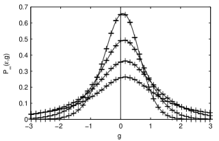
Figure 3: Distribution of $g$ for the case of dipoles parallel to the $z$-axis when an excluded volume of size $\epsilon/\rho$ is introduced. Solid lines show the distribution $P_{\infty}(\epsilon,g)$ given by (18), for $\epsilon=0$, $0.4$, $1$, and $2$ in order of increasing maximum densities. Data markers are the result of numerical simulations. The distributions have vanishing mean for all values of $\epsilon>0$, yet they approach the shifted Lorentzian, corresponding to $\epsilon=0$.

In summary, we have identified a shifted Lorentzian distribution as the probability distribution for the total field inside a random distribution of dipoles, and we have identified a family of distributions for the case where dipoles are not permitted inside an excluded volume around the origin. These distributions have vanishing mean, and they converge to Gaussian distributions in the limit of large excluded volumes and towards the Lorentzian in the case of small excluded volumes. It is not an inconsistency of our results that the shifted Lorentzian is approached by distributions with vanishing mean: a Lorentzian can be ascribed any mean value depending on how the upper and lower limits are taken in the integral over the distribution. There is in fact reason to emphasize that the common procedure of fitting a spectrum to a Lorentzian may be quite misleading if one tries to interpret a frequency shift as the mean value of a possible perturbation of the energy of the system.

The emergence of a non-vanishing field as the most likely result of the surroundings of any given dipole, could have consequences for material properties. The properties of a conventional ferromagnet are controlled by an interplay of Coulomb forces and the Pauli exclusion principle for electrons, which may be conveniently represented by a spin-spin interaction term, but in novel materials, such as recently produced carbon-nanofoams phy (2004), the actual interaction between separated magnetic dipoles may be an important ingredient in the understanding of their collective properties.

Heteronuclear molecules with permanent electric dipole moments have been trapped Bethlem et al. (2000) and experiments are planned with atomic species with particularly high magnetic dipole moments Góral et al. (2000); Martikainen et al. (2001); Giovanazzi et al. (2002) to study polar degenerate gases and new kinds of order and collective dynamics Yi and You (2000); Santos et al. (2000); Baranov et al. (2002); Damski et al. (2003). Mean-field approaches in dipolar degenerate quantum gases may of course be questionable if the mean field itself is not well defined. Our work suggest that a critical examination of this issue is necessary.

Highly excited Rydberg atoms in electric and magnetic fields interact strongly Fioretti et al. (1999), and fast quantum computing Jaksch et al. (2000) and single photon generating devices Lukin et al. (2001) have been suggested based on the energy shifts in atoms caused by the excitation of nearby atoms. Rare-earth ions in crystals have excited states with permanent electric dipole moments, and proposals exist for quantum computing within such a system which are also based on large Ohlsson et al. (2002) or small Longdell and Sellars (2003) shifts in absorption frequency of target ions caused by excitation of a nearby control-ion. In the rare-earth system Lorentzian broadening of spectrally hole burnt structures has been observed when ions at different frequencies are excited Nilsson et al. (2002), and we imagine that this can be an ideal system to study the broadening and the shift systematically, as the density of perturbing dipoles can be varied by the exciting laser system.

Extension of the analysis, e.g., to time-dependent fields and to higher order multipole fields seems very interesting. Von Neuman and Chandrasekhar considered the fluctuating gravitational forces in a stellar medium, see Chandrasekhar (1943). As a curiosity we note that the time derivative of these forces at any given time behaves like a sum of dipole fields, and hence a massive object moving through a static random mass distribution may experience a force with a time derivative given by the shifted Lorentzian.