Violation of Bell’s inequality for continuous variables

Abstract

We construct a wide class of bounded continuous variables observables that lead to violations of Bell inequalities for the EPR state and give an intuitive Wigner function explanation how to predetermine which operators won’t ever exceed the bounds given by local theories.

1 Introduction

Bell’s inequality was derived and tested for entangled system of two qubits (polarization or spin) photon ; aspect ; weihs ; 10km ; ion ; atom . Recent investigations have been dealing with systems described by continuous variables (CV) kluw such as the original Einstein-Podolsky-Rosen (EPR) example or entangled pairs of photons generated in non degenerate optical parametric amplification (NOPA). A simple way of implementing Bell measurements on CV systems is to use dichotomic (bounded by $\pm 1$) observables. Recent examples of such observables are the parity operator BW2 ; BW3 or CV spin operators chen . It is the purpose of this work to give a wide class of quantum observables that can be implemented into correlation measurements of entangled states. We show that such bounded operators will often have quite different properties in the Wigner representation – the representation that provides a fundamental link between classical and quantum physics. The Wigner function gives a natural phase-space framework in which the relation between local realism and quantum probability rules can be formulated and studied. The original EPR wave function is a Gaussian state with a nonnegative Wigner function, which can be interpreted as a hidden phase-space probability distribution. As we have already mentioned, the main goal of this paper is to construct a wide class of such bounded continuous variables observables that will lead to violations of Bell inequalities for the EPR state.

The paper is organized as follows: Sections 2 and 3 provide an introduction to the Wigner representation of quantum correlations, its connection with local theories and the CV form of the EPR state. In Section 4 we introduce a class of bounded observables and choose from them certain representatives that realize the Pauli algebra. The physical interpretation of these operators is presented in Section 5. The final Section 6 shows explicitly that some of these operators lead to a violation of Bell’s inequality. Results presented there were obtained either analytically or by rather simple numerics. Concluding remarks are offered in Section 7.

2 Entanglement in the Wigner representation

As an example let us probe a two-party entangled system, described by a non separable density operator $\rho$, for correlations. The probing of the entanglement can be achieved by a joint measurement performed by Alice and Bob using local observables $A$ and $B$. In this measurement, Alice and Bob measure a correlation $\langle A,B\rangle=\mathrm{Tr}\left\{(A\otimes B)\rho\right\}$. Using Wigner functions we can write this quantum correlation as

$$\langle A,B\rangle=\int(d\lambda_{a})(d\lambda_{b})W_{A}(\lambda_{a})\,W_{B}(\lambda_{b})\,W_{\rho}(\lambda_{a},\lambda_{b})\,,$$ (1)

where $(d\lambda_{a})$, $(d\lambda_{b})$ are properly normalized measures of the phase space variables $(q_{a},p_{a})$ and $(q_{b},p_{b})$, respectively. The three Wigner functions correspond to the observables $A$, $B$ (associated with Alice and Bob) and to the entangled state $\rho$. This formula has a remarkable structure of a local hidden variable theory if one entertains the association that $W_{A}$, $W_{B}$ correspond to “hidden” predetermined values of operators $A,\,B$, and $W_{\rho}(\lambda_{a},\lambda_{b})$ is a genuine local probability distribution function of the hidden variables.

From these correlation we can form the following Bell combination:

$${\mathcal{B}}=\langle A,B\rangle+\langle A,B^{\prime}\rangle+\langle A^{\prime},B\rangle-\langle A^{\prime},B^{\prime}\rangle\,.$$ (2)

In the local hidden variables theory Bell’s inequality $|{\mathcal{B}}|\leq 2$ should be satisfied if these observables fulfill the boundary conditions $|A|\leq 1$ and $|B|\leq 1$. For systems described by continuous variables, the selection of these variables is not as obvious as in the case of measurements performed on entangled qubits. This inequality can be treated as a test dividing purely quantum phenomena from those that can by explained by deterministic models. A violation of the Bell’s inequality (2) means that the effect we study requires a quantum description.

3 The EPR state

As an example of an entangled state leading to quantum CV correlations (1), we use a two-mode squeezed state. It is well known that the CV form of the EPR state can be generated in a non degenerate optical parametric amplification involving two modes of the radiation field kimble ; kimble2 . The wave function of such a pure quantum state $\rho=\bigl{|}\Psi\bigr{\rangle}\bigl{\langle}\Psi\bigr{|}$ has the Schmidt decomposition

$$|\Psi\rangle =\frac{1}{\cosh r}\sum_{n=0}^{\infty}(\tanh r)^{n}|n,n\rangle=$$ (3)

$$=\frac{1}{\sqrt{1+\langle n\rangle}}\sum_{n=0}^{\infty}\bigg{(}\frac{\langle n\rangle}{1+\langle n\rangle}\bigg{)}^{\frac{n}{2}}|n,n\rangle\,,$$

where $\langle n\rangle$ is the mean number of photons in each mode and $r$ denotes the squeezing parameter. These two parameterizations are connected by the relation $\langle n\rangle=\sinh^{2}r$. In the limit of $\langle n\rangle\rightarrow\infty$, the two-mode squeezed state becomes the original EPR state. The Wigner function of this state is given by

$$4\pi^{2}\,W_{\Psi}(q_{a},p_{a},q_{b},p_{b})$$ (4)

$$=\exp{\bigl{(}-(1+2\langle n\rangle)(p_{a}^{2}+p_{b}^{2})-4\sqrt{\langle n\rangle(\langle n\rangle+1)}p_{a}p_{b}\bigr{)}}$$

$$\times\exp{\bigl{(}-(1+2\langle n\rangle)(q_{a}^{2}+q_{b}^{2})+4\sqrt{\langle n\rangle(\langle n\rangle+1)}q_{a}q_{b}\bigr{)}}\,.$$

As it has been mentioned in the Introduction, the nonnegative Wigner function of the EPR state can be interpreted as a probability distribution of CV local realities.

It is worth noticing that this is a unique case when the Wigner function is exactly equal to the product of the probabilities in the position and momentum representations,

$$W_{\Psi}(q_{a},p_{a},q_{b},p_{b})=\frac{1}{(2\pi)^{2}}|\tilde{\Psi}(p_{a},p_{b})|^{2}|\Psi(q_{a},q_{b})|^{2}.$$ (5)

The factors are, of course, the marginal probabilities as obtained from the wave functions implied by Eq. (3),

$$\Psi(q_{a},q_{b})=\frac{1}{\sqrt{\pi}}e^{-(\langle n\rangle+\frac{1}{2})(q_{a}^{2}+{q_{b}}^{2})+2\sqrt{\langle n\rangle(1+\langle n\rangle)}q_{a}q_{b}},$$

$$\widetilde{\Psi}(p_{a},p_{b})=\sqrt{\pi}e^{-(\langle n\rangle+\frac{1}{2})(p_{a}^{2}+{p_{b}}^{2})-2\sqrt{\langle n\rangle(1+\langle n\rangle)}p_{a}p_{b}},$$

a consequence of the fact that the state considered is a Gaussian state with no position-momentum correlation between the two particles. We stress that it is really an untypical situation and the Wigner function here has an even more intuitive interpretation than usually.

The Wigner function of the entangled CV state can be used to describe the correlations between massive particles formed in a breakup process, or for clouds of cold atoms.

4 Bounded observables

Our goal is to construct quantum observables for Alice and Bob that are bounded by $\pm 1$ . For Alice we introduce a class of quantum observables of the form

$$A=\int dq\,a_{\epsilon}(q)\bigl{|}q\bigr{\rangle}\bigl{\langle}\epsilon q\bigr{|}\,$$ (6)

in the position representation, where $\epsilon\neq 0$ is a real parameter and $a_{\epsilon}(q)$ is a function of $q$. In the same way one can construct quantum observables for Bob.

This operator is hermitian ($A=A^{\dagger}$) if $\epsilon=\pm 1$ and

$$a_{\epsilon}(q)=a^{\ast}_{\epsilon}(\frac{q}{\epsilon})\,.$$ (7)

In this case we have $a_{+}(q)=a^{\ast}_{+}(q)$ or $a_{-}(q)=a_{-}^{\ast}(-q)$. The condition that this observable has a sharp bound, $A^{2}=1$, is satisfied if $a_{\epsilon}(q)a_{\epsilon}(\epsilon q)=1\,.$

The Wigner functions of these dichotomic operators with $\epsilon=\pm 1$ are

$$W_{A_{a_{+}}}(q,p) = \frac{1}{2\pi}a_{+}(q)\,,$$

$$W_{A_{a_{-}}}(q,p) = \frac{1}{2}\delta(q)\int\frac{d\xi}{2\pi}e^{ip\xi}\,a_{-}(\frac{\xi}{2})\,,$$ (8)

where we recognize in the last expression the Fourier transform of $a_{-}(q)$. In the case of $\epsilon=-1$, the corresponding Wigner function is never bounded, leading to a possible violation of the Bell inequalities. The simplest example of such an observable $A$ is the parity operator $\mathbb{P}$,

$$\mathbb{P}=\int dq\bigl{|}q\bigr{\rangle}\bigl{\langle}-q\bigr{|},$$ (9)

corresponding to $a_{-}(q)=1$. The Wigner function of this observable is

$$W_{\mathbb{P}}(q,p)=\frac{1}{2}\delta(q)\delta(p).$$ (10)

This dichotomic operator has been used recently to probe Bell inequalities for systems described by continuous variables BW2 ; BW3 .

Another simple example of a dichotomic operator is $a_{+}(q)=\mathrm{sgn}(q)$, corresponding to the sign operator $\mathbb{S}$,

$$\mathbb{S}=\int dq\,\mathrm{sgn}(q)\bigl{|}q\bigr{\rangle}\bigl{\langle}q\bigr{|}\,.$$ (11)

The corresponding Wigner function

$$W_{\mathbb{S}}(q,p)=\frac{1}{2\pi}\mathrm{sgn}(q)$$ (12)

is bounded and no violation of Bell inequalities should be expected. This example shows that the quantum nonlocality of the EPR state cannot be revealed by measuring quadrature components.

As another example, let us consider a function $a_{-}(q)=i\,\mathrm{sgn}(q)$. This function defines a hermitian operator that we shall call the parity inversion,

$$\mathbb{R}=i\int dq\,\mathrm{sgn}(q)\bigl{|}q\bigr{\rangle}\bigl{\langle}-q\bigr{|}\,.$$ (13)

The Wigner function of this observable is unbounded:

$$W_{\mathbb{R}}(q,p)=-\frac{1}{2}\delta(q)\mathcal{P}\frac{1}{p}\,,$$ (14)

($\mathcal{P}$ denotes the Cauchy principal value). Certainly this singular and unbounded function can be used to exhibit the nonlocality of the EPR state.

The three hermitian operators that we have introduced satisfy the commutation relations for the Pauli matrices,

$$[\mathbb{S},\mathbb{R}]=2i\mathbb{P},\ [\mathbb{P},\mathbb{S}]=2i\mathbb{R},\ [\mathbb{R},\mathbb{P}]=2i\mathbb{S}\,.$$ (15)

Different in form representations of the commutation relations presented above have been given in the recent literature chen ; fiurasek ; gour .

It is well known that the phase-space shift of an observable can be implemented with the help of the local displacement operator $D(q,p)$ that is familiar from the theory of coherent states. In the following section we will use such shifts in order to form the Bell combination. For Alice and Bob we introduce shifted operators $A(\alpha)=D(\alpha)AD^{\dagger}(\alpha)$ and $B(\beta)=D(\beta)AD^{\dagger}(\beta)$, where the two complex numbers $\alpha$ and $\beta$ characterize the phase space shifts in Alice’s and Bob’s position and momentum $(q,p)$. These parameters are the CV analogues of the polarization settings for qubits.

For an unsharp bound of the observables, the condition for $\epsilon$ is less restrictive. We will give examples of such unsharp functions at the end of this paper.

5 Measurements by Alice and Bob

The expectation values of $\mathbb{P}$, $\mathbb{R}$, $\mathbb{S}$ provide their physical interpretation (or at least operational meaning associated with position measurements):

$$\bigl{\langle}\mathbb{P}\bigr{\rangle}=\int\,dq\,\Psi^{*}(q)\Psi(-q)\,,$$

$$\bigl{\langle}\mathbb{S}\bigr{\rangle}=\int_{R_{+}}\,dq\,|\Psi(q)|^{2}-\int_{R_{-}}\,dq\,|\Psi(q)|^{2}\,,$$ (16)

$$\bigl{\langle}\mathbb{R}\bigr{\rangle}=i\biggl{(}\int_{R_{+}}\,dq\,\Psi^{*}(q)\Psi(-q)-\int_{R_{-}}\,dq\,\Psi^{*}(q)\Psi(-q)\biggr{)}.$$

According to the equations above the expectation value of $\mathbb{P}$ is (up to the normalization factor) equal to the Wigner function value at the origin, $W(0,0)$. Measurements of the parity operator $\mathbb{P}$ can be implemented for the electromagnetic field by using photon counting, or by measuring the atomic inversion in a micromaser cavity bge . For atomic wave packets or for cold atoms, a parity measurement can be performed by a measurement of the current position of the particle relative to a fixed origin ulm .

The expectation value of $\mathbb{S}$ is an “inversion of probability” a difference between probabilities of finding a particle in the positive and negative side of the position axis, which can be associated with measurements of quadrature components.

Similarly the expectation value of $\mathbb{R}$ corresponds to an “inversion of parity” i.e., a difference between parity measurements on the positive and negative side of the real axis. Specific and operational implementations of these measurements for photons and atoms are under investigation.

6 Violations of Bell inequalities

6.1 Displaced $\mathbb{R}$ Operators

In this section we investigate the violation of the Bell inequality by the shifted parity inversions $\mathbb{R}$ for Bob and Alice. We introduce the following correlation function:

$$E(\alpha,\beta)=\bigl{\langle}\Psi\bigr{|}\mathbb{R}(\alpha)\otimes\mathbb{R}(\beta)\bigl{|}\Psi\bigr{\rangle}$$ (17)

Properly chosen combination of $E(\alpha,\beta)$ violates Bell’s inequality. In the simple case when displacement parameters are real (e.g. $\alpha=\mathrm{Re}(\alpha)=q$ and $\beta=\mathrm{Re}(\beta)=q^{\prime}$) the correlation can be evaluated analytically and is given by

$$E(q,q^{\prime})=\frac{2}{\pi}{\mathrm{arctan{(2\sqrt{\langle n\rangle(1+\langle n\rangle)})}}}\;$$ (18)

$$\;\times\,e^{-(1+2\langle n\rangle)\left(q^{2}+{q^{\prime}}^{2}\right)+4\sqrt{\langle n\rangle(1+\langle n\rangle)}qq^{\prime}}.$$

From this correlation function we form the Bell combination (2)

$$B(d,\langle n\rangle)=E(0,0)+E(0,d)+E(-d,0)-E(-d,d)\,,$$ (19)

where $d$ and $0$ are the only distance parameters involved in the settings. The parameter $\langle n\rangle$ characterizes the EPR state. The Bell combination (19) is depicted in Figure 1, and a clear violation of the bound imposed by local theories can be seen for various values of $d$ and $\langle n\rangle$.

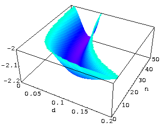
Figure 1: Plot of the expression $B(d,\langle n\rangle)$ from Eq. (19) for parity inversions. Only values that exceed the bound imposed by local theories are shown.

If a momentum shift of the parity inversion operators is performed in addition, no analytical expression for the correlation can be obtained. Numerical calculations show, however, that for such shifts a violation of Bell’s inequality is also possible. Figure 2 shows expression (2) for such composed position and momentum shifts,

$$E(0,0)+E(0,d+i\frac{d}{2})+E(-d+i\frac{d}{2},0)-E(-d+i\frac{d}{2},d+i\frac{d}{2}).$$ (20)

The violation is still noticeable, although for a slightly smaller range of the shift parameters $d$.

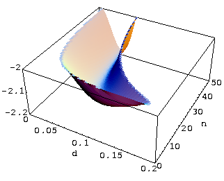
Figure 2: Plot of $B$ from Eq. (20). Again, only values that exceed the bound imposed by local theories are shown.

6.2 Displaced unsharp observables

When defining the dichotomic operators forming the CV version of the Pauli algebra we emphasized that it involved an arbitrary choice. In general, one can introduce an infinite number of operators with similar properties and probably the only limit would appear when taking care of their clear physical interpretation. The parity inversion operator $\mathbb{R}$ was based on a dichotomic $\mathrm{sgn}(q)$ function. In this part of the paper we shall relax this condition and instead of the discontinuous function ${\mathrm{sgn}}(q)$ take a family of functions $f_{l}(q,s)$ ($l=1,\,2,...$) that are not dichotomic but in some limit of parameter $s$ represent the sign function. Defining

$$\mathbb{R}_{l}=i\int dq\,f_{l}(q,s)|q\rangle\langle-q|$$

we obtain operators that may lead to violations of Bell’s inequality. The simplest examples of such sequences are $\,f_{1}(q,s)=\tanh(sq)\,$ or

$$f_{2}(q,s)=\left\{\begin{array}[]{lll}(1-e^{-sq})&\mathrm{for}&q\geq 0\\ (e^{sq}-1)&\mathrm{for}&q\leq 0,\end{array}\right.$$

and

$$f_{3}(q,s)=\left\{\begin{array}[]{lll}(1-e^{-sq^{2}})&\mathrm{for}&q\geq 0\\ (e^{-sq^{2}}-1)&\mathrm{}&q\leq 0.\end{array}\right.$$

Figure 3 reports results obtained for Bell combination calculated with $f_{1}(q,s)=\tanh(sq)$.

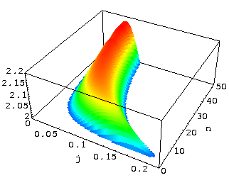
Figure 3: Combination (2) as depicted in Figure 1 – except that instead of ${\mathrm{sgn(q)}}$ we have used here $\tanh(100q)$

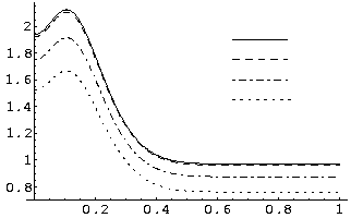
Figure 4: Cross-section of Figure 3 for $\langle n\rangle$=10 and values of parameter $s$ equal to $100$, $10$, $2$, and $1$, respectively.

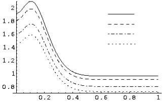
Figure 5: Similar cross-section as depicted in Figure 4 ($\langle n\rangle$=10 and $s$ equal to $100$, $10$, $2$, and $1$) obtained for $f_{3}(q,s)$.

The Wigner functions of the corresponding $\mathbb{R}_{l}$ are of the form

$$W_{f_{1}}\sim\delta(q)\bigg{\{}{\cal{P}}\big{(}\frac{1}{p}\big{)}-\frac{i}{2s}\bigg{[}\frac{2s}{p}+\frac{2\pi}{e^{-\frac{\pi p}{2s}}-e^{\frac{\pi p}{2s}}}\bigg{]}\bigg{\}},$$

$$W_{f_{2}}\sim\delta(q)\bigg{\{}{\cal{P}}\big{(}\frac{1}{p}\big{)}-\frac{s}{s^{2}+p^{2}}\bigg{\}},$$

$$W_{f_{3}}\sim\delta(q)\bigg{\{}{\cal{P}}\big{(}\frac{1}{p}\big{)}-\frac{\sqrt{\pi}}{2s}\mathrm{erf}\big{(}\frac{ip}{2s}\big{)}\bigg{\}}.$$

In the limit $s\to\infty$ the only terms that do not vanish are those with $\mathcal{P}\big{(}\frac{1}{p})$.

An interesting question is how to determine the smallest value of $s$ sufficient for a violation of Bell inequality. Figure 3 presents numerical results obtained for $\tanh(100q)$ and Figure 4 shows that although there is no noticeable difference between $s=100$ and $s=10$, $s=1$ or $2$ don’t lead to functions changing rapidly enough near $x=0$ to exceed the bounds imposed by local theories. Plots obtained for $f_{2}(q,s)$ do not differ significantly from that depicted in Figure 4, but analogous plots for $f_{3}(q,s)$, Figure 5, show that in this case larger values of parameter $s$ are needed to provide fully quantum correlations. This difference is a consequence of the fact that $\frac{\partial f_{3}(q,s)}{\partial q}\biggl{|}_{q=0}=0$

7 Summary

We have constructed a class of bounded CV operators and shown that some of them lead to a violation of Bell’s inequality. We have also provided an explanation based on the Wigner function, how to predetermine which operators can lead to such violations. This is a general result and one can learn from it at least two different features: Firstly, as long as the state we measure/calculate correlations in has a positive Wigner function it is sufficient to check whether the observables we are interested in have bounded Wigner functions to decide whether they would potentially violate Bell’s inequality or not. Secondly, it gives an example of a state with a positive Wigner function that breaks classical limits and requires an entirely quantum description.

References

- (1) J.F. Clauser, A. Shimony, Rep. Prog. Phys. 41, 1981 (1978)
- (2) A. Aspect, J. Dalibard, G. Roger, Phys. Rev. Lett. 49, 1804 (1982)
- (3) G. Weihs, T. Jennewein, C. Simon, H. Weinfurter, A. Zeilinger, Phys. Rev. Lett. 81, 5039 (1998)
- (4) W. Tittel, J. Brendel, H. Zbinden, N. Gisin, Phys. Rev. Lett. 81, 3563 (1998)
- (5) M. A Rowe et al., Nature 409, 791 (2001)
- (6) A. Beige, W. J. Munro, P. L. Knight, Phys. Rev. A 62, 052102 (2000) and references therein
- (7) S. L. Braunstein and A. K. Pati, (eds.), Quantum Information Theory with Continuous Variables, (Kluwer, Dordrecht, 2002)
- (8) K. Banaszek, K. Wódkiewicz, Phys. Rev. A 58, 4345 (1998)
- (9) K. Banaszek, K. Wódkiewicz, Phys. Rev. Lett. 82, 2009 (1999)
- (10) Z. B. Chen, J. W. Pan, G. Hou and Y. D. Zhang, Phys. Rev. Lett. 88, 040406, (2002).
- (11) Z. Y. Ou, S. F. Pereira, H. J. Kimble, K. C. Peng, Phys. Rev. Lett. 68, 3663 (1992)
- (12) Z. Y. Ou, S. F. Pereira, H. J. Kimble, Appl. Phys. B 55 265 (1992)
- (13) L. Mitša, R. Filip and J. Fiurašek, Phys. Rev. A 65, 062315 (2002)
- (14) G. Gour, F. C. Khanna, A. Mann, M. Revzen, Phys. Lett. A 324, 415 (2004); M. Revzen, P. A. Mello, A. Mann, L. M. Johansen, quant-ph/0405100
- (15) B.-G. Englert, N. Sterpi, and H. Walther, Opt. Comm. 100, 526 (1993)
- (16) F. Haug, M. Freyberger, K. Wódkiewicz, Phys. Lett. A 321, 6 (2004)