Quantum Computation and Quantum Information:

Are They Related to Quantum Paradoxology?

Elias P. Gyftopoulos

Massachusetts Institute of Technology

Cambridge, Massachusetts 02139

Michael R. von Spakovsky

Virginia Polytechnic Institute and State University

Blacksburg, Virginia 24061

Submitted to PRB on Feb. 2, 2004. Rejected by the editorial staffs of both PRA and PRB on Feb. 3, 2004!

We review both the Einstein, Podolsky, Rosen (EPR) paper about the completeness of quantum theory, and Schrödinger’s responses to the EPR paper. We find that both the EPR paper and Schrödinger’s responses, including the cat paradox, are not consistent with the current understanding of quantum theory and thermodynamics.

Because both the EPR paper and Schrödinger’s responses play a leading role in discussions of the fascinating and promising fields of quantum computation and quantum information, we hope our review will be helpful to researchers in these fields.

PACS number(s): 03.65.Bz, 03.65.-w, 05.70.Ln, 05.70.-a, Quantum Computers.

1 Introduction

The great and very important interest in quantum computation and quantum information [1] behooves us to review the current definitions, postulates, and major theorems of quantum theory to see whether they are correctly and consistently used by researchers in the development of the fascinating and promising field of quantum computers.

We notice that practically all discussions of quantum computers and quantum information involve the paradoxology of the famous Albert Einstein, Boris Podolsky, and Nathan Rosen article [2], also known as the EPR paper, and the Erwin Schrödinger publications that were written in response to the EPR paper, and include his cat paradox [3-6].

In this essay, we review the EPR and Schrödinger publications just cited, and regret to report that they misrepresent the definitions, postulates, and principal theorems of quantum theory. The misrepresentations arise from: lack of clear and/or complete definitions at an instant in time of the concepts system, property, and state; use of a postulate that is proven to be false; misinterpretation of uncertainty relations for observables that are described by non-commuting operators; oversight of the fact that quantum – nonstatistical – probabilities are a linear mapping of, and are solely determined by measurements of a complete set of expectation values of linearly independent observables, and conversely that a complete set of expectation values of linearly independent observables are a linear mapping of the non-statistical probabilities.

We review also the concept of entanglement and find that its interpretation in publications on quantum computation and quantum information is based on the misconception that the expansion of a wave function in terms of a complete set of orthonormal eigenfunctions is a superposition of the eigenfunctions.

Our discussions are restricted to non-relativistic phenomena, and are organized as follows. We discuss the EPR paper in Section 2, Schrödinger’s publications and his cat paradox in Section 3, the use of the paradoxes in publications on quantum computation and quantum information in Section 4, and our conclusions in Section 5. We present the universal definitions of the concepts system, property, and state, the quantum mechanical representations of the concepts just cited, as well as a brief discussion of the complete equation of motion of quantum theory in the Appendix.

Moreover, our discussions include extensive quotations from the original publications so as to avoid misunderstandings.

2 Can Quantum-Mechanical Description of Physical Reality be Considered Complete?

2.1 Description by a wave function

The question posed at the heading of this section is identical with the title of the EPR paper. In the abstract of the paper, the authors aver:

“In a complete theory there is an element corresponding to each element of reality. A sufficient condition for the reality of a physical quantity is the possibility of predicting it with certainty, without disturbing the system. In quantum mechanics in the case of two physical quantities described by non-commuting operators, the knowledge of one precludes the knowledge of the other. Then either (1) the description of reality given by the wave function in quantum mechanics is not complete or (2) these two quantities cannot have simultaneous reality. Consideration of the problem of making predictions concerning a system on the basis of measurements made on another system that had previously interacted with it leads to the result that if (1) is false then (2) is also false. One is thus led to conclude that the description of reality as given by a wave function is not complete.”

The conclusion about a wave function is both false and correct. As we discuss in the Appendix (A V), the description of the probabilities of the physical reality represented by a wave function or a projector $\mbox{\Pifont{psy}r}_{\rm i}=\mbox{\Pifont{psy}r}_{\rm i}^{2}$ is complete for phenomena that correspond to zero entropy physics and, therefore, the sweeping conclusion just cited is not correct.

As we discuss also in the Appendix (A III and A V), however, probabilities associated with measurement results may require a representation by a density operator $\mbox{\Pifont{psy}r}>\mbox{\Pifont{psy}r}^{2}$ that involves no statistics of the type introduced in either statistical classical mechanics or statistical quantum mechanics. In sharp contrast to the density operator defined in statistical theories of physics, the density operator psyr just cited involves only quantum probabilities or frequencies of measurement results, and can be represented solely by a homogeneous ensemble, that is, an ensemble of identical systems, identically prepared in which each member is characterized by the same density operator $\mbox{\Pifont{psy}r}>\mbox{\Pifont{psy}r}^{2}$ as the ensemble. Therefore, the conclusion reached by EPR is correct but not for the reason cited in their paper.

It is noteworthy that the concept of a homogeneous ensemble was introduced by von Neumann [7] only for wave functions or projectors. Recognition that the concept applies also to density operators that involve no probabilities of statistical physics was realized by Hatsopoulos and Gyftopoulos [8], and Jauch [9]. The density operators just cited $(\mbox{\Pifont{psy}r}>\mbox{\Pifont{psy}r}^{2})$ correspond to nonzero entropy physics, and therefore the conclusion in the EPR paper about wave functions is correct. Of course, the revolutionary discovery (in the sense described by Kuhn [10]) about density operators that can be represented by homogeneous ensembles was not known in the 1930’s (however, see also Section 3.2.2).

It is also noteworthy that the concept of entropy referred to in the preceding comments differs from the numerous concepts introduced in textbooks and scientific articles on quantum mechanics, thermodynamics, and statistical physics. The new concept is shown to be both a nonstatistical intrinsic property of any system (both macroscopic and microscopic, including one spin) in any state (both thermodynamic equilibrium and not thermodynamic equilibrium), and a measure of either the quantum-mechanical spatial shape of the constituents of the system [11,12], or the orientation of spins within and on the Block sphere.

Next, we consider the EPR statement that

“In quantum mechanics in the case of two physical quantities described by non-commuting operators, the knowledge of one precludes the knowledge of the other”.

We conclude that the statement is not correct. We discuss the proof of our conclusion in A XI and A XIV where we show that the value of an observable is an expectation value determined by an ensemble of measurement results and not by the result of a single measurement. So each observable has a value – an expectation value – regardless of whether the operator that represents the observable commutes or does not commute with operators of other observables. Solid evidence for the remarks just cited is provided by the Sterm-Gerlach and the Davisson-Germer experiments.

2.2 Measurement of the values of two observables represented by non-commuting operators

The authors of the EPR paper base their conclusion that the description of reality as given by a wave function is not complete on the following considerations:

“Whatever the meaning assigned to the term complete, the following requirement for a complete theory seems to be a necessary one: every element of the physical reality must have a counterpart in the physical theory. We shall call this the condition of completeness. … The elements of the physical reality cannot be determined by a priori philosophical considerations, but must be found by an appeal to results of experiments and measurements. A comprehensive definition of reality is, however, unnecessary for our purpose. We shall be satisfied with the following criterion, which we regard as reasonable. If, without in any way disturbing a system, we can predict with certainty (i.e., with probability equal to unity) the value of a physical quantity, then there exists an element of physical reality corresponding to this physical quantity. … Regarded not as a necessary, but merely as a sufficient, condition of reality, this criterion is in agreement with classical as well as quantum-mechanical ideas of reality”.

The statements just cited are excellent and consistent with the thoughts of many preeminent physicists, including the description of “The Nature of Physical Reality” by Margenau [13].

Next, the authors of the EPR paper assert:

“To illustrate the ideas involved let us consider the quantum-mechanical description of the behavior of a particle having a single degree of freedom. The fundamental concept of the theory is the concept of state, which is supposed to be completely characterized by the wave function $\psi$, which is a function of the variables chosen to describe the particle’s behavior. Corresponding to each physically observable quantity $A$ there is an operator, which may be designated by the same letter.”

We find this assertion misconceived because the wave function does not determine the state. As we discuss in the Appendix, for all paradigms of physics at an instant in time the definition of state requires the definitions of both a system (A I) – types and amounts of constituents, inter-constituent or internal forces, and external forces or parameters – as an entity separable from and uncorrelated with its environment, and the values of a complete set of linearly independent properties (A VI, A VII, and A XIV). Overlooking these definitions results in conclusions that misrepresent the powerful and successful theory of quantum physics.

Another way of expressing the requirements just cited is to say that given a system at an instant in time, its state is defined either by a complete set of expectation values of linearly independent properties – observables – or by both a complete set of linearly independent operators representing observables, and either a wave function or projector $(\mbox{\Pifont{psy}r}_{\rm i}=\mbox{\Pifont{psy}r}_{\rm i}^{2})$, or a density operator $(\mbox{\Pifont{psy}r}>\mbox{\Pifont{psy}r}^{2})$, where linear independence means that if an observable represented by operator A is included in the list of observables, then Aⁿ for ${\rm n}>1$ is excluded.

The clarifications just cited are important for at least two reasons: (i) Systems with different constituents, such as an electron, or a helium atom, may have identical probability characteristics that correspond to the same projector – wave function – or density operator even though each of the two systems has a different set of operators of quantum observables; and (ii) The universal definition of state for all paradigms of physics involves both the concept of system, and the concept of property, both at an instant in time (see A I, A VI, and A XII).

Next, the authors of the EPR paper describe the following example:

“If $\psi$ is an eigenfunction of the operator $A$, that is, if

$$\psi^{\prime}\equiv A\psi=a\psi,$$ (1)

where $a$ is a number, then the physical quantity $A$ has with certainty the value $a$ whenever the particle is in the state given by $\psi$. In accordance with our criterion of reality, for a particle in the state given by $\psi$ for which Eq. (1) holds, there is an element of physical reality corresponding to the physical quantity $A$. Let, for example,

$$\psi=e^{\left(2\pi i/h\right)p_{0}x},$$ (2)

where $h$ is Planck’s constant, $p_{0}$ is some constant number, and $x$ the independent variable. Since the operator corresponding to the momentum of the particle is

$$p=(h/2\pi i)\partial/\partial x,$$ (3)

we obtain

$$\psi^{\prime}=p\psi=(h/2\pi i)\partial\psi/\partial x=p_{0}\psi.$$ (4)

Thus, in the state given by Eq. (2), the momentum has certainly the value $p_{0}$. It thus has meaning to say that the particle in the state given by Eq. (2) is real.”

“On the other hand if Eq. (1) does not hold, we can no longer speak of the physical quantity $A$ having a particular value. This is the case, for example, with the coordinate of the particle. The operator corresponding to it, say $q$, is the operator of multiplication by the independent variable. Thus,

$$q\psi=x\psi\not=a\psi.$$ (5)

In accordance with quantum mechanics we can only say that the relative probability that a measurement of the coordinate will give a result lying between $a$ and $b$ is

$$P(a,b)=\int_{a}^{b}\bar{\psi}\psi dx=\int_{a}^{b}dx=b-a.$$ (6)

Since this probability is independent of $a$, but depends only upon the difference $b-a$, we see that all values of the coordinate are equally probable.”

“A definite value of the coordinate, for a particle in the state given in Eq. (2), is thus not predictable, but may be obtained only by a direct measurement. Such a measurement however disturbs the particle and thus alters its state. After the coordinate is determined, the particle will no longer be in the state given by Eq. (2). The usual conclusion from this in quantum mechanics is that when the momentum of a particle is known, its coordinate has no physical reality.”

The conclusions derived from the preceding example misrepresent the science of quantum mechanics for the following reasons: (i) If a momentum measurement yields the value $p_{0}$, that result does not necessarily mean the system immediately after the measurement is in a state for which the probabilities are described by the wave function shown in Eq. (2). In principle, an infinite number of measurements, on identical systems, identically prepared, all yielding the same result $p_{0}$ is necessary to ascertain that the wave function is given by Eq. (2) (see A X to A XIV); (ii) If the result of a measurement is $p_{0}$, this does not mean that the value of the momentum of the system – ensemble member – after the measurement is $p_{0}$. The conclusion that the momentum immediately after the measurement is $p_{0}$ is based on the so-called von Neumann’s projection or collapse of the wave function postulate which is proven not to be valid [14-17, A XVI]; and (iii) If the expectation value of momentum measurement results is indeed the $p_{0}$ of Eq. (2), then this does not mean that the coordinate of the particle has no physical meaning. It simply means that the standard deviation of momentum measurement results $\Delta p=0$ and the standard deviation of position measurement results $\Delta x=\infty$ and such that $\Delta x\Delta p=\infty\times 0\geq\hbar/2$. On the other hand, if the particle is confined within an one-dimensional infinitely deep potential well of width $L$, then the standard deviation of position measurement results $\Delta x<L$, and the wave function is not and cannot be given by Eq. (2) because, if it were, then $\Delta p=0$ and the uncertainty relation is violated, that is, $\Delta x\Delta p=L\times 0=0$ and not $\geq\hbar/2$.

Next, the authors of the EPR paper aver:

“In quantum mechanics it is usually assumed that the wave function does contain a complete description of the physical reality of the system in the state to which it corresponds. At first sight this assumption is entirely reasonable, for the information obtainable from a wave function seems to correspond exactly to what can be measured without altering the state of the system. We shall show, however, that this assumption, together with the criterion of reality given above, leads to a contradiction.”

“For this purpose let us suppose that we have two systems, I and II, which we permit to interact from the time $t=0$ to $t=T$, after which time we suppose that there is no longer any interaction between the two parts. We suppose further that the states of the two systems before $t=0$ were known. We can then calculate with the help of Schrödinger’s equation the state of the combined system I + II at any subsequent time; in particular, for any $t>T$. Let us designate the corresponding wave function by $\Psi$. We cannot, however, calculate the state in which either one of the two systems is left after the interaction. This, according to quantum mechanics, can be done only with the help of further measurements, by a process known as the reduction of the wave packet. Let us consider the essentials of this process.”

“Let $a_{1},a_{2},a_{3},...$ be the eigenvalues of some physical quantity $A$ pertaining to system I and $u_{1}(x_{1})$, $u_{2}(x_{1})$, $u_{3}(x_{1}),...$ the corresponding eigenfunctions, where $x_{1}$ stands for the variables used to describe the first system. Then $\Psi$, considered as a function of $x_{1}$, can be expressed as:

$$\Psi\left(x_{1},x_{2}\right)=\sum_{{\rm n}=1}^{\infty}\psi_{\rm n}\left(x_{2}\right)u_{\rm n}\left(x_{1}\right),$$ (7)

where $x_{2}$ stands for the variables used to describe the second system. Here $\psi_{n}(x_{2})$ are to be regarded merely as the coefficients of the expansion of $\Psi$ into a series of orthogonal functions $u_{\bf n}(x_{1})$. Suppose now that the quantity $A$ is measured and it is found that it has the value $a_{\rm k}$. It is then concluded that after the measurement the first system is left in the state given by the wave function $u_{\rm k}(x_{1})$, and that the second system is left in the state given by the wave function $\psi_{\rm k}(x_{2})$. This is the process of reduction of the wave packet; the wave packet given by the infinite series (7) is reduced to a single term $\psi_{\rm k}(x_{2})u_{\rm k}(x_{1})$.”

“The set of functions $u_{\rm n}(x_{1})$ is determined by the choice of physical quantity $A$. If, instead of this, we had chosen another quantity, say $B$, having the eigenvalues $b_{1},b_{2},b_{3},...$ and eigenfunctions $v_{1}(x_{1}),v_{2}(x_{1}),v_{3}(x_{1}),...$ we should have obtained, instead of Eq. (7), the expansion

$$\Psi\left(x_{1},x_{2}\right)=\sum_{{\rm s}=1}^{\infty}\varphi_{\rm s}\left(x_{2}\right)v_{\rm s}\left(x_{1}\right),$$ (8)

where $\varphi_{\rm s}$’s are the new coefficients. If now the quantity $B$ is measured and is found to have the value $b_{\rm r}$, we conclude that after the measurement the first system is left in the state given by $v_{\rm r}(x_{1})$ and the second system is left in the state given by $\varphi_{\rm r}(x_{2})$.”

“We see therefore that, as a consequence of two different measurements performed upon the first system, the second system may be left in states with two different wave functions. On the other hand, since at the time of measurement the two systems no longer interact, no real change can take place in the second system in consequence of anything that may be done to the first system. This is, of course, merely a statement of what is meant by the absence of an interaction between the two systems. Thus, it is possible to assign two different wave functions (in our example $\psi_{\rm k}$ and $\varphi_{\rm r})$ to the same reality (the second system after the interaction with the first).”

“Now, it may happen that the two wave functions, $\psi_{\rm k}$ and $\varphi_{\rm r}$, are eigenfunctions of two non-commuting operators corresponding to some physical quantities $P$ and $Q$ respectively. That this may actually be the case can best be shown by an example. Let us suppose that the two systems are two particles, and that

$$\Psi\left(x_{1},x_{2}\right)=\int_{-\infty}^{\infty}e^{\left(2\pi i/h\right)\left(x_{1}-x_{2}+x_{0}\right)p}dp,$$ (9)

where $x_{0}$ is some constant. Let $A$ be the momentum of the first particle; then, as we have seen in Eq. (4), its eigenfunctions will be

$$u_{p}\left(x_{1}\right)=e^{\left(2\pi i/h\right)px_{1}}$$ (10)

corresponding to the eigenvalue $p$. Since we have here the case of a continuous spectrum, Eq. (7) will now be written

$$\Psi\left(x_{1},x_{2}\right)=\int_{-\infty}^{\infty}\psi_{p}\left(x_{2}\right)u_{p}\left(x_{1}\right)dp,$$ (11)

where

$$\psi_{p}\left(x_{2}\right)=e^{-\left(2\pi i/h\right)\left(x_{2}-x_{0}\right)p}.$$ (12)

This $\psi_{p}$, however, is the eigenfunction of the operator

$$P=\left(h/2\pi i\right)\partial/\partial x_{2},$$ (13)

corresponding to the eigenvalue $-p$ of the momentum of the second particle. On the other hand, if $B$ is the coordinate of the first particle, it has for eigenfunctions

$$v_{\rm x}\left(x_{1}\right)=\delta\left(x_{1}-x\right).$$ (14)

corresponding to the eigenvalue $x$, where $\delta(x_{1}-x)$ is the well-known Dirac delta-function. Eq. (8) in this case becomes

$$\Psi\left(x_{1},x_{2}\right)=\int_{-\infty}^{\infty}\varphi_{\rm x}\left(x_{2}\right)v_{\rm x}\left(x_{1}\right)dx,$$ (15)

where

$$\varphi_{\rm x}\left(x_{2}\right)=\int_{-\infty}^{\infty}e^{\left(2\pi i/h\right)\left(x-x_{2}+x_{0}\right)p}dp=h\delta\left(x-x_{2}+x_{0}\right).$$ (16)

This $\varphi_{\rm x}$, however, is the eigenfunction of the operator

$$Q=x_{2}$$ (17)

corresponding to the eigenvalue $x+x_{0}$ of the coordinate of the second particle. Since

$$PQ-QP=h/2\pi i,$$ (18)

we have shown that it is in general possible for $\psi_{\rm k}$ and $\psi_{\rm r}$ to be eigenfunctions of two noncommuting operators, corresponding to physical quantities.”

“Returning now to the general case contemplated in Eqs. (7) and (8), we assume that $\psi_{\rm k}$ and $\varphi_{\rm r}$ are indeed eigenfunctions of some noncommuting operators $P$ and $Q$, corresponding to the eigenvalues $p_{\rm k}$ and $q_{\rm r}$, respectively. Thus, by measuring either $A$ or $B$ we are in a position to redirect with certainty, and without in any way disturbing the second system, either the value of the quantity $P$ (that is $p_{\rm k}$) or the value of the quantity $Q$ (that is $q_{\rm r}$). In accordance with our criterion of reality, in the first case we must consider the quantity $P$ as being an element of reality, in the second case the quantity $Q$ is an element of reality. But, as we have seen, both wave functions $\psi_{\rm k}$ and $\varphi_{\rm r}$ belong to the same reality.”

In general, the calculations for $t>T$ are not correct for several reasons: (i) For example, assume that for $t\leq 0$ system I is a proton in a box, and system II an electron in a box, and that during the interaction from $t=0$ to $t=T$ the two particles combine and form a hydrogen atom. The Hamiltonian operator after the interaction includes the potential energy between the proton and the electron, an operator that is absent from the Hamiltonian operator of the proton, and the Hamiltonian operator of the electron. As a result, there are no two systems that can be identified after the interaction; (ii) As we discuss earlier, the reduction of the wave packet is proven to be invalid. Accordingly, the conclusion derived from Eqs. (7-18) is not valid; and (iii) A third and very important reason is that after the interaction is over, the two parts may be separable but correlated, or what Schrödinger characterizes as the systems are “entangled” [4]. If this is the case, defining two systems after the interaction has ceased amounts to neglect of correlations. But neglect of correlations results in an increase of the non-statistical entropy. A simple proof of the assertion just cited is provided. by the quantum interpretation of the Boltzmann equation and its collision integral. An important consequence of this omission is that any wave function $\Psi$ and its unitary evolution in time – Schrödinger’s equation of motion – are not consistent with the assumption that there are two systems after the separation at time $T$ because this assumption is tantamount to an entropy greater than zero, whereas any $\Psi$ corresponds to zero entropy. Because every system in any state has entropy as a fundamental and intrinsic property of the constituents (see A V), entropy should not be created and/or destroyed by inappropriate mathematical representations.

2.3 Summary of comments on the EPR paper

Many unwarranted conclusions in the EPR paper mar the discussion of two systems before and after an interaction between them. They arise from not using clear definitions of the concepts of system, property, and state, in that order; from the use of the invalid postulate of collapse of a wave function as a result of a measurement; from the omission of radical effects that interactions may have on two initially identifiable systems; and finally and most importantly from the oversight of the fact that, in principle, in any problem involving either statistical or quantum probabilities, an infinite number of measurements is required in order to establish either the probability distribution, or the probability density function, or a combination of these two, or more importantly for quantum theory, the value – the expectation value – of any observable.

3 The Present Situation in Quantum Mechanics

3.1 Schrödinger’s response to the EPR paper

The title of this section is a translation of the title of three articles that Schrödinger authored in German [3], and that have been translated into English [4]. These articles include a one paragraph description of the “cat paradox”. In addition to these articles, two presentations were made on Schrödinger’s behalf at the Cambridge Philosophical Society by Born [5], and Dirac [6]. The title of both presentations is “Discussion of Probability Relations between Separated Systems”. In both Refs. [4] and [5], Schrödinger acknowledges that the EPR paper motivated his offerings.

Schrödinger begins his discussion of quantum mechanics with the following statements:

“Statistics of Model Variables in Quantum Mechanics. At the pivot point of contemporary quantum mechanics (Q.M.) stands a doctrine, that perhaps may yet undergo many shifts of meaning but that will not, I am convinced, cease to be the pivot point. It is this, that models with determining parts that uniquely determine each other, as do the classical ones, cannot do justice in nature.” “One might think that for anyone believing this, the classical models have played out their roles. But this is not the case.”

“$A.$ The classical concept of state becomes lost, in that at most a well-chosen half of a complete set of variables can be assigned definite numerical values; … The other half then remains completely indeterminate, while supernumerary parts can show highly varying degrees of indeterminacy. In general, of a complete set … all will be known only uncertainly. One can best keep track of the degree of uncertainty by following classical mechanics and choosing variables arranged in pairs of so-called canonically-conjugate ones. The simplest example is a space coordinate x of a point mass and the component p_x along the same direction, its linear momentum (i.e, mass times velocity). Two such constrain each other in the precision with which they may be simultaneously known, in that the product of their tolerance – or variation-widths (customarily designated by putting a $\Delta$ ahead of the quantity) cannot fall below the magnitude of a certain universal constant, thus

$$\Delta{\rm x}\cdot\Delta{\rm p}_{\rm x}\underline{\geq}\ \ ({\rm\ Planck^{\prime}s\ constant)}/2\pi={\rm\hbar}.$$

As we discuss in the Appendix, the conclusions just cited are not correct because they overlook both the universal definition of state (A XIV), and the meaning of uncertainty relations (A XV and [1, 9]).

Next, Schrödinger states:

“$B.$ If even at any given moment not all variables are determined by some of them, then of course neither are they all determined for a later moment by data obtainable earlier. This may be called a break with causality, but in view of $A.$ it is nothing essentially new. If a classical state does not exist at any moment, it can hardly change causally. What do change are the statistics or probabilities, these moreover causally. Individual variables meanwhile may become more, or less, uncertain. Overall it may be said that the total precision of the description does not change with time, because the principle of limitations described under $A.$ remains the same at every moment.”

As we discuss in Section 2.2, these remarks are not consistent with either the equation of motion of quantum theory, or the definition of state. What defines the state at an instant in time is a set of expectation values. If we restrict our considerations to probabilities that are described by a projector, then for any expectation value $<$F$>$ it is readily shown that [18]

$${d<{\rm F}>\over dt}={{\rm i}\over{\rm\hbar}}<{\rm HF-FH}>+{\partial<{\rm F}>\over\partial t}$$

where H is the Hamiltonian operator of the system.

Next, Schrödinger raises the question “Can one base the theory on ideal ensembles?”, and responds as follows.

“The classical model plays a Protean role in Q.M. Each of its determining parts can under certain circumstances become an object of interest and achieve a certain reality. But never all of them together – now it is these, now those, and indeed always at most half of the complete set of variables allowed by a full picture of the momentary state. Meantime, how about the others? Have they then no reality, perhaps (pardon the expression) a blurred reality; or are all of them always real and is it merely, according to Theorem $A.$ that simultaneous knowledge of them is ruled out?”

As we discuss earlier, this dilemma does not exist if the proper interpretation of quantum theory is followed.

Next, Schrödinger elaborates on the issue of blurred variables, and introduces his cat paradox.

“One can even set up quite ridiculous cases. A cat is penned up in a steel chamber, along with the following diabolical device (which must be secured against direct interference by the cat): in a Geiger counter there is a tiny bit of radioactive substance, so small, that perhaps in the course of one hour one of the atoms decays, but also, with equal probability, perhaps none; if it happens, the counter tube discharges and through a relay releases a hammer which shatters a small flask of hydrocyanic acid. If one has left this entire system to itself for an hour, one would say that the cat still lives if meanwhile no atom has decayed. The first atomic decay would have poisoned it. The $\psi$-function of the entire system would express this by having in it the living and the dead cat (pardon the expression) mixed or smeared out in equal parts.”

“It is typical of these cases that an indeterminacy originally restricted to the atomic domain becomes transformed into macroscopic indeterminacy, which can then be resolved by direct observation. That prevents us from so naively accepting as valid a “blurred model” for representing reality. In itself it would not embody anything unclear or contradictory. There is a difference between a shaky or out-of-focus photograph and a snapshot of clouds and fog banks.”

Upon using the definitions, postulates, and major theorems of quantum theory as outlined in the Appendix, we conclude that the “cat paradox” represents no physical reality, that is, there exists no cat paradox. To facilitate our discussion, we use a cartoon (Figure 1) that appears in a publication on quantum entanglement [19], and that correctly claims to represent the cat paradox specified by Schrödinger.

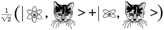
Figure 1: Cartoon representing Schrödinger’s cat paradox. (Reprinted from Physics Today by permission of the authors [19], and Physics Today.)

The cartoon shows a ket that presumably can be represented by a superposition of and not by an expansion in terms of two kets, one consisting of a radioactivity source and a live cat at an instant in time $t$, and the other a radioactivity source that has decayed at time $t+\tau$ and a dead cat that has been poisoned by the release of hydrocyanic acid induced by the radiation emitted at $t+\tau$.

The cartoon represents accurately Schrödinger’s cat paradox but corresponds to no physical reality because a ket is valid at a specific instant in time, and therefore cannot be represented by an expansion in terms of let alone superposition of two kets, one of which applies at time $t$, and the other at time $t+\tau$. Moreover, and for sure more importantly, a radioactivity source prior to decay is a system, that is, an entity both separable from and uncorrelated with its environment which includes a live cat and its life support interactions, such as breathing, drinking, eating, and (excuse the expression) other necessities of living beings. Solid and incontrovertible evidence for the physical realities just cited is provided by a very large number of radioactivity sources devoid of evil contraptions in hospitals, science and engineering laboratories, and nuclear energy installations, and a myriad of creatures, including human beings and cats, that live happily around these sources.

For clarity and avoidance of misinterpretations, at time $t$ the Hilbert space of the radioactivity source and the cat must be the direct product $\mathcal{H}_{{\rm r}1}\otimes\mathcal{H}_{{\rm lc}}$, and the catalog of probabilities by the direct product $\mbox{\Pifont{psy}r}_{{\rm r}1}\otimes\mbox{\Pifont{psy}r}{{}_{\rm lc}}$, where $\mathcal{H}_{\rm i}$ and $\mbox{\Pifont{psy}r}_{\rm i}$ for i=r1, lc are the Hilbert spaces and probability catalogs of the radioactivity source and the live cat, respectively. Most likely, even though not necessarily, the probability catalogs are density operators for both the radioactivity source and the live cat and not projectors or, equivalently, the entropy of each of these two systems is not zero. Moreover, each of the probability catalogs $\mbox{\Pifont{psy}r}_{{\rm r}1}$ and $\mbox{\Pifont{psy}r}_{{\rm lc}}$ is represented by a homogeneous or irreducible ensemble of identical systems, identically prepared (see A III and A V). It is clear that in the time interval $t$ to $t+\tau$ the quantum representation of the radioactivity source and the live cat does not involve a radioactivity source that has decayed and a dead cat.

At $t+\tau$, however, if radiation is emitted from the source and precipitates the poisoning and death of the cat, then we have an entirely new situation, that is, two new systems, two new entities each of which is separable from, and uncorrelated with its environment. The source is a system with fewer radioactive nuclei than were present at time $t$, and the cat is an entirely new system because a dead cat does not need to and does not interact with any life support systems, that is, the interaction between the radioactivity source and the live cat induces radical changes in both systems. At this time, the Hilbert space for the two systems is $\mathcal{H}_{{\rm r}2}\otimes\mathcal{H}_{{\rm dc}}$, and the probability catalog is $\mbox{\Pifont{psy}r}_{{\rm r}2}\otimes\mbox{\Pifont{psy}r}_{{\rm dc}}$, where the subscript r2 denotes the radioactivity source with fewer radioactive nuclei than at time $t$, and dc the dead cat. It is clear that both the new systems and the new probability catalogs have no part that refers to the source at time $t$ and a live cat. Said differently, no inference can be made about the radioactivity source prior to decay and the live cat by studying the radioactivity source after the decay and the dead cat because in each of the two intervals $t$ to $t+\tau$ and (time) $>t+\tau$ each of the two entities under consideration is both separable from and uncorrelated with its environment, that is, can be identified as a system.

After a discussion of theories of measurement, Schrödinger considers two systems that interact with each other for a certain time and then are separated. He says …

“This is the point. Whenever one has a complete expectation-catalog – a maximum total knowledge – a $\psi$-function for two completely separated bodies, or, in better terms, for each of them singly, then one obviously has it also for the two bodies together, i.e., if one imagines that neither of them singly but rather the two of them together make up the object of interest, of our questions about the future.”

“But the converse is not true. Maximal knowledge of a total system does not necessarily include total knowledge of all its parts, not even when these are fully separated from each other and at the moment are not influencing each other at all. Thus it may be that some part of what one knows may pertain to relations or stipulations between the two subsystems (we shall limit ourselves to two), as follows: if a particular measurement on the first system yields this result, then for a particular measurement on the second the valid expectation statistics are such and such; but if the measurement in question on the first system should have that result, then some other expectation holds for that on the second; should a third result occur for the first, then still another expectation applies to the second; and so on, in the manner of a complete disjunction of all possible measurement results which the one specifically contemplated measurement on the first system can yield. In this way, any measurement process at all or, what amounts to the same, any variable at all of the second system can be tied to the not-yet-known value of any variable at all of the first, and of course vice versa also. If that is the case, if such conditional statements occur in the combined catalog, then it can not possibly be the maximal in regard to the individual systems. For the content of two maximal individual catalogs would by itself suffice for a maximal combined catalog; the conditional statements could not be added on.”

“The insufficiency of the $\psi$-function as model replacement rests solely on the fact that one doesn’t always have it. If one does have it, then by all means let it serve as description of the state. But sometimes one does not have it, in cases where one might reasonably expect to. And in that case, one dare not postulate that it “is actually a particular one, one just doesn’t know it”; the above-chosen standpoint forbids this. “It” is namely a sum of knowledge; and knowledge that no ones knows, is none.”

“We continue. That a portion of the knowledge should float in the form of disjunctive conditional statements between the two systems can certainly not happen if we bring up the two from opposite ends of the world and juxtapose them without interaction. For then indeed the two “know” nothing about each other. A measurement on one cannot possibly furnish any grasp of what is to be expected of the other. Any “entanglement of predictions” that takes place can obviously only go back to the fact that the two bodies at some earlier time formed in a true sense one system, that is were interacting, and have left behind traces on each other. If two separated bodies, each by itself known maximally, enter a situation in which they influence each other, and separate again, then there occurs regularly that which I have just called “entanglement” of our knowledge of the two bodies. The combined expectation-catalog consists initially of a logical sum of the individual catalogs; during the process it develops causally in accord with known law (there is no question whatever of measurement here). The knowledge remains maximal, but at its end, if the two bodies have again separated, it is not again split into a logical sum of knowledges about the individual bodies. What still remains of that may have become less than maximal, even very strongly so. – One notes the great difference over against the classical model theory, where of course from known initial states and with known interaction the individual end states would be exactly known.”

Earlier we discuss most of the points raised in the preceding statements except for entanglement. In our terminology, entanglement means that no two systems can be defined after the interactions because the two parts may be separable from but correlated with each other (see Section 3.2.1 and A I).

We return to the issue of entanglement in Section 4 where we find that it is misinterpreted and misapplied.

3.2 Probability relations between separated systems

The title of this section is identical to the title of both communications that were presented on Schrödinger’s behalf at the Cambridge Philosophical Society by Born [5] and Dirac [6]. In both communications Schrödinger provides detailed mathematical relations that presumably describe what happens to two systems both before and after a temporary interaction.

3.2.1 Born communication

In the communication presented by Born [5] Schrödinger says:

“When two systems, of which we know the states by their respective representatives, enter into temporary physical interaction due to known forces between them, and when after a time of mutual influence the systems separate again, then they can no longer be described in the same way as before, viz. by endowing each of them with a representative of its own. I would not call that one but rather the characteristic trait of quantum mechanics, the one that enforces its entire departure from classical lines of thought. By the interaction the two representatives (or $\psi$-functions) have become entangled. To disentangle them we must gather further information by experiment, although we knew as much as anybody could possibly know about all that happened. Of either system, taken separately, all previous knowledge may be entirely lost, leaving us but one privilege; to restrict the experiments to one only of the two systems. After re-establishing one representative by observation, the other one can be inferred simultaneously. In what follows the whole of this procedure will be called the disentanglement. Its sinister importance is due to its being involved in every measuring process and therefore forming the basis of the quantum theory of measurement, threatening us thereby with at least a regressus in infinitum, since it will be noticed that the procedure itself involves measurement.”

As we discuss earlier, in quantum theory the definition of a system requires that it be separable from and uncorrelated with its environment (see A I). In principle, separability and lack of correlations are subject to experimental verification. For example, if the probabilities of the whole are found to be described by $\psi({\rm x}_{1},{\rm x}_{2})$, and the probabilities of the two parts by $\phi_{1}({\rm x}_{1})$ and $\phi_{2}({\rm x}_{2})$, respectively, then two systems are identifiable if and only if

$$\psi({\rm x}_{1},{\rm x}_{2})=\phi_{1}({\rm x}_{1})\phi_{2}({\rm x}_{2})$$

On the other hand, if the experimental results are such that

$$\psi({\rm x}_{1},{\rm x}_{2})\not=\phi_{1}({\rm x}_{1})\phi_{2}({\rm x}_{2})$$

then no two systems can be identified and, therefore, the two parts may be separable but entangled or correlated. Separability depends on the lack of forces between the constituents of the two systems, whereas lack of correlations depends on the lack of joint quantum probabilities between the constituents of the two systems.

Next, Schrödinger states:

“Attention has recently been called [2] to the obvious but very disconcerting fact that even though we restrict the disentangling measurements to one system, the representative obtained for the other system is by no means independent of the particular choice of observations which we select for that purpose and which by the way are entirely arbitrary. It is rather discomforting that the theory should allow a system to be steered or piloted into one or the other type of state at the experimenter’s mercy in spite of his having no access to it. This paper does not aim at a solution of the paradox, it rather adds to it, if possible. A hint as regards that presumed obstacle will be found at the end.”

In Sections 2.2 and 3.1 we show that there is neither an EPR nor a cat paradox. In particular, the cat paradox is disproven because it is based on the misconception that a probability catalog – projector or density operator – can be represented by an expansion in terms of (superposition of ?) two probability catalogs, each of which applies at a different instant in time, for example live cat and dead cat. Such a misconception is contrary to the structure of all non-relativistic paradigms of physics because in each of these paradigms the definitions of the concepts system, property, and state refer to one instant in time, and the evolution in time is accounted by the equation of motion of each paradigm.

The hint alluded to earlier states:

“The paradox would be shaken, though, if an observation did not relate to a definite moment. But this would make the present interpretation of quantum mechanics meaningless, because at present the objects of its predictions are considered to be the results of measurements for definite moments of time.”

The resolution suggested by the hint is not only contrary to the meaning of quantum measurements but more importantly it is detrimental to the most powerful characteristic of modern physics, namely, the equation of motion of each paradigm. The equation of motion allows scientists and engineers to make predictions, and, as such, builds into each paradigm the opportunity for its readjustment in case the predictions are not consistent with all future momentary perceptions. So the idea of considering more than one instant in time deprives physics of this wonderful flexibility of readjustment so as to include newer perceptions, and thus would tie each paradigm to preconceived faith rather than to experimental observations.

3.2.2 Dirac communication

In the introductory remarks of the Dirac communication [6], Schrödinger says:

“1. An earlier paper [5] dealt with the following fact. If for a system which consists of two entirely separated systems the representative (or wave function) is known, then the current interpretation of quantum mechanics obliges us to admit not only that by suitable measurements, taken on one of the two parts only, the state (or representative or wave function) of the other part can be determined without interfering with it, but also that, in spite of this non-interference, the state arrived at depends quite decidedly on what measurements one chooses to take – not only on the results they yield. So the experimenter, even with this indirect method, which avoids touching the system itself, controls its future state in very much the same way as is well known in the case of a direct measurement. In this paper it will be shown that the control, with the indirect measurement, is in general not only as complete but even more complete. For it will be shown that in general a sophisticated experimenter can, by a suitable device which does not involve measuring non-commuting variables, produce a non-vanishing probability of driving the system into any state he chooses; whereas with the ordinary direct method at least the states orthogonal to the original one are excluded.”

“The statement is hardly more than a corollary to a theorem about “mixtures” [7] for which I claim no priority but the permission of deducing it in the following section, for it is certainly not well known.”

“2. Supposing we knew that a system at a given moment were in either one or other of the sequence of states corresponding to the following sequence of wave functions $\psi_{i}$, finite or infinite in number, normalized but in general not orthogonal; supposing further we knew the probabilities of the system being in any one of these states – they must, of course, sum up to unity and shall be the real positive numbers $w_{i}$ written in the second line below the symbol of the function or state:

$$\left.\begin{array}[]{ccccc}\psi_{1}&\psi_{2}&\psi_{3}&\psi_{4}&...\\ w_{1}&w_{2}&w_{3}&w_{4}&...\\ (c^{\ast}_{1k})&(c^{\ast}_{2k})&(c^{\ast}_{3k})&(c^{\ast}_{4k})&...\end{array}\right\}.\hskip 144.54pt(1)$$

In the third line I have written the $k$th development coefficient of the function above, with respect to an arbitrary complete orthogonal system, chosen as a frame of reference to start with. The brackets are to indicate that the $k$th is meant as a representative of all of them; $(c^{\ast}_{3k})$, for instance, means all the development coefficients of $\phi_{3}$.”

“The mean value (or expectation value) of a physical variable $A$, represented in our frame of reference by the matrix $A_{lk}$, is

$$\bar{A} = w_{1}\sum_{l,k}c^{\prime\ast}_{1l}A_{1k}c^{\prime}_{1k}+w_{2}\sum_{l,k}c^{\prime\ast}_{2l}A_{lk}c^{\prime}_{2k}+...$$

$$= \sum_{l,k}A_{lk}\sum_{i}w_{i}c^{\prime}_{ik}c^{\prime\ast}_{il}.$$

Let us call $U$ the object, represented by the matrix whose $(k,l)$th element is

$$\hskip 144.54ptU_{kl}=\sum_{i}w_{i}c^{\prime}_{ik}c^{\prime\ast}_{il}\ ,\hskip 144.54pt(2)\\$$

then

$$\hskip 144.54pt\ \bar{A}=\ {\rm Trace}\ (AU).\hskip 144.54pt(3)$$

This trace (i.e. sum of diagonal terms) is obviously independent of the frame of reference, since the $w_{i}$ are, by their meaning, invariants and $U$ therefore transforms like a matrix representing a physical variable, e.g., like $A$.”

“Since the mean values are all that quantum mechanics predicts at all, the knowledge of $U$ in a definite frame of reference exhausts our real knowledge of the situation, just as in the case of a “state” the wave function exhausts it. The detailed times (1) from which $U_{kl}$ is composed may refer to the origin of our knowledge. But if another set of similar times leads to the same $U$, then it would be entirely meaningless to distinguish between the two physical situations. $U$ is von Neumann’s Statistical Operator. Its matrix is hermitian. It has the formal character of a real physical variable, but the physical meaning of a wave function, that is to say it describes the instantaneous physical situation of the system.”

”We propose to find all the different ways (or detailed data like (1)) which lead to the same U. Mark first, that the hermitian $U_{kl}$ is composed linearly, with positive coefficients $w_{i}$, whose sum total is unity, from matrices each of which obviously has the eigenvalues 1, 0, 0, 0, …, and therefore the trace 1. It follows that $U_{kl}$ has itself the trace 1 and non-negative eigenvalues. Now let us change the frame of reference by a canonical transformation, which makes $U$ diagonal. Let

$$\hskip 144.54ptp_{1},p_{2},p_{3},p_{4},...\hskip 144.54pt(4)$$

be this diagonal, the eigenvalues of $U$; according to what has just been said, they are non-negative and their sum is 1. This shows that the same mixture is obtained by mixing the orthogonal functions (or states) which form the basis of the new frame of reference, in the proportions (or with the probabilities) $p_{k}$.”

Earlier we review the question whether an experimenter, sophisticated or not, can determine the wave function of a system without performing direct measurements on it, and find a negative answer. We return to the issue here because of the association that Schrödinger makes between expectation values and a density operator $U$, defined as a statistical average of wave functions or projectors. To be sure, this is contrary to our proven result that density operators in quantum theory are defined exclusively by quantum mechanical probabilities, and not by quantum mechanical probabilities represented by projectors, and statistical probabilities of statistical theories of physics. However, Schrödinger’s discussion of $U$ contradicts his definition, and makes $U$ a density operator that is irreducible or unambiguous (see A V). Specifically, he emphasizes that “$U$ exhausts our real knowledge of the situation” and therefore that “there is no way of partitioning $U$ into a statistical average of projectors – wave functions”. Moreover, he asserts that “$U$ is determined by the only measurable quantities, that is the expectation values.” All these remarks are consistent with the exposition of quantum theory in the Appendix, and not with von Neumann’s statistical interpretation of density operators (see A XIV).

3.3 Summary of the comments on Schrödinger’s response to the EPR paper

Our summary about Schrödinger’s responses is to a large extend similar to the comments we made about the EPR paper. Three issues that need to be singled out here are the missed opportunity to recognize the importance of nonstatistical density operators, the suggested de-emphasis of the equation of motion as a predictor of events that have not yet been observed, and the incomplete characterization of entanglement.

4 Quantum Entanglement: A Modern Perspective

4.1 General Remarks

The title of this section is identical to the title of an article that appeared in Physics Today [19]. We discuss it here because it reflects several misconceptions that are present in many of the publications on quantum computation and quantum information. The authors of the article begin with brief discussions of the EPR paper and Schrödinger’s cat paradox, illustrated by the cartoon shown in Figure 1, and state;

“Erwin Schrödinger coined the word entanglement in 1935 in a three-part paper [3] on the “present situation in quantum mechanics.” His article was prompted by Albert Einstein, Boris Podolsky, and Nathan Rosen’s now celebrated EPR paper that had raised fundamental questions about quantum mechanics earlier that year. … For the three decades following the 1935 articles, the debate about entanglement and the “EPR dilemma” – how to make sense of the presumably nonlocal effect one particle’s measurement has on another – was philosophical in nature, and for many physicists it was nothing more than that. The 1964 publication by John Bell [20] changed that situation dramatically. Bell derived correlation inequalities that can be violated in quantum mechanics but have to be satisfied within every model that is local and complete — so-called local hidden-variable models. Bell’s work made it possible to test whether local hidden-variable models can account for observed physical phenomena. Early and ongoing recent experiments showing violations of such Bell inequalities have invalidated local hidden-variable models and lend support to the quantum-mechanical view of nature. In particular, an observed violation of a Bell inequality demonstrates the presence of entanglement in a quantum system.”

Earlier we show that there are no EPR and Schrödinger’s cat paradoxes. In addition we show that entanglement cannot occur in a system because, by definition, a system must be both separable from and uncorrelated with its environment (see A I). If both these conditions are not satisfied then no system can be defined. Moreover, entanglement is not related to hidden variables.

4.2 Entanglement for the 21st century

The authors of Ref. [19] say:

“An experimentalist, Alice, wishes to send an unknown state $|s\big{>}=\alpha|0\big{>}+\beta|1\big{>}$ of a two level quantum system to another experimentalist, Bob, in a distant laboratory. … Alice and Bob do not have the means of directly transmitting the quantum system from one place to another … but let us imagine that they do share an entangled state. Consider the case in which Alice and Bob each have one spin of a shared singlet state of two spin-1/2 particles $|\Psi^{-}\big{>}=1/\sqrt{2}(|\uparrow,\downarrow\big{>}+|\downarrow,\uparrow\big{>})$, also called EPR pair. Alice can transmit her spin $|s\big{>}$ to Bob by performing a certain joint measurement on her spin $|s\big{>}$ and her half of the EPR pair. She tells Bob the result of her measurement and depending on her information, Bob rotates his half of the EPR pair to obtain the state $|s\big{>}$.”

There are three statements in the preceding quote that we find contrary to quantum theory: (i) In principle, an infinite number of measurements on an ensemble of identical systems, identically prepared is needed to determine $|s\big{>}$, regardless of the values of $\alpha$ and $\beta$ $(\alpha^{2}+\beta^{2}=1)$. So how can one measurement reveal any information about $|s\big{>}$?; (ii) The ket $|\Psi^{-}\big{>}$ is not an EPR state. It is an expansion of $|\Psi^{-}\big{>}$ (not a superposition) in terms of two orthonormal eigenkets of a two-spin system; and (iii) a system is not a state, and a state is not a system.

Next, the authors of Ref. [19] say:

“The spin-singlet EPR state that Alice and Bob share in quantum teleportation is called a maximally entangled state. Even though the two spins together constitute a definite pure state, each spin state is maximally undetermined or mixed when considered separately. In mathematical terms, Alice’s local density matrix — obtained by tracing over Bob’s spin degrees of freedom, ${\rm Tr}_{B}(|\Psi^{-}\big{>}\big{<}\Psi^{-}|)$ — has equal probability for spin up and spin down. In keeping with Schrödinger’s understanding of entanglement, one measures the amount of entanglement in a general pure state $\phi$ in terms of the lack of information about its local parts. The von Neumann entropy $S(\mbox{\Pifont{psy}r})=-{\rm Tr}(\mbox{\Pifont{psy}r}{\rm log}\mbox{\Pifont{psy}r})$ is used as a measure of that information. In other words, the entropy of entanglement $E$ of the pure state $\phi$ is equal to the von Neumann entropy of, say, Alice’s density matrix $\mbox{\Pifont{psy}r}={\rm Tr}_{B}|\phi\big{>}\big{<}\phi|$.”

The statements just cited misrepresent the theory of quantum phenomena. The trace of any projector either $|\Psi^{-}\big{>}\big{<}\Psi^{-}|$ or $|\phi\big{>}\big{<}\phi|$ is equal to unity as can be readily and easily shown by finding the density matrix in a representation in a Hilbert space that has either $|\Psi^{-}\big{>}\big{<}\Psi^{-}|$ or $|\phi\big{>}\big{<}\phi|$ as one of its mutually orthogonal dimensions. Accordingly, the thermodynamic entropy of any projector is equal to zero. The von Neumann entropy is not relevant to this discussion, let alone the fact that it does not represent the entropy of thermodynamics (see A V).

4.3 Superpositions of versus expansions in terms of either kets or projectors

In many discussions of either quantum mechanics or quantum computation and quantum information, expressions of the forms

$$|\Psi\big{>}=\sum_{\rm i}a_{\rm i}|u_{\rm i}\big{>}~{}~{}{\rm or}~{}~{}\mbox{\Pifont{psy}r}=\sum_{\rm i}{\rm p}_{\rm i}|u_{\rm i}\big{>}\big{<}u_{\rm i}|$$

are interpreted as superpositions of $|u_{\rm i}\big{>}$’s or $|u_{\rm i}\big{>}\big{<}u_{\rm i}|$’s, respectively. For example, the ket $(|0\big{>}+|1\big{>})/\sqrt{2}$ is pictorially represented as shown in Figure 2 reproduced from Ref. [1]. Such a representation, however, is not correct because the ket just cited is not a superposition of two electronic levels or two spins of an atom but an expansion of the probability catalog of one spin in terms of two orthonormal kets of one spin. In general, any ket can be represented by an expansion in terms of a complete set of orthonormal eigenkets of an operator representing an observable, and of course, different expansions result for different orthonormal eigenkets. Similar remarks can be made about a density operator that is represented by a homogeneous or irreducible ensemble and various expansions in terms of complete sets of orthonormal eigenprojectors of various observables.

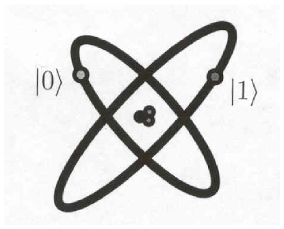
Figure 2: Qubit $(|0>+|1>)/\sqrt{2}$ represented by two electronic levels of an atom[1].

Nevertheless, the idea of superposition instead of expansion is so pervasive as to be considered a special feature of quantum theory. For example, Jozsa and Linden state [21]:

“One fundamental non-classical feature of the quantum formalism is the rule for how the space $S_{AB}$ of a composite system $AB$ is constructed from the state spaces $S_{A}$ and $S_{B}$ of the parts $A$ and $B$. In classical theory, $S_{AB}$ is the cartesian product of $S_{A}$ and $S_{B}$ whereas in quantum theory it is the tensor product (and the state spaces are linear spaces). This essential distinction between cartesian and tensor products is precisely the phenomenon of quantum entanglement viz. the existence of pure states of a composite system that are not product states of the parts.”

The statement just cited is not correct. First, the space in question is not the state space but the Hilbert space in which the probability catalogs (kets and/or density operators) are depicted. Second, as we discuss earlier, the tensor product is valid if and only if two systems can be identified, that is, if and only if two entities can be specified each of which is separable from and uncorrelated with its environment. If both requirements are not satisfied by the parts but are satisfied by their composite, then the composite is identified as a system, and entanglement has no meaning. Similar concerns about the meaning of the concept of entanglement are expressed by Wojcik [22].

Next, Jozsa and Linden state

“In quantum theory, state spaces always admit the superposition principle whereas in classical theory, state spaces generally do not have a linear structure. But there do exist classical state spaces with natural linear structure (e.g., the space of states of an elastic vibrating string with fixed end points) so the possibility of superposition in itself, is not a uniquely quantum feature.”

As we discuss earlier, this statement is not correct. Expansions of either kets or density operators are not superpositions, and cannot be visualized as “elastic vibrating strings with fixed endpoints.” In general, we feel very strongly that greater attention should be given to the use or abuse of the concept of entanglement because its correct consideration may disclose new approaches to the challenge of development of quantum computation and quantum information.

5 Conclusions

Upon detailed and close scrutiny of the ideas presented in the EPR paper and in Schrödinger’s responses to this paper, we find many faulty conclusions about the very successful theories of quantum mechanics and thermodynamics. We show that the faulty conclusions are due to lack of correct definitions of basic concepts, use of a postulate that is proven not to be valid, and misinterpretations of key theorems of the theory.

We also find that the faulty conclusions have permeated the theoretical underpinnings of quantum computation and quantum information. Our criteria are based on an exposition of quantum theory (see Appendix) that unifies quantum and thermodynamic ideas without resort to statistical probabilities.

We hope our review of the paradoxologies presented in both the EPR paper and in Schrödinger’s responses will be helpful in the development of a more rigorous approach to the fascinating and promising fields of quantum computation and quantum information.

Appendix: Quantum Theory

In this Appendix we present a summary of nonrelativistic quantum theory that differs from the presentations in most textbooks on the subject. The key differences are the discoveries that for a broad class of quantum-mechanical problems: (i) the probabilities associated with ensembles of measurement results at an instant in time require a mathematical concept delimited by but more general than a wave function or projector; and (ii) the evolution in time of the new mathematical concept requires an equation of motion delimited by but more general than the Schrödinger equation. Our definitions, postulates, and major theorems of quantum theory are based on slightly modified statements made by Park and Margenau [23], and close scrutiny of the implications of these statements.

The first difference is the recognition by Hatsopoulos and Gyftopoulos [8] that there exist two classes of quantum problems. In the first class, the quantum-mechanical probabilities associated with measurement results are fully described by wave functions or projectors, whereas in the second class the probabilities just cited require density operators that involve no statistical averaging over projectors — no mixtures of quantum and statistical probabilities. The same result emerges from the excellent review of the foundations of quantum mechanics by Jauch [9].

The second difference is the recognition that the evolution in time of non-statistical density operators requires a nonlinear equation of motion, and the discovery of such an equation by Beretta et al [24,25].

Kinematics: Definitions, postulates, and theorems at an instant in time.

A I: System. The term system means a set of specified types and amounts of constituents, confined and controlled by a nest of internal and external forces. For example, one hydrogen atom consisting of an electron and a proton confined in a three-dimensional cubical potential well of side size a. The internal force arises from the Coulomb interaction between the proton and the electron, and depends on the spatial coordinates of both constituents. The external force arises from the impermeable walls of the cubical box, that is, a force equal to infinity at every point on the inside surface of the cube. This force depends only on the spatial coordinates of either the electron or the proton or the hydrogen atom as a unit and not on any coordinates of constituents that are not included in the system, that is, the system is separable from its environment. In addition, in order to be totally independent and fully identifiable, the system must also be statistically uncorrelated with its environment. In general, this system definition is valid for any paradigm of physics, and sine qua non for quantum theory.

A II: System postulate. To every system there corresponds a complex, separate, complete, inner product space, a Hilbert space $\mathcal{H}$. The Hilbert space of a composite system of two distinguishable and identifiable subsystems 1 and 2, with associated Hilbert spaces $\mathcal{H}^{1}$ and $\mathcal{H}^{2}$, respectively, is the direct product space $\mathcal{H}^{1}\otimes\mathcal{H}^{2}$.

A III: Homogeneous or unambiguous ensemble. At an instant in time, an ensemble of identical systems is called homogeneous or unambiguous if and only if upon subdivision into subensembles in any conceivable way that does not perturb any member, each subensemble yields in every respect measurement results – spectra of values and frequency of occurrence of each value within a spectrum – identical to the corresponding results obtained from the ensemble. For example, the spectrum of energy measurement results and the frequency of occurrence of each energy measurement result obtained from any subensemble are identical to the spectrum of energy measurement results and the frequency of occurrence of each energy measurement result obtained from an independent ensemble that includes all the subensembles. Other criteria are presented in Ref. [8].

A IV: Preparation. A preparation is a reproducible scheme used to generate one or more homogeneous ensembles for study.

A V: Every textbook on quantum mechanics avers that the probabilities associated with measurement results of a system in a state “i” are described by a wave function $\Psi_{\rm i}$ or, equivalently, a projector $|\Psi_{\rm i}\big{>}\big{<}\Psi_{\rm i}|=\mbox{\Pifont{psy}r}_{\rm i}=\mbox{\Pifont{psy}r}_{\rm i}^{2}$ and that each density operator $\mbox{\Pifont{psy}r}>\mbox{\Pifont{psy}r}^{2}$ is a statistical average of projectors, that is, each psyr represents a mixture of quantum mechanical probabilities determined by projectors and nonquantum-mechanical or statistical probabilities that reflect our inability to make difficult calculations, our lack of interest in details, and our lack of knowledge of initial conditions. Mixtures have been introduced by von Neumann [7] for the purpose of explaining thermodynamic equilibrium phenomena in terms of statistical quantum mechanics (see also Jaynes [26] and Katz [27]).

Pictorially, we can visualize a projector by an ensemble of identical systems, identically prepared. Each member of such an ensemble is characterized by the same projector $\mbox{\Pifont{psy}r}_{\rm i}$, and von Neumann calls the ensemble homogeneous. Similarly, we can visualize a density operator psyr consisting of a statistical mixture of two projectors $\mbox{\Pifont{psy}r}=\alpha_{1}\mbox{\Pifont{psy}r}_{1}+\alpha_{2}\mbox{\Pifont{psy}r}_{2},\alpha_{1}+\alpha_{2}=1,\mbox{\Pifont{psy}r}_{1}\not=\mbox{\Pifont{psy}r}_{2}\not=\mbox{\Pifont{psy}r}$, where $\mbox{\Pifont{psy}r}_{1}$ and $\mbox{\Pifont{psy}r}_{2}$ represent quantum-mechanical probabilities, $\alpha_{1}$ and $\alpha_{2}$ represent statistical probabilities, and the ensemble is called heterogeneous or ambiguous [8]. A pictorial representation of a heterogeneous ensemble is shown in Figure A-1.

These results beg the questions (i) Are there quantum-mechanical problems that involve probability distributions which cannot be described by a projector but require a purely quantum-mechanical density operator — a density operator which is not a statistical mixture of projectors?; and (ii) Are such purely quantum-mechanical density operators consistent with the foundations of quantum mechanics?

HETEROGENEOUS ENSEMBLE
$\mbox{\Pifont{psy}r}_{1}$	$\mbox{\Pifont{psy}r}_{1}$	$\mbox{\Pifont{psy}r}_{1}$	$\cdots$	$\mbox{\Pifont{psy}r}_{2}$	$\mbox{\Pifont{psy}r}_{2}$
			$\mbox{\Pifont{psy}r}\neq\mbox{\Pifont{psy}r}_{1}$
$\mbox{\Pifont{psy}r}_{1}$	$\mbox{\Pifont{psy}r}_{1}$	$\mbox{\Pifont{psy}r}_{1}$	$\cdots$	$\mbox{\Pifont{psy}r}_{2}$	$\mbox{\Pifont{psy}r}_{2}$
			$\mbox{\Pifont{psy}r}\neq\mbox{\Pifont{psy}r}_{2}$
$\mbox{\Pifont{psy}r}_{1}$	$\mbox{\Pifont{psy}r}_{1}$	$\mbox{\Pifont{psy}r}_{1}$	$\cdots$	$\mbox{\Pifont{psy}r}_{2}$	$\mbox{\Pifont{psy}r}_{2}$
$\vdots$	$\vdots$	$\vdots$	$\cdots$	$\vdots$	$\vdots$
${\mbox{\footnotesize\sf FRACTION}}\ \mbox{\Pifont{psy}a}_{1}$				${\mbox{\footnotesize\sf FRACTION}}\ \mbox{\Pifont{psy}a}_{2}$
${\mbox{\footnotesize\sf OVERALL DENSITY}}\ \mbox{\Pifont{psy}r}=\mbox{\Pifont{psy}a}_{1}\mbox{\Pifont{psy}r}_{1}+\mbox{\Pifont{psy}a}_{2}\mbox{\Pifont{psy}r}_{2}$

Figure A-1: Pictorial representation of a heterogeneous ensemble. Each of the subensembles for $\mbox{\Pifont{psy}r}_{1}$ and $\mbox{\Pifont{psy}r}_{2}$ represents either a projector ($\mbox{\Pifont{psy}r}_{\mathrm{i}}=\mbox{\Pifont{psy}r}^{2}_{\mathrm{i}}$) or a density operator ($\mbox{\Pifont{psy}r}_{\mathrm{i}}>\mbox{\Pifont{psy}r}^{2}_{\mathrm{i}}$), for i = 1,2, and $\alpha_{1}+\alpha_{2}=1$

HOMOGENEOUS ENSEMBLE
psyr	psyr	psyr	$\cdots$	psyr
psyr	psyr	psyr	$\cdots$	psyr
psyr	psyr	psyr	$\cdots$	psyr
$\vdots$	$\vdots$	$\vdots$	$\cdots$	$\vdots$
${\mbox{\footnotesize\sf OVERALL DENSITY OPERATOR}}=\mbox{\Pifont{psy}r}$

Figure A-2: Pictorial representation of a homogeneous ensemble. Each of the members of the ensemble is characterized by the same density operator $\mbox{\Pifont{psy}r}\geq\mbox{\Pifont{psy}r}^{2}$. It is clear that any conceivable subensemble of a homogeneous ensemble is characterized by the same psyr as the ensemble.

Upon close scrutiny of the definitions, postulates, and key theorems of quantum theory, we find that the answers to both questions are yes. These answers were discovered by Hatsopoulos and Gyftopoulos [8] in the course of their development of a unified quantum theory of mechanics and thermodynamics, and by Jauch [9] in his systematic and rigorous analyses of the foundations of quantum mechanics (see also Section 3.2.2).

Pictorially, we can visualize a purely quantum-mechanical density operator $\mbox{\Pifont{psy}r}>\mbox{\Pifont{psy}r}^{2}$ by an ensemble of identical systems, identically prepared. Each member of such an ensemble is characterized by the same psyr as shown in Figure A-2; and by analogy to the results for a projector, we call this ensemble homogeneous or unambiguous [8]. If the density operator is a projector $\mbox{\Pifont{psy}r}_{\rm i}=\mbox{\Pifont{psy}r}_{\rm i}^{2}$, then each member of the ensemble is characterized by the same $\mbox{\Pifont{psy}r}_{\rm i}$ as originally proposed by von Neumann.

The recognition of the existence of density operators that correspond to homogeneous ensembles has many interesting implications. It extends quantum ideas to thermodynamics, and thermodynamic principles to quantum phenomena.

For example, it is shown that thermodynamics applies to all systems (both large and small, including one particle systems, such as one spin), to all states (both thermodynamic equilibrium, and not thermodynamic equilibrium), and that entropy is an intrinsic property of each constituent of a system [28] (in the same sense that inertial mass is a property of each constituent) and not a measure of ignorance, or lack of information, or disorder [29]. Again, it is shown that entropy is a measure of the quantum-mechanical spatial shapes of the constituents of a system, and that irreversibility is solely due to the changes of these shapes as the constituents try to conform to the external and internal force fields of the system [11,12]. Incidentally, for a spin, entropy is a measure of the orientation of the spin within or on the Block sphere (Figure A-3).

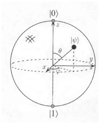
Figure A-3: Block sphere representation of a qubit.

It is noteworthy that for given values of energy, volume, and amounts of constituents, if psyr is a projector then the entropy $S$=0, if psyr is neither a projector nor a statistical average of projectors, and corresponds to a state which is not stable equilibrium (not thermodynamic equilibrium), then $S$ has a positive value smaller than the largest possible value for the given specifications, and if psyr corresponds to the unique stable equilibrium state, then $S$ has the largest value of all the entropies of the system which share the given values of energy, volume, and amounts of constituents. Said differently, all projectors or wave functions correspond to zero entropy physics, all largest entropy density operators for given system specifications correspond to stable equilibrium states – classical thermodynamics – and all other density operators that are associated neither with zero entropy, nor with largest value entropy correspond to probability distributions that can be represented neither by projectors nor by stable equilibrium state density operators. The few results just cited indicate that the restriction of quantum mechanics to problems that require probability distributions described only by projectors is both unwarranted and nonproductive.

A VI: Property. The term property refers to any attribute of a system that can be quantitatively evaluated at an instant in time by means of measurements and specified procedures. All measurement results and procedures are assumed to be precise, that is, both error free, and unaffected by the measurement and the measurement procedures. Moreover, they are assumed not to depend on either other systems or other instants in time.

A VII: Observable. From the definition just cited, it follows that each property can be observed. Traditionally, however, in quantum theory a property is called an observable only if it conforms to the following mathematical representations.

A VIII: Correspondence postulate. Some linear Hermitian operators A, B, … on Hilbert space $\mathcal{H}$, which have complete orthonormal sets of eigenvectors, correspond to observables of a system.

The inclusion of the word “some” in the correspondence postulate is very important because it indicates that there exist Hermitian operators that do not represent observables, and properties that cannot be represented by Hermitian operators. The first category accounts for Wick et al. [30] superselection rules, and the second accounts both for compatibility of simultaneous measurements introduced by Park and Margenau [23], and for properties, such as temperature, that are not represented by operators.

A IX: Measurement act. A measurement act is a reproducible scheme of measurements and operations on a member of an ensemble. Regardless of whether the measurement refers to an observable or not, in principle the result of such an act is presumed to be precise, that is, an error and perturbation free number.

If a measurement act of an observable is applied to each and every member of a homogeneous ensemble, the results conform to the following postulate and theorems.

A X: Mean-value postulate. If a measurement act of an observable represented by a Hermitian operator A is applied to each and every member of a homogeneous ensemble, there exists a linear functional m(A) of A such that the value of m(A) equals the arithmetic mean of the ensemble of A measurements, that is,

$${\rm m(A)}=\big{<}{\rm A}\big{>}=\sum_{\rm i}a_{\rm i}/{\rm N}\ ~{}{\rm for~{}N}\ \rightarrow\infty$$ (A-1)

where $a_{\rm i}$ is the measurement result of a measurement act of A applied to the ith member of the ensemble, a large number (theoretically infinite) of $a_{\rm i}$’s have the same numerical value, and both m(A) and $\big{<}$A$\big{>}$ represent the expectation value of A.

A XI: Mean-value theorem. For each of the mean-value functionals or expectation values m(A) of a system at an instant in time, there exists the same Hermitian operator psyr such that

$${\rm m(A)=}\big{<}{\rm A}\big{>}={\rm Tr}[\mbox{\Pifont{psy}r}{\rm A}]$$ (A-2)

The operator psyr is known as the density operator or the density of measurement results of observables, and here it can be represented solely by a homogeneous ensemble as shown in Figure A-2, that is, each member of the ensemble is characterized by the same psyr as any other member. It is noteworthy that the value $\big{<}$A$\big{>}$ of an observable A depends exclusively on the Hermitian operator A that represents the observable and on the density operator psyr, and not on any other operator that either commutes or does not commute with operator A.

The operator psyr is proven to be Hermitian, positive, unit trace and, in general, not a projector, that is,

$$\mbox{\Pifont{psy}r}>0;\ {\rm Tr}\mbox{\Pifont{psy}r}=1;\ {\rm and}\ \mbox{\Pifont{psy}r}\geq\mbox{\Pifont{psy}r}^{2}$$ (A-3)

A XII: Probability theorem. If a measurement act of an observable represented by operator A is applied to each and every member of a homogeneous ensemble characterized by psyr, the probability or frequency of occurrence $W(a_{\rm n})$ that the results will yield eigenvalue $a_{\rm n}$ is given by the relation

$$W(a_{\rm n})={\rm Tr}[\mbox{\Pifont{psy}r}{\rm A_{\rm n}}]$$ (A-4)

where A_n is the projection onto the subspace belonging to $a_{\rm n}$

$${\rm A}|\alpha_{\rm n}^{({\rm i})}>=a_{\rm n}|\alpha_{\rm n}^{({\rm i})}>\ \ \ {\rm for\ n}\ =1,2,...\ \ \ {\rm and\ i}\ =1,2,...,{\rm g}\ ,$$ (A-5)

and g is the degeneracy of $a_{\rm n}$.

A XIII: Measurement result theorem. The only possible result of a measurement act of the observable represented by A is one of the eigenvalues of A (Eq. A-5).

A XIV: State. The term state means all that can be said about a system at an instant in time, that is, a set of Hermitian operators A,B, … that correspond to a set of n²-1 linearly independent observables – the value of an independent observable can be varied without affecting the values of other observables – and the relations

$$\big{<}{\rm A}\big{>} = {\rm Tr}[\mbox{\Pifont{psy}r}{\rm A}]=\sum_{\rm i}a_{\rm i}/{\rm N}$$

$$\big{<}{\rm B}\big{>} = {\rm Tr}[\mbox{\Pifont{psy}r}{\rm B}]=\sum_{\rm i}b_{\rm i}/{\rm N}$$ (A-6)

$$\vdots \vdots \hskip 18.06749pt\vdots\hskip 18.06749pt\vdots\hskip 18.06749pt\vdots$$

where n is the dimensionality of the Hilbert space, and N $\rightarrow\infty$.

In Eqs. (A-6), either the density operator psyr is specified a priori and the values of the observables are calculated, or the values $\sum_{\rm i}a_{\rm i}/{\rm N}$, $\sum_{\rm i}b_{\rm i}/{\rm N},...$ of the linearly independent observables are either specified or, in principle, experimentally established and a unique operator psyr is calculated. The mappings both from psyr to expectation values and from expectation values to psyr are unique because Eqs. (A-6) are linear from expectation values to psyr and from psyr to expectation values.

It is noteworthy, that no quantum-theoretic requirement exists which excludes the possibility that the mapping from the measurable expectation values to psyr must yield a projector $\mbox{\Pifont{psy}r}=\mbox{\Pifont{psy}r}^{2}$ rather than a density operator $\mbox{\Pifont{psy}r}>\mbox{\Pifont{psy}r}^{2}$, and, conversely, that a pre-specified operator psyr must necessarily be a projector. In fact, the existence of density operators that are not derived as a mixture of quantum probabilities and statistical probabilities provides the means for the unification of quantum theory and thermodynamics without resorting to statistical considerations [8].

It is also noteworthy that only a linear operator X and its eigenvalues $x_{\rm i}$ are included in Eqs. (A-6). For example, only the Hamiltonian operator H and its eigenvalues $\epsilon_{1},\epsilon_{2},...,$ appear once in Eqs. (A-6). Operators H^m and their eigenvalues $\epsilon_{1}^{\rm m},\epsilon_{2}^{\rm m},...$ for m $>$ 1 are excluded. The reasons for this important restriction are: ($i$) For m even, information about the sign of eigenvalues of any X is lost; ($ii$) $\big{<}{\rm X}\big{>}$ and $\big{<}{\rm X^{m}}\big{>}$ for any m $>$ 1 are not linearly independent; and ($iii$) In general, in the extreme case that only X^m for m = 1, 2, … are used, then all the off-diagonal elements of psyr in the X representation are lost.

Finally, it is clear that the definition of state is not synonymous either with the concept of a wave function or the concept of a density operator (A XI). The definition of state requires both the specification of the system (A I), and either a complete set of measurable, linearly independent expectation values, or a prescribed density operator $\mbox{\Pifont{psy}r}\geq\mbox{\Pifont{psy}r}^{2}$ without any statistical probabilities.

A XV: Uncertainty relations. Ever since the inception of quantum mechanics, the uncertainty relation that corresponds to a pair of observables represented by non-commuting operators is interpreted by many scientists and engineers as a limitation on the accuracy with which the observables can be measured. For example, Heisenberg [31] writes the uncertainty relation between position $x$ and momentum $p_{x}$ in the form

$$\Delta x\Delta p_{x}\geq h$$ (A-7)

and comments: “This uncertainty relation specifies the limits within which the particle picture can be applied. Any use of the words “position” and “velocity” with an accuracy exceeding that given by equation (A-7) is just as meaningless as the use of words whose sense is not defined.”

Again Louisell [32] addresses the issue of uncertainty relations, and concludes: … “That is the actual measurement itself disturbs the system being measured in an uncontrollable way, regardless of the care, skill, or ingenuity of the experimenter. … In quantum mechanics the precise measurement of both coordinates and momenta is not possible even in principle.”

The remarks by Heisenberg and Louisell are representative of the intrepretations of uncertainty relations discussed in many textbooks on quantum mechanics [33]. These remarks, however, cannot be deduced from the postulates and theorems of quantum theory.

The measurement result theorem avers that the measurement of an observable is a precise (perturbation free) and, in many cases, precisely calculable eigenvalue of the operator that represents the observable. So neither a measurement perturbation nor a measurement error is contemplated by the theorem. An outstanding example of measurement accuracy is the Lamb shift [34].

The probability theorem avers that we cannot predict which precise eigenvalue each measurement will yield except in terms of either a prespecified or a measurable probability or frequency of occurrence.

It follows that an ensemble of measurements of an observable performed on an ensemble of identical systems, identically prepared yields a range of eigenvalues, and a probability or frequency of occurrence distribution over the eigenvalues. In principle, both results are precise and involve no disturbances induced by the measuring procedures.

To be sure, each probability distribution of an observable represented by operator X has a variance

$$\left(\Delta{\rm X}\right)^{2}={\rm Tr}\mbox{\Pifont{psy}r}{\rm X}^{2}-\left({\rm Tr}\mbox{\Pifont{psy}r}{\rm X}\right)^{2}=\big{<}{\rm X}^{2}\big{>}-\big{<}{\rm X}\big{>}^{2}$$ (A-8)

and a standard $\Delta{\rm X}$, where psyr is the projector or density operator that describes all the probability distributions of the problem in question. Moreover, for two observables represented by two non-commuting operators A and B, that is,

$${\rm AB}-{\rm BA}=i{\rm C}$$ (A-9)

it is readily shown that $\Delta{\rm A}$ and $\Delta{\rm B}$ satisfy the uncertainty relation [1,9,35]

$$\Delta{\rm A}\Delta{\rm B}\geq|\big{<}{\rm C}\big{>}|/2$$ (A-10)

It is evident that each uncertainty relation refers neither to any errors introduced by the measuring instruments nor to any particular value of a measurement result. The reason for the latter remark is that the value of an observable is determined by the expectation value of the operator representing the observable and not by any individual measurement result.

A XVI: Collapse of the wave function postulate. Among the postulates of quantum mechanics, many authoritative textbooks include von Neumann’s projection or collapse of the wave function postulate [33,36]. As we indicate earlier, an excellent, rigorous, and complete discussion of the falsity of the projection postulate is given by Park [16].

The only thing that we wish to add here is an argument against the postulate based on a violation of the position-momentum uncertainty relation. We consider a structureless particle confined in a one-dimensional, infinitely deep potential well of width $L$. Initially, the particle is in a state characterized by a projector $|\Psi\big{>}\big{<}\Psi|$. According to the projection postulate, upon a momentum measurement the particle must collapse into a momentum eigenstate. Suppose that the eigenstate just cited is characterized by the ith momentum projector $|{\rm p}_{\rm i}\big{>}\big{<}{\rm p}_{\rm i}|$. For such a projector, the standard deviation of position measurement results satisfies the relations $0<\Delta{\rm x}<L$, and the standard deviation of momentum measurement results $\Delta{\rm p}=0$. Accordingly, $\Delta{\rm x}\Delta{\rm p}=0<\hbar/2$ instead of $\Delta{\rm x}\Delta{\rm p}\geq\hbar/2.$ In view of the unquestionable validity of uncertainty relations, we must conclude that the projection postulate cannot be a valid postulate of quantum theory.

Dynamics: Evolution of the density operator in time

A XVII: Dynamical postulate. Hatsopoulos and Gyftopoulos [8] postulate that unitary transformations of psyr in time obey the relation

$${d\mbox{\Pifont{psy}r}\over dt}=-{i\over\hbar}\left[{\rm H}\mbox{\Pifont{psy}r}-\mbox{\Pifont{psy}r}{\rm H}\right]$$ (A-11)

where H is the Hamiltonian operator of the system. If H is independent of $t$, the unitary transformation of psyr satisfies the equation

$$\mbox{\Pifont{psy}r}(t)={\rm U}(t,t_{0})\mbox{\Pifont{psy}r}(t_{0}){\rm U}^{+}(t,t_{0})$$ (A-12)

where U⁺ is the Hermitian conjugate of U

$${\rm U}(t,t_{0})=\exp[-(i/\hbar)(t-t_{0}){\rm H}]$$ (A-13)

and if H is explicitly dependent on $t$

$${d{\rm U}\left(t,t_{0}\right)\over dt}=-\left(i/\hbar\right){\rm H}\left(t\right){\rm U}\left(t,t_{0}\right).$$ (A-14)

Though Eq. (A-11) is well known in the literature as the von Neumann equation, here it must be postulated for the following reason. In statistical quantum mechanics [37] the equation is derived as a statistical average of Schrödinger equations, each of which describes the evolution in time of a projector $\mbox{\Pifont{psy}r}_{\rm i}$ and each of which is multiplied by a time independent statistical probability $\alpha_{\rm i}$. But here, psyr is not a mixture of projectors and therefore cannot be derived as a statistical average of projectors. It is noteworthy that the dynamical postulate (Eq. A-11) is limited or incomplete because all unitary evolutions of psyr in time correspond to reversible adiabatic processes, but not all reversible adiabatic processes correspond to unitary evolutions of psyr in time [8] and not all processes are reversible.

A nonlinear equation of motion that describes both all reversible processes and all irreversible processes has been conceived by Beretta et al [24,25]. It is not discussed here for the sake of brevity. The only thing we wish to emphasize is that the Berettta equation is shown to satisfy all the requirements for it to be a bonafide equation of motion of a nonstatistical unified theory of quantum mechanics and thermodynamics [38].

References

1. M.A. Nielsen and I.L. Chuang, Quantum Computation and Quantum Information, Cambridge University Press, Cambridge, United Kingdom (2000).

2. A. Einstein, B. Podolsky, and N. Rosen, Phys. Rev., 47 777 (1935).

3. E. Schrödinger, Die Naturewissenschaften, 23 807; 823; 844 (1935).

4. E. Schrödinger, translation in English of Ref. [3], published in Proc. Amer. Phil. Soc., 124, 323 (1980).

5. E. Schrödinger, Proc. Cambridge Phil. Soc., 31, 555 (1935). Presented by Born.

6. E. Schrödinger, Proc. Cambridge, Phil. Soc., 446 (1936). Presented by Dirac.

7. J. von Neumann, Mathematical Foundations of Quantum Mechanics, Princeton University Press, NJ (1955).

8. G.N. Hatsopoulos, and E.P. Gyftopoulos, Found. of Physics, 6, 15; 6, 127; 6, 439; 6, 561 (1976).

9. J.M. Jauch, Foundations of Quantum Mechanics, Addison-Wesley, Reading, MA (1968).

10. T.S. Kuhn, The Structure of Scientific Revolutions, 2nd Edition, Chicago University Press, Chicago (1970).

11. E.P. Gyftopoulos, Int. J. Therm. Sci. 38 741 (1999).

12. E.P. Gyftopoulos, M.R. von Spakovsky, J. Energy Resources Tech. 125, 1 (2003).

13. H. Margenau, The Nature of Physical Reality, Oxbow Press, Woodbridge, Conn. (1977).

14. H. Margenau, Phys. Rev. 49 240 (1936).

15. H. Margenau, Phil. of Sci. 30, 6 (1963).

16. J.L. Park, Phil. of Sci. 35 3 (1968).

17. J.L. Park, AJP, 211 (1968).

18. R.C. Tolman, The Principles of Statistical Mechanics, Oxford University Press, Amen House, London (1962).

19. B.M. Terhal, M.M. Wolf, A.C. Doherty, Physics Today, April 2003, p. 46.

20. J.S. Bell, Physics 1, 195 (1964).

21. R. Josza, N. Linden, arXiv:quant-ph/0201143, v2, 8 Mar 2002.

22. A. Wójcik, Sci. 301, 5637, 1183 (2003).

23. J.L. Park, N. Margenau, Int. J. Theor. Phys., 1 211 (1968).

24. G.P. Beretta, E.P. Gyftopoulos, J.L. Park, and G.N. Hatsopoulos, Nuovo Cimento, 82B, 2, 169-191 (1984).

25. G.P. Beretta, E.P. Gyftopoulos, and J.L. Park, Nuovo Cimento, 87B, 1, 77-97 (1985).

26. E.T. Jaynes, Phys. Rev. 108(2) (1957).

27. A. Katz, Principles of Statistical Mechanics, The Information Theory Approach, W.H. Freeman and Company, San Francisco, CA (1967).

28. E.P. Gyftopoulos and E. Cubukcu, Phys. Rev. E, 55(4) (1997).

29. E.P. Gyftopoulos, J. Energy Res. and Tech., Trans ASME, 123 (2001).

30. G.C. Wick, A.S., Wightman, and E.P. Wigner, Phys. Rev. 88(1) (1952).

31. W. Heisenberg, The Principles of the Quantum Mechanics, translated into English by C. Eckart and F.C. Hoyt, Dover Publications (1930).

32. W.H. Louisell, Quantum Statistical Properties of Radiation, John Wiley & Sons, New York, NY (1973).

33. R. Shankar, Principles of Quantum Mechanics, Plenum Press, New York, NY (1994).

34. W.E. Lamb and R.C. Rutherford, Phys. Rev. 72(3) (1947).

35. D.J. Griffiths, Introduction to Quantum Mechanics, Prentice Hall, Englewood Cliffs, NJ (1994).

36. R.L. Liboff, Introductory Quantum Mechanics, Addison-Wesley, Reading, MA (1980).

37. R.C. Tolman, The Principles of Statistical Mechanics, Oxford University Press, Amen House, London (1962).

38. H.J. Korsh and H. Steffen, J. of Phys. A20, 3787 (1987).