Non-conditioned generation of Schrödinger cat states in a cavity

Abstract

We investigate the dynamics of a two-level atom in a cavity filled with a nonlinear medium. We show that the atom-field detuning $\delta$ and the nonlinear parameter $\chi^{(3)}$ may be combined to yield a periodic dynamics, allowing the generation of almost exact superpositions of coherent states (Schrödinger cats). By analysing the atomic inversion and the field purity, we verify that any initial atom-field state is recovered at each revival time, and that a coherent field interacting with an excited atom evolves to a superposition of coherent states at each collapse time. We show that a mixed field state (statistical mixture of two coherent states) evolves towards an almost pure pure field state as well (Schrödinger cat). We discuss the validity of those results by using the field fidelity and the Wigner function.

I Introduction

In quantum optics, the Jaynes-Cummings model (JCM) describes the interaction between a two-level atom and a single quantized mode of the radiation field in a lossless cavity and within the rotating wave approximation (RWA). The JCM is probably the simplest fundamental model of field-matter interaction with an exactly integrable Hamiltonian. Just over forty years since its introduction jay , the model has originated several studies in various contexts and with different purposes, and has become the basis for several generalizations and other models sho . More recently, important experimental achievements in cavity quantum electrodynamics (QED) and trapped ions have stimulated both theoretical and experimental research in that area mes . An interesting related subject is the quest for generation methods of macroscopically distinguishable superpositions of quantum states, or Schrödinger cat states tri . Several schemes using coherent states have been proposed yur ; gar ; guo ; dav ; pat , and a few experimental realizations have been already accomplished in cavity QED as well as in trapped ions systems bru ; bru2 ; mon . In cavity QED models, states close to those superpositions arise at specific times, for the cavity field initially in a coherent state gea or even in a statistical mixture of two coherent states fre . Propositions such as the Yurke-Stoler generation scheme yur , and those based on quantum non-demolition processes (QND), depend on very large values of Kerr nonlinearities, which is probably the main obstacle for their implementation bru . However, in the last few years, the observation of large Kerr nonlinearities with low intensity light ima ; reb ; kan as well as propositions involving small Kerr nonlinearities jeo have renewed the interest on those schemes. Furthermore, schemes for generation involving cavity QED with a nonlinear medium, based on atomic conditional measurements have also been proposed wei .

In this paper, we present a method that does not depend on conditional measurements. We have found that, the JCM with a nonlinear Kerr-like medium, under suitable combinations of the atom-field detuning $\delta$ and the nonlinear parameter $\chi^{(3)}$ and for an initial field prepared either in a coherent state or in a statistical mixture of two coherent states, makes possible a Schrödinger cat state generation with higher fidelity than the JCM without a nonlinear medium. We would like to remark that in the ordinary JCM, the initial field in a coherent state evolves to a state close to a Schrödinger cat state at a specific time, as reported in gea , and if we start with a statistical mixture of two coherent states, the field basically remains in a mixed state fre ; vid . The possibility of generating superpositions of coherent states in the JCM with a nonlinear Kerr-like medium with an atom-field detuning has not been yet addressed in the literature.

This paper is organized as follows: in section II we introduce the model and obtain the evolution operator in the RWA approximation. In section III we present the numerical results of some fundamental quantities and show how to obtain the condition for a periodic dynamics. In section IV, we discuss the main results and present our conclusions.

II Model

In this section we describe the interaction of a two-level atom with a high-Q single-mode cavity filled with a nonlinear Kerr-like medium, which can be modelled as an anharmonic oscillator aga . The cavity field is coupled with both the two-level atom and the nonlinear medium. If the response time of the nonlinear medium is sufficiently small we can adiabatically eliminate the photon-photon coupling, i.e. considering the field and nonlinear medium frequencies far from each other buz . Then, the total Hamiltonian of the system, with the adiabatic, RWA and dipole approximations, can be written as ban

$$\bm{H}=\hslash\omega_{0}\bm{a}^{\dagger}\bm{a}+\tfrac{1}{2}\hslash\omega_{eg}\bm{\sigma}_{\!z}+\hslash\chi^{(3)}\bm{a}^{\dagger}{}^{2}\bm{a}^{2}+\hslash\Omega(\bm{a}^{\dagger}\bm{\sigma}_{\!-}+\bm{a}\bm{\sigma}_{\!+}),$$ (1)

where $\omega_{0}$ ($\omega_{eg}$) is the cavity field (atomic transition) frequency, $\bm{a}^{\dagger}$ ($\bm{a}$) is the creation (annihilation) operator of the cavity mode obeying $[\bm{a},\bm{a}^{\dagger}]=\bm{1}$, $\bm{\sigma}_{\!z}=|e\rangle\langle{e}|-|g\rangle\langle{g}|$, $\bm{\sigma}_{\!+}=|e\rangle\langle{g}|$ and $\bm{\sigma}_{\!-}=|g\rangle\langle{e}|$ are the standard Pauli matrices operators, where $|e\rangle$ ($|g\rangle$) refer to the excited (ground) atom state, $\Omega$ is the atom-field coupling constant and $\chi^{(3)}$ is the nonlinear parameter, proportional to the dispersive part of the third-order nonlinear susceptibility jos .

Following the approach of Stenholm ste , we delineate the main steps to obtain the exact (under the RWA) time evolution operator for this model. After some algebra, we can rewrite equation (1) as

$$\bm{H}=\bm{H}_{0}+\bm{H}_{\rm int},$$ (2)

where

$$\bm{H}_{0}=\hslash\omega_{0}(\bm{a}^{\dagger}\bm{a}+\tfrac{1}{2}\bm{\sigma}_{\!z}),$$ (3a)

$$\bm{H}_{\rm int}=\bm{H}_{1}+\bm{H}_{2},$$ (3b)

with

$$\bm{H}_{1}=\tfrac{1}{2}\hslash\chi^{(3)}+\hslash\chi^{(3)}[(\bm{a}^{\dagger}\bm{a})^{2}+\bm{a}^{\dagger}\bm{a}\bm{\sigma}_{\!z}]-\hslash\chi^{(3)}(\bm{a}^{\dagger}\bm{a}+\tfrac{1}{2}\bm{\sigma}_{\!z}),$$ (4a)

$$\bm{H}_{2}=\hslash[\tfrac{\delta}{2}-\chi^{(3)}(\bm{a}^{\dagger}\bm{a}-\tfrac{1}{2})]\bm{\sigma}_{\!z}-\tfrac{1}{2}\hslash\chi^{(3)}+\hslash\Omega(\bm{a}^{\dagger}\bm{\sigma}_{\!-}+\bm{a}\bm{\sigma}_{\!+}),$$ (4b)

where $\delta=\omega_{eg}-\omega_{0}$ is the atom-field detuning.

We have verified that equation (3a) and equation (3b) commute, and, therefore we may write $\bm{H}_{I}=\bm{U}_{0}(t)\bm{H}_{\rm int}\bm{U}^{\dagger}_{0}(t)=\bm{H}_{\rm int}$, which is just the Hamiltonian in the interaction picture. Hence, the respective time evolution operator is given by

$$\bm{U}_{I}(t)=\bm{U}_{1}(t)\bm{U}_{2}(t)=\exp\left(-\dfrac{\imath}{\hslash}\bm{H}_{1}t\right)\exp\left(-\dfrac{\imath}{\hslash}\bm{H}_{2}t\right),$$ (5)

where the exponentials have been decoupled. After some manipulation we obtain the following form

$$\bm{U}_{I}(t)=\left(\begin{array}[]{ccc}\bm{E}_{n+1}&0\\ 0&\bm{E}_{n}\end{array}\right)\left(\begin{array}[]{ccc}\bm{A}_{n+1}&\bm{B}^{\dagger}_{n+1}\\ -\bm{B}_{n+1}&\bm{A}^{\dagger}_{n}\end{array}\right),$$ (10)

with

$$\bm{E}_{n+1}={\rm e}^{-\imath\chi^{(3)}\bm{n}^{2}t},$$ (11a)

$$\bm{A}_{n+1}=\cos{(\tfrac{1}{2}\bm{\Omega}_{n+1}t)}-\imath\bm{\gamma}_{n+1}\dfrac{\sin{(\tfrac{1}{2}\bm{\Omega}_{n+1}t)}}{\bm{\Omega}_{n+1}},$$ (11b)

$$\bm{B}_{n+1}=2\imath\Omega\bm{a}^{\dagger}\dfrac{\sin{(\tfrac{1}{2}\bm{\Omega}_{n+1}t)}}{\bm{\Omega}_{n+1}},$$ (11c)

where

$$\bm{\Omega}_{n+1}=\sqrt{\bm{\gamma}^{2}_{n+1}+4\Omega^{2}(\bm{n}+1)},$$ (12)

and $\bm{\gamma}_{n+1}=\delta-2\chi^{(3)}\bm{n}$.

The result in equation (12) has been already obtained, in another context xie .

III Atom-Field Dynamics

In what follows we are going to assume an uncorrelated initial atom-field state, i.e.

$$\bm{\rho}=\bm{\rho}_{\rm a}\otimes\bm{\rho}_{\rm f},$$ (13)

where $\bm{\rho}_{\rm a}$ is the initial atom density operator, initially an excited state $\bm{\rho}_{\rm a}=|e\rangle\langle{e}|$ and $\bm{\rho}_{\rm f}$ is the initial field density operator, initially either a coherent state $\bm{\rho}^{\rm cs}_{\rm f}=|\alpha\rangle\langle\alpha|$ or an equally weighted statistical mixture of two coherent states $\bm{\rho}^{\rm sm}_{\rm f}=\tfrac{1}{2}(|\alpha\rangle\langle\alpha|+|{-}\alpha\rangle\langle{-}\alpha|)$. In all cases $\alpha=|\alpha|{\rm e}^{\imath\phi}$, and we will fix $|\alpha|=\sqrt{\bar{n}}=5$. The general form of the initial field state in the Fock state basis is

$$\bm{\rho}_{\rm f}=\sum\limits_{n,m}\rho_{n,m}|n\rangle\langle{m}|,$$ (14)

where $\rho_{n,m}=\langle{n}|\bm{\rho}_{\rm f}|m\rangle$ are the initial field matrix elements. For the coherent state

$$\rho^{\rm cs}_{n,m}={\rm e}^{-|\alpha|^{2}}\dfrac{\alpha^{n}\alpha^{\ast}{}^{m}}{\sqrt{n!m!}},$$ (15)

and for the statistical mixture of two coherent states

$$\rho^{\rm sm}_{n,m}=\tfrac{1}{2}{\rm e}^{-|\alpha|^{2}}\dfrac{\alpha^{n}\alpha^{\ast}{}^{m}}{\sqrt{n!m!}}[1+(-1)^{n+m}].$$ (16)

Hence, the evolved atom-field state is given by

$$\bm{\rho}(t)=\bm{U}_{I}(t)\bm{\rho}\bm{U}^{\dagger}_{I}(t)=\left(\begin{array}[]{cc}\bm{\rho}_{ee}(t)&\bm{\rho}_{eg}(t)\\ \bm{\rho}_{ge}(t)&\bm{\rho}_{gg}(t)\end{array}\right),$$ (19)

whose elements in the atomic basis are

$$\bm{\rho}_{ee}(t)=\sum\limits_{n,m}\rho_{n,m}E_{n+1}E^{\ast}_{m+1}A_{n+1}A^{\ast}_{m+1}|n\rangle\langle{m}|,$$ (20a)

$$\bm{\rho}_{eg}(t)=-\sum\limits_{n,m}\rho_{n,m}E_{n+1}E^{\ast}_{m+1}A_{n+1}B^{\ast}_{m+1}|n\rangle\langle{m+1}|,$$ (20b)

$$\bm{\rho}_{ge}(t)=-\sum\limits_{n,m}\rho_{n,m}E_{n+1}E^{\ast}_{m+1}B_{n+1}A^{\ast}_{m+1}|n+1\rangle\langle{m}|,$$ (20c)

$$\bm{\rho}_{gg}(t)=\sum\limits_{n,m}\rho_{n,m}E_{n+1}E^{\ast}_{m+1}B_{n+1}B^{\ast}_{m+1}|n+1\rangle\langle{m+1}|,$$ (20d)

with

$$E_{n+1}={\rm e}^{-\imath\chi^{(3)}n^{2}t},$$ (21a)

$$A_{n+1}=\cos{(\tfrac{1}{2}\Omega_{n+1}t)}-\imath\gamma_{n+1}\dfrac{\sin{(\tfrac{1}{2}\Omega_{n+1}t)}}{\Omega_{n+1}},$$ (21b)

$$B_{n+1}=2\imath\Omega\sqrt{n+1}\dfrac{\sin{(\tfrac{1}{2}\Omega_{n+1}t)}}{\Omega_{n+1}},$$ (21c)

being

$$\Omega_{n+1}=\sqrt{\gamma^{2}_{n+1}+4\Omega^{2}(n+1)},$$ (22)

the generalized Rabi frequency, with $\gamma_{n+1}=\delta-2\chi^{(3)}n$.

Once that $\bm{\rho}(t)$ belongs to the trace class operators acting in the space corresponding to the direct product in equation (13) we can trace over the field variables in equation (19) to obtain the reduced atomic density operator

$$\bm{\rho}_{\rm a}(t)={\rm Tr}_{\rm f}[\bm{\rho}(t)]=\left(\begin{array}[]{lll}\lambda_{ee}&\lambda_{eg}\\ \lambda^{\ast}_{eg}&\lambda_{gg}\end{array}\right),$$ (25)

where $\lambda_{ij}=\sum\limits_{n}\langle{n}|\bm{\rho}_{ij}(t)|n\rangle$. Using equation (20), we have

$$\bm{\rho}_{\rm a}(t)=\sum\limits_{n}\rho_{n,n}|A_{n+1}|^{2}|e\rangle\langle{e}|+\sum\limits_{n}\rho_{n,n}|B_{n+1}|^{2}|g\rangle\langle{g}|$$

$$\hskip 27.00005pt-\sum\limits_{n}(\rho_{n+1,n}{\rm e}^{-\imath\chi^{(3)}(2n+1)t}A_{n+2}B^{\ast}_{n+1}|e\rangle\langle{g}|+{\rm c.c}).$$ (26)

Analogously, by tracing over the atomic variables, we obtain the (reduced) field density operator

$$\bm{\rho}_{\rm f}(t)={\rm Tr}_{\rm a}[\bm{\rho}(t)]=\sum\limits_{n,m}\rho_{n,m}(t)|n\rangle\langle{m}|,$$ (27)

where

$$\rho_{n,m}(t)=\langle{n}|\bm{\rho}_{\rm f}(t)|m\rangle=E_{n+1}E^{\ast}_{m+1}(\rho_{n,m}A_{n+1}A^{\ast}_{m+1}$$

$$+\>\rho_{n-1,m-1}{\rm e}^{2\imath\chi^{(3)}(n-m)t}B_{n}B^{\ast}_{m}),$$ (28)

are the evolved field matrix elements.

III.1 Atomic Inversion

A quantity usually measured in experimental cavity QED is the atomic population inversion bru3 ; pho , defined as the difference between the probabilities of finding the atom in the excited state and in the ground state. Here the atomic inversion is given by

$${\cal W}(t)={\rm Tr}_{\rm a}[\bm{\sigma}_{\!z}\bm{\rho}_{\rm a}(t)]=\sum\limits_{n}P_{n}(|A_{n+1}|^{2}-|B_{n+1}|^{2}),$$ (29)

where $P_{n}=\rho_{n,n}=\langle{n}|\bm{\rho}_{\rm f}|n\rangle$ is the initial field photon number distribution.

It is well known that the atomic inversion is very sensitive to the initial field photon number distribution $P_{n}$. For the field in the Fock state $\bm{\rho}^{\rm f}_{\rm f}=|n\rangle\langle{n}|$ we have $P^{\rm f}_{n}=\delta_{n,m}$, resulting a sinusoidal behaviour for ${\cal W}(t)$. If the initial field is the thermal state $\bm{\rho}^{\rm th}_{\rm f}=\sum\limits_{n}P^{\rm th}_{n}|n\rangle\langle{n}|$ we have $P^{\rm th}_{n}=\bar{n}^{n}/(\bar{n}+1)^{n+1}$, and a more irregular behaviour occurs pho . For the field states considered in this paper we have $P^{\rm cs}_{n}=P^{\rm sm}_{n}={\rm e}^{-|\alpha|^{2}}|\alpha|^{2n}/n!$ so that the atomic response, at least regarding the atomic inversion, is the same in either case. The atomic inversion reveals non-classical features: the Rabi frequency oscillations present collapses and revivals nar . We have parametrized the variable time as $t/t_{r}$ to allow a better comparison among the different plots in terms of the revival time $t_{r}$. In figure 1, we plot the atomic inversion as a function of $t/t_{r}$, having $\delta=\chi^{(3)}=0$, and we observe the pattern of oscillations characteristic of the ordinary JCM atomic dynamics.

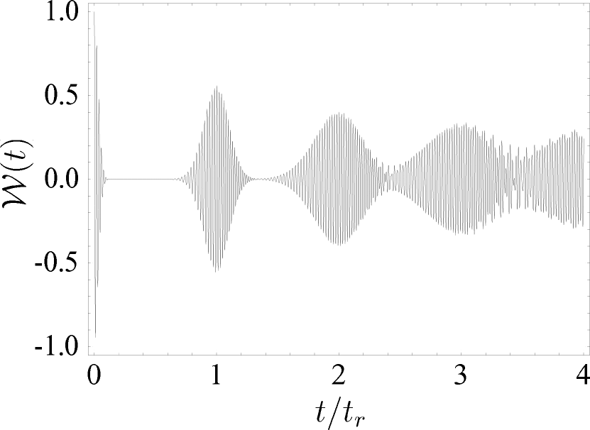
Figure 1: Atomic inversion as a function of $t/t_{r}$ when the field is initially in $\bm{\rho}^{\rm cs}_{\rm f}=|\alpha\rangle\langle\alpha|$ or $\bm{\rho}^{\rm sm}_{\rm f}=\frac{1}{2}(|\alpha\rangle\langle\alpha|+|{-}\alpha\rangle\langle{-}\alpha|)$ ($\alpha=5$, $\phi=0$) and the atom is initially in $\bm{\rho}_{\rm a}=|e\rangle\langle{e}|$ with $\delta=0$ and $\chi^{(3)}=0$.

III.2 Linear Rabi Frequency

We would like to find under which circumstances we may have a periodic dynamics. One way of doing that is to treat the Rabi frequency as a continuous quantity, so that we may expand equation (22) around the initial mean photon number $\bar{n}$

$$\Omega_{n+1}=\sum\limits_{k}\left.\dfrac{1}{k!}\dfrac{\partial^{k}\Omega_{n+1}}{\partial{n}^{k}}\right|_{n=\bar{n}}(n-\bar{n})^{k}.$$ (30)

The first term above governs the rapid oscillations in the Rabi frequency while the remaining terms generates the envelopes (revivals, super-revivals and so forth). It is well-know that two successive terms (in the discrete spectrum) of Rabi frequency, i.e. $\Omega_{\bar{n}+1}$ and $\Omega_{\bar{n}}$ have a $2\pi$ phase difference, so that the revival time is given by

$$t_{r}=2\pi\dot{\Omega}^{-1}_{n+1}\big{|}_{n=\bar{n}}=\pi\left|\dfrac{\Omega_{\bar{n}+1}}{\Delta_{\bar{n}+1}}\right|,$$ (31)

where $\Delta_{\bar{n}+1}=\Omega^{2}-\chi^{(3)}\gamma_{\bar{n}+1}$. If only the first two terms in equation (30) are nonzero, the Rabi frequency exhibits a perfectly periodic behaviour koz . This is the case, e.g. for the intensity-dependent JCM fre ; buc . We show that it also may be the case for the JCM with a Kerr-like medium: from the second order derivative of the Rabi frequency,

$$\ddot{\Omega}_{n+1}\big{|}_{n=\bar{n}}=4\left|\dfrac{\chi^{(3)}{}^{2}\Omega^{2}_{\bar{n}+1}-\Delta^{2}_{\bar{n}+1}}{\Omega^{3}_{\bar{n}+1}}\right|,$$ (32)

we have $\ddot{\Omega}_{\bar{n}+1}=0$ if $\Delta_{\bar{n}+1}=\chi^{(3)}\Omega_{\bar{n}+1}$ or equivalently

$$\delta_{c}=\dfrac{\Omega^{2}}{2\chi^{(3)}}-2\chi^{(3)},\qquad\mbox{(for all $n$)}.$$ (33)

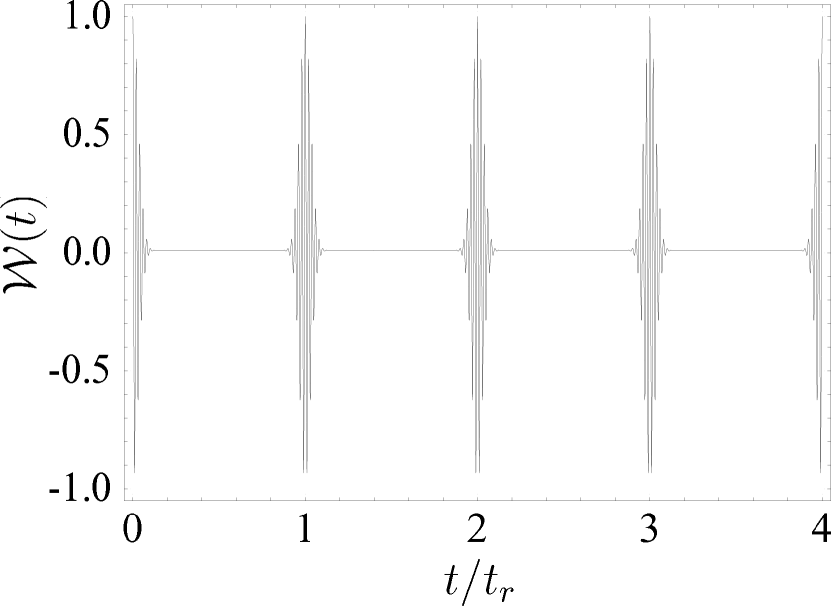
Figure 2: Atomic inversion as a function of $t/t_{r}$ when the field is initially in $\bm{\rho}^{\rm cs}_{\rm f}=|\alpha\rangle\langle\alpha|$ or $\bm{\rho}^{\rm sm}_{\rm f}=\frac{1}{2}(|\alpha\rangle\langle\alpha|+|{-}\alpha\rangle\langle{-}\alpha|)$ ($\alpha=5$, $\phi=0$) and the atom is initially in $\bm{\rho}_{\rm a}=|e\rangle\langle{e}|$ with $\delta=\delta_{c}=4.8\Omega$ and $\chi^{(3)}=0.1\Omega$.

It is clear from equation (30) that all higher-order derivatives up to the first-order vanish when $\delta=\delta_{c}$. This condition determines the periodic behaviour in the dynamics of the model. As a first illustration of that, we plot in figure 2, the atomic inversion for the same conditions of figure 1, but satisfying the relation for $\delta_{c}$ in equation (33) above which assures the periodic behaviour. Furthermore, if we insert equation (33) in equation (31), we obtain

$$t_{r}=\dfrac{\pi}{\chi^{(3)}},$$ (34)

and equation (22) becomes

$$\Omega_{n+1}=\delta_{c}+2\chi^{(3)}(n+2).$$ (35)

We remark that similar results were obtained, in another context, in the two-photon JCM with Kerr-like medium jos and in du , where the authors obtained the linearized Rabi frequency, although they just discussed the behaviour of the atomic inversion and used a strong-field approximation ($\bar{n}^{2}\gg\bar{n}$) to obtain the evolution operator.

We would like now to comment about the physical relevance of the values of $\delta$ taken in this paper, i.e. if they are consistent with the RWA. From experimental realizations in microwave cavity QED bru2 ; bru3 ; rem , we have that $\Omega\sim 10^{4}$Hz, $\omega_{eg}\sim 10^{6}$Hz, and $\omega_{0}\sim 10^{10}$Hz. Here we are considering $\delta\sim 10^{2}\Omega$Hz which is consistent with the RWA once that $\delta\sim 10^{-4}\omega_{0}\ll\omega_{0}$.

III.3 Field Purity

A very useful operational measure of the field state purity is given by the linear entropy

$$\zeta_{\rm f}(t)=1-{\rm Tr}_{\rm f}[\bm{\rho}^{2}_{\rm f}(t)]=1-\sum\limits_{n,m}|\rho_{n,m}(t)|^{2}.$$ (36)

In figure 3, we plot the linear entropy for the resonant case and in the absence of the Kerr-like medium, i.e. with $\chi^{(3)}=0$. It is well-known gea that at half of the revival time (collapse region), the initial coherent field evolves towards a field close to a pure (Schrödinger cat) state, figure 3-I, whereas for an initial statistical mixture of coherent states, the field is always far from a pure state vid , as shown in figure 3-II.

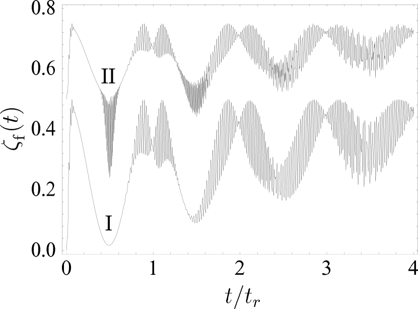
Figure 3: Field Purity as a function of $t/t_{r}$ when the field is initially in (I) $\bm{\rho}^{\rm cs}_{\rm f}=|\alpha\rangle\langle\alpha|$ or (II) $\bm{\rho}^{\rm sm}_{\rm f}=\frac{1}{2}(|\alpha\rangle\langle\alpha|+|{-}\alpha\rangle\langle{-}\alpha|)$ ($\alpha=5$, $\phi=0$) and the atom is initially in $\bm{\rho}_{\rm a}=|e\rangle\langle{e}|$ with $\delta=0$ and $\chi^{(3)}=0$.

The situation is very different if we consider the condition that gives a periodic dynamics. In figure 4 we plot the field purity for the same conditions as considered in the calculation of the atomic inversion. The initial coherent state evolves to an almost pure state (very close to a superposition of two coherent states, as we will discuss in what follows) at each collapse time and returns to the initial state at each revival time, figure 4-I. Remarkably, an initial statistical mixture of two coherent states also evolves to an almost pure state (approximately a superposition of two coherent states) at each collapse time and returns very close to the initial state at each revival time. As seen in the atomic inversion plot in figure 2, the initial atomic state is basically recovered at each revival time.

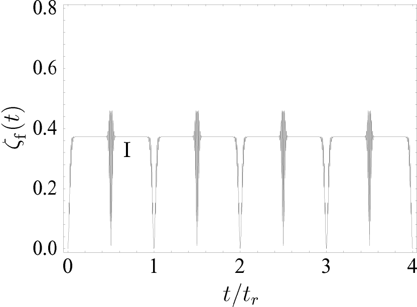
Figure 4: Linear entropy as a function of $t/t_{r}$ when the field is initially in (I) $\bm{\rho}^{\rm cs}_{\rm f}=|\alpha\rangle\langle\alpha|$ or (II) $\bm{\rho}^{\rm sm}_{\rm f}=\frac{1}{2}(|\alpha\rangle\langle\alpha|+|{-}\alpha\rangle\langle{-}\alpha|)$ ($\alpha=5$, $\phi=0$) and the atom is initially in $\bm{\rho}_{\rm a}=|e\rangle\langle{e}|$ with $\delta=\delta_{c}=4.8\Omega$ and $\chi^{(3)}=0.1\Omega$.

It is well known yur ; buz2 that a nonlinear Kerr-like medium may convert a field in a coherent state to another pure state, namely the Yurke-Stoler Schrödinger cat state. In the model present here, however, a field in an incoherent superposition (mixed mixture) can, under suitables conditions, evolve to a state very close to a pure state (a coherent superposition of two coherent states). In this case of course the other subsystem (atom) is left in a mixed state.

III.4 Q and Wigner Functions

In this subsection we consider the field dynamics from the point of view of the Q and the Wigner functions. The Q-function is a quasi-probability distribution which is the Fourier transform of the anti-normally ordered quantum characteristic function hil ; cah . For the field calculated here, the Q-function is given by

$$Q(\beta,t)=\dfrac{1}{\pi}\langle\beta|\bm{\rho}_{\rm f}(t)|\beta\rangle=\dfrac{1}{\pi}{\rm e}^{-|\beta|^{2}}\sum\limits_{n,m}\rho_{n,m}(t)\dfrac{\beta^{n}\beta^{\ast}{}^{m}}{\sqrt{n!m!}},$$ (37)

where $|\beta\rangle$ is a coherent state with $\beta=\Re(\beta)+\imath\Im(\beta)$.

In discussions found in the literature, the Q-function is plotted only at some specific times vid ; jos , as shown in figure 5. In order to provide more complete information about the field evolution, specially at the collapse time, when the pure state generation occurs, we present the full time evolution of the field Q-function as a form of an animation. The animation, external to this paper, can be downloaded from here. Interesting results arise when the dynamics is periodic: there is a relation between fractions of the revival time and the number of peaks in which the initial coherent field splits (or recombines), as shown in figure 5. For instance, at half-revival (collapse) time, the field becomes basically a pure (Schrödinger cat) state, represented by two peaks and an interference (oscillating) structure in phase-space. A similar behaviour occurs if the initial field is a statistical mixture of two coherent states: a pure Schrödinger cat state generation is almost perfect at half-revival time, although the initial state is a mixed state.

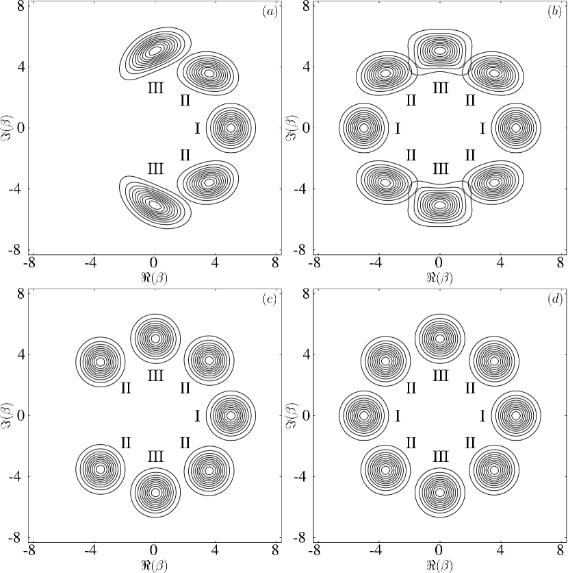
Figure 5: Q-function at (I) $t=0$, (II) $t=\frac{1}{4}t_{r}$, and (III) $t=\frac{1}{2}t_{r}$ when the field is initially in $(a,c)$ $\bm{\rho}^{\rm cs}_{\rm f}=|\alpha\rangle\langle\alpha|$ ($\alpha=5$, $\phi=0$) or $(b,d)$ $\bm{\rho}^{\rm sm}_{\rm f}=\frac{1}{2}(|\alpha\rangle\langle\alpha|+|{-}\alpha\rangle\langle{-}\alpha|)$ ($\alpha=5$, $\phi=0$) and the atom is initially in $\bm{\rho}_{\rm a}=|e\rangle\langle{e}|$ with $(a,b)$ $\delta=0$ and $\chi^{(3)}=0$ and $(c,d)$ $\delta=\delta_{c}=4.8\Omega$ and $\chi^{(3)}=0.1\Omega$.

For a better visualization of the field state generated at the collapse time we consider the Wigner function, a quasi-probability distribution given by the Fourier transform of the symmetrically ordered characteristic function cah . Alternatively it may be written as moy

$${}W(\beta,t)=\dfrac{2}{\pi}\displaystyle{\sum\limits_{n}}(-1)^{n}\langle{n},\beta|\bm{\rho}_{\rm f}(t)|n,\beta\rangle$$

$$=\dfrac{2}{\pi}\displaystyle{\sum\limits_{n,m}}(-1)^{n}\rho_{n,m}(t)\langle{m}|\bm{D}(2\beta)|n\rangle,$$ (38)

where $\bm{D}(2\beta)={\rm e}^{2(\beta\bm{a}^{\dagger}-\beta^{\ast}\bm{a})}$ is the Glauber displacement operator and

$$\langle{m}|\bm{D}(2\beta)|n\rangle=$$

$$\left\{\begin{array}[]{ll}{\rm e}^{-2|\beta|^{2}}\displaystyle{\sqrt{\frac{n!}{m!}}}(2\beta)^{m-n}L^{(m-n)}_{n}(4|\beta|^{2})&\quad(m\geqslant{n}),\\ {\rm e}^{-2|\beta|^{2}}\displaystyle{\sqrt{\frac{m!}{n!}}}(-2\beta^{\ast})^{n-m}L^{(n-m)}_{m}(4|\beta|^{2})&\quad(m\leqslant{n}),\end{array}\right.$$ (41)

where $L^{(n-m)}_{m}(4|\beta|^{2})$ are the associated Laguerre polynomials per .

In figure 6, we plot the Wigner function at the collapse time for the ordinary JCM, when the field is initially in the coherent state and the atom is initially excited. That corresponds to a state close to a Schrödinger cat state, in agreement with our field purity analysis, figure 3-I.

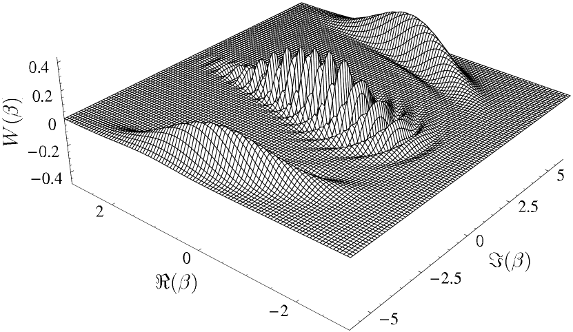
Figure 6: Wigner function at $t=\frac{1}{2}t_{r}$ when the field is initially in $\bm{\rho}^{\rm cs}_{\rm f}=|\alpha\rangle\langle\alpha|$ ($\alpha=5$, $\phi=0$) and the atom is initially in $\bm{\rho}_{\rm a}=|e\rangle\langle{e}|$ with $\delta=0$ and $\chi^{(3)}=0$.

When the condition for periodicity is fulfilled, the Wigner function at the corresponding time gives the state depicted in figure 7. We clearly see that the field is much closer to a Schrödinger cat state in this case. As we shall see, when the field is initially in a coherent state, all values of $\delta_{c}$ allow an almost Schrödinger cat state generation at each collapse time, with each cat state having a specific relative phase. For complementarity, we discuss in appendix A the situation of large detuning (dispersive approximation) based on an effective hamiltonian pei .

We would like to point out that the action of the Kerr-like medium itself is not enough to ‘purify’ the field. The Kerr-like medium merely converts the statistical mixture of two coherent states into another statistical mixture, as we show in appendix B. From the phase space point of view, the initial statistical mixture, figure 5-(b), splits in two deformed peaks, one for each coherent state of the incoherent superposition, in such a way that there is no perfect phase recombination at the collapse time. In the case of periodic dynamics, the peaks are uniform, as shown in figure 5-(d), and become virtually indistinguishable at the time they cross each other, which means that they correspond to an almost pure state.

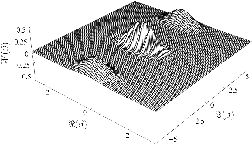
Figure 7: Wigner function at $t=\frac{1}{2}t_{r}$ when the field is initially in $\bm{\rho}^{\rm cs}_{\rm f}=|\alpha\rangle\langle\alpha|$ ($\alpha=5$, $\phi=0$) and the atom is initially in $\bm{\rho}_{\rm a}=|e\rangle\langle{e}|$ with $\delta=\delta_{c}=4.8\Omega$ and $\chi^{(3)}=0.1\Omega$.

III.5 Mean Photon Number

Now we present the procedure adopted to determine the relative phases of the superposition attained at each collapse time, depending on the values of $\delta$ and $\chi^{(3)}$ which satisfy equation (33). The first thing to note is that the mean photon number at the aaaaaaaaaaaaaaaaaaaaaaaaaaaaaaaaaaaaaaaaaaaaaaaaaaaaaaaaaaa

$\chi^{(3)}$	$0$	$0.5\Omega$	$0.4\Omega$	$0.3\Omega$	$0.2\Omega$	$0.10\bar{6}\Omega$	$0.1\Omega$	$0.05\Omega$	$0.01\Omega$	$0.005\Omega$
$\delta$	$0$	$0$	$0.45\Omega$	$1.0\bar{6}\Omega$	$2.1\Omega$	$4.4741\bar{6}\Omega$	$4.8\Omega$	$9.9\Omega$	$49.98\Omega$	$99.99\Omega$
$\bar{n}(\tfrac{1}{2}t_{r})$	$25.500$	$25.074$	$25.110$	$25.179$	$25.316$	$25.493$	$25.495$	$25.324$	$25.020$	$25.005$

Table 1: Mean photon number at $t=\tfrac{1}{2}t_{r}$ when the field is initially in $\bm{\rho}^{\rm cs}_{\rm f}=|\alpha\rangle\langle\alpha|$ or $\bm{\rho}^{\rm sm}_{\rm f}=\frac{1}{2}(|\alpha\rangle\langle\alpha|+|{-}\alpha\rangle\langle{-}\alpha|)$ ($\alpha=5$, $\phi=0$) and the atom is initially in $\bm{\rho}_{\rm a}=|e\rangle\langle{e}|$ for different values of $\delta$ and $\chi^{(3)}$.

collapse time may not be the same as the initial one.

To verify this we consider the mean photon number given by

$$\bar{n}(t)={\rm Tr}_{\rm f}[\bm{\rho}_{\rm f}(t)\bm{n}]=\sum\limits_{n}P_{n}(t)n,$$ (42)

where $P_{n}(t)$, for the model presented here, is given by

$$P_{n}(t)=\rho_{n,n}(t)=\langle{n}|\bm{\rho}_{\rm f}(t)|n\rangle=P_{n}|A_{n+1}|^{2}+P_{n-1}|B_{n}|^{2}.$$ (43)

As shown in table 1, for each combination of $\delta$ and $\chi^{(3)}$ we have a specific mean photon number at the collapse time.

III.6 Field Fidelity

To obtain the values of the relative phase $\vartheta$, of the superposition attained at the collapse time, we calculate the field fidelity, defined as

$${\cal F}_{\rm f}(t)={\rm Tr}_{\rm f}[\bm{\rho}_{\rm f}\bm{\rho}_{\rm f}(t)]=\sum\limits_{n,m}\rho_{m,n}\rho_{n,m}(t),$$ (44)

so that the evolved field state equals the initial field state if and only if ${\cal F}_{\rm f}(t)=1$. For that, we compare the field state obtained at $t=\tfrac{1}{2}t_{r}$, when the condition for the periodic dynamics is satisfied, to the following (Schrödinger cat) state

$$|\widetilde{\alpha};\vartheta\rangle={\cal C}^{\frac{1}{2}}(|\widetilde{\alpha}\rangle+{\rm e}^{\imath\vartheta}|{-}\widetilde{\alpha}\rangle),$$ (45)

i.e. $\bm{\rho}_{\rm f}=\bm{\rho}^{\rm cat}_{\rm f}=|\widetilde{\alpha};\vartheta\rangle\langle\widetilde{\alpha};\vartheta|$, where ${\cal C}=\tfrac{1}{2}(1+{\rm e}^{-2|\widetilde{\alpha}|^{2}}\cos{\vartheta})^{-1}$ is the normalization constant. From the mean photon number values at the collapse time we have $|\widetilde{\alpha}|^{2}=\bar{n}(\frac{1}{2}t_{r})$ with $\widetilde{\alpha}=|\widetilde{\alpha}|{\rm e}^{\imath\widetilde{\phi}}$, where the value $\widetilde{\phi}=\pi/2$ was obtained from the previous analysis of the Q-function (see figure 5). We then vary the values of the phase $\vartheta$ at the collapse time until we obtain ${\cal F}_{\rm f}(t)\approx 1$. The results are presented in table 2 for the initial coherent field state and the atom excited for different values of $\delta$ and $\chi^{(3)}$. Apart from the first combination (ordinary JCM), all the others satisfy equation (33) and we have the generation of a state very close to a Schrödinger cat state at each collapse time with a specific relative phase $\vartheta$. We have also found that, for an initial coherent field state with $\phi=\pi$, i.e. $\bm{\rho}^{\rm cs}_{\rm f}=|{-}\alpha\rangle\langle{-}\alpha|$, the relative phase of the generated superposition is given by $-\vartheta$, instead. We have payed special attention to the combinations (i) $\delta=4.8\Omega$ and $\chi^{(3)}=0.1\Omega$, which generates a state very close to an even coherent state ($\vartheta=0$), and (ii) $\delta=4.4741\bar{6}\Omega$ and $\chi^{(3)}=0.10\bar{6}\Omega$, aaaaaaaaaaaaaaaaaaaaaaaaaaaaaaaaaaaaaaaaaaaaaaaaaaaaaaaaaaa

$\chi^{(3)}$	$0$	$0.5\Omega$	$0.4\Omega$	$0.3\Omega$	$0.2\Omega$	$0.10\bar{6}\Omega$	$0.1\Omega$	$0.05\Omega$	$0.01\Omega$	$0.005\Omega$
$\delta$	$0$	$0$	$0.45\Omega$	$1.0\bar{6}\Omega$	$2.1\Omega$	$4.4741\bar{6}\Omega$	$4.8\Omega$	$9.9\Omega$	$49.98\Omega$	$99.99\Omega$
$\vartheta$	$1.21\pi$	$0.45\pi$	$0.52\pi$	$0.4\pi$	$0.7\pi$	$\pi$	$0$	$1.23\pi$	$1.49\pi$	$1.5\pi$
${\cal F}_{\rm f}(\tfrac{1}{2}t_{r})$	$0.7872$	$0.9674$	$0.9418$	$0.9231$	$0.8751$	$0.9883$	$0.9924$	$0.9318$	$0.9897$	$0.9973$

Table 2: Field fidelity at $t=\tfrac{1}{2}t_{r}$ for the field initially in $\bm{\rho}^{\rm cs}_{\rm f}=|\alpha\rangle\langle\alpha|$ ($\alpha=5$, $\phi=0$) and atom initially in $\bm{\rho}_{\rm a}=|e\rangle\langle{e}|$ for different values of $\delta$ and $\chi^{(3)}$ with the respective relative phase $\vartheta$.

which generates a state very close to an odd coherent state ($\vartheta=\pi$): those combinations are the only ones that enable the generation of an almost Schrödinger cat state at each collapse time when the initial field state is either a coherent state or a statistical mixture of two coherent states. In appendix B we (analytically) show how such results could be understood.

IV Conclusions

In this work we have investigated the dynamics of a field in a lossless cavity interacting with a two-level atom in the presence of a nonlinear Kerr-like medium. Using the density operator formalism, we have obtained the exact (RWA) evolution operator for this model. We have found that the dynamics of the JCM with a Kerr-like medium is considerably richer than shown in the literature. The parameters $\delta$ and $\chi^{(3)}$ may combine in a way that new and interesting features are revealed: for instance, we may obtain a periodic dynamics, contrarily to what happens in the ordinary JCM.

The field interacting just with a two-level atom evolves to a state not that close to a Schrödinger cat. On the other hand, a Kerr-like medium alone may split a single coherent state into a superposition of two coherent states, but a very large nonlinearity is required for that. In any case the generation of pure states from a mixed state is not verified. In our model both a Kerr-like medium and an atom conveniently detuned from the field are important in the nonclassical field generation process. The fine tuning of $\delta$ is important if one wants to match a specific value of the nonlinear parameter $\chi^{(3)}$, in order to achieve a periodic dynamics. Particularly, with a finite detuning there is no need of large Kerr nonlinearities, given that in a certain range of parameters, the larger the detuning the smaller the nonlinearity required. However, the detuning does not play a critical role in the generation scheme, because even for a zero detuning we have a value for the nonlinear parameter (large, though) that gives us a periodic dynamics. Although schemes based on non-resonant (large detuning) interactions do not require precise control over the detuning, they normally rely upon conditioned measurements. In particular, we observed that the periodic dynamics, dictated by $\delta_{c}$, allows us to recover the initial state at each revival time. We have also found that an initially coherent field becomes an almost exact superposition of coherent states (Schrödinger cat state) at each collapse time. The advantage of our method is that generation of sharp Schrödinger cat-like states of the field may be achieved in a non-conditioned manner, i.e. without the need of collapsing the atomic state. It seems that the non-linearity of a Kerr-like medium has an effect on the field that closely resembles the non-linear behaviour resulting from an atomic measurement, in the case of a conditional method.

We have also found the conditions in which a field initially in a statistical mixture of two coherent states evolves towards an almost pure state, e.g. close to an even coherent state. Such a quantum field ‘purification’ may be well understood from the phase space point of view: as the field undergoes periodic evolution, at certain times the overlap of Q-functions coming from opposite branches is almost perfect, meaning that an almost pure state (Schrödinger cat) has been generated. In order to better illustrate the field state generation process, we have calculated the cavity field Q-function for successive (close enough) times in a way that we could produce an animation of the complete evolution of the Q-function from $t=0$ until half of the revival time. The generation of an almost pure field state from a mixed state may of course be achieved at the expense of the purity of the atomic states, i.e. the atom itself ends up in a mixed state.

Appendix A Analytical results for the dispersive limit

We consider here the usual procedure to obtain the dispersive Hamiltonian for the JCM pei , but including a Kerr-like medium. The dressed states maintain their usual form

$$|+,n\rangle=\sin\theta_{n+1}|e,n\rangle+\cos\theta_{n+1}|g,n+1\rangle,$$ (46a)

$$|-,n\rangle={-}\cos\theta_{n+1}|e,n\rangle+\sin\theta_{n+1}|g,n+1\rangle,$$ (46b)

but the coefficients are given by

$$\sin\theta_{n+1}=\dfrac{\omega_{n+1}}{\sqrt{{(\Omega_{n+1}-\gamma_{n+1})}^{2}+{\omega^{2}_{n+1}}}},$$ (47a)

$$\cos\theta_{n+1}=\dfrac{(\Omega_{n+1}-\gamma_{n+1})}{\sqrt{{(\Omega_{n+1}-\gamma_{n+1})}^{2}+{\omega^{2}_{n+1}}}},$$ (47b)

where $\omega_{n+1}=2\Omega\sqrt{n+1}$. The corresponding eigenvalues are

$$E_{\pm,n}=\hslash\omega_{0}(n+\tfrac{1}{2})+\hslash\chi^{(3)}n^{2}\pm\tfrac{1}{2}\hslash\Omega_{n+1}.$$ (48)

The dispersive limit is obtained when we consider $\bm{H}_{\rm int}$, equation (3b), as a small perturbation of the whole Hamiltonian pei . It is equivalent to make

$$|\delta|\gg\omega_{n+1},$$ (49)

for any ‘relevant’ $n$. Under that condition, equation (48) becomes

$$E_{\pm,n}\approx\hslash\omega_{0}(n+\tfrac{1}{2})\pm\tfrac{1}{2}\hslash|\delta|+\hslash\chi^{(3)}n(n\mp 1)\pm\dfrac{\hslash\Omega^{2}}{|\delta|}(n+1),$$ (50)

meaning that we can employ the following effective Hamiltonian

$$\bm{H}^{\rm eff}=\hslash\omega_{0}\bm{a}^{\dagger}\bm{a}+\tfrac{1}{2}\hslash\omega_{eg}\bm{\sigma}_{\!z}+\hslash\chi^{(3)}\bm{a}^{\dagger}{}^{2}\bm{a}^{2}$$

$$+\>\dfrac{\hslash\Omega^{2}}{\delta}(\bm{a}^{\dagger}\bm{a}\bm{\sigma}_{\!z}+\bm{\sigma}_{\!+}\bm{\sigma}_{\!-}).$$ (51)

Analogously to the calculation of section II, we have the evolution operator for the dispersive limit given by

$$\bm{U}^{\rm eff}_{I}(t)={\rm e}^{-\imath\chi^{(3)}(\bm{n}^{2}-\bm{n})t}\left(\begin{array}[]{cc}{\rm e}^{-\imath\frac{\Omega^{2}}{\delta}(\bm{n}+1)t}&0\\ 0&{\rm e}^{\imath\frac{\Omega^{2}}{\delta}\bm{n}t}\end{array}\right),$$ (54)

so that we may write the evolved field state as

$$|\psi_{\rm f}(t)\rangle=\sum\limits_{n}c_{n}{\rm e}^{-\imath\chi^{(3)}n^{2}t}{\rm e}^{\imath\chi^{(3)}nt}{\rm e}^{-\imath\frac{\Omega^{2}}{\delta}nt}|n\rangle,$$ (55)

where $c_{n}=\exp(-|\alpha|^{2}/2)\alpha^{n}/\sqrt{n!}$ is the coherent state coefficient in the number state basis. We are now able to demonstrate the initial field state being recovered at each revival time and the generation of a Schrödinger cat state at each collapse time:

Case 1: When $\delta=\delta_{c}$, e.g. $\delta=49.98\Omega$ and $\chi^{(3)}=0.01\Omega$, we recover the initial state at $t_{r}=\pi/\chi^{(3)}$

$$|\psi_{\rm f}(t_{r})\rangle={\rm e}^{-\frac{1}{2}|\alpha|^{2}}\sum\limits_{n}\dfrac{1}{\sqrt{n!}}({\rm e}^{-\imath\pi\frac{\Omega^{2}}{\delta\chi^{(3)}}}\alpha)^{n}|n\rangle\approx|\alpha\rangle.$$ (56)

We remark that this result can be easily generalized for any initial field state.

Case 2: Similarly, at $\tfrac{1}{2}t_{r}=\pi/2\chi^{(3)}$ the field evolves to

$$|\psi_{\rm f}({\tfrac{1}{2}}t_{r})\rangle={\rm e}^{-\frac{1}{2}|\alpha|^{2}}\sum\limits_{n}\dfrac{1}{\sqrt{n!}}(\imath\alpha)^{n}{\rm e}^{-\imath\frac{\pi}{2}{n}^{2}}|n\rangle.$$ (57)

If we use ${\rm e}^{-\imath\frac{\pi}{2}n^{2}}=\tfrac{1}{2}(1+\imath)({\rm e}^{-\imath\pi{n}}-\imath)$, after multiplying by $\tfrac{1}{\sqrt{2}}(1-\imath)$, we obtain

$$|\psi_{\rm f}(\tfrac{1}{2}t_{r})\rangle=\dfrac{1}{\sqrt{2}}(|{-}\imath{\rm e}^{-\imath\frac{\pi}{2}\frac{\Omega^{2}}{\delta\chi^{(3)}}}\alpha\rangle-\imath|\imath{\rm e}^{-\imath\frac{\pi}{2}\frac{\Omega^{2}}{\delta\chi^{(3)}}}\alpha\rangle)$$

$$=\dfrac{1}{\sqrt{2}}(|\imath\alpha\rangle-\imath|{-}\imath\alpha\rangle),$$ (58)

in agreement to the numerical result ${\rm e}^{\imath\vartheta}={\rm e}^{\imath 1.49\pi}\approx{-}\imath$.

Appendix B From a statistical mixture to the Schrödinger cat

In the numerical analysis we have noted that the field initially in a coherent state with $\phi=0$ evolves to a Schrödinger cat with $\vartheta$ and the field initially in a coherent state with $\phi=\pi$ evolves to a Schrödinger cat with $-\vartheta$. Therefore, it is reasonable to suppose that the field initially prepared in a statistical mixture of those two coherent states evolves to the state

$$\bm{\rho}^{\rm sm\,cat}_{\rm f}=\tfrac{1}{2}(|\widetilde{\alpha};\vartheta\rangle\langle\widetilde{\alpha};\vartheta|+|\widetilde{\alpha};{-}\vartheta\rangle\langle\widetilde{\alpha};{-}\vartheta|),$$ (59)

i.e. a statistical mixture of two Schrödinger cat states with the same relative phase except for a minus sign. Finally, the reason why only even and odd coherent states are obtained during the evolution of an initial statistical mixture of two coherent states becomes clear by noting that

$$\bm{\rho}^{\rm cat}_{\rm f}=|\widetilde{\alpha};\vartheta\rangle\langle\widetilde{\alpha};\vartheta|={\cal C}[|\widetilde{\alpha}\rangle\langle\widetilde{\alpha}|+|{-}\widetilde{\alpha}\rangle\langle{-}\widetilde{\alpha}|$$

$$+\>\cos{\vartheta}(|\widetilde{\alpha}\rangle\langle{-}\widetilde{\alpha}|+|{-}\widetilde{\alpha}\rangle\langle\widetilde{\alpha}|)-\imath\sin{\vartheta}(|\widetilde{\alpha}\rangle\langle{-}\widetilde{\alpha}|-|{-}\widetilde{\alpha}\rangle\langle\widetilde{\alpha}|)],$$ (60)

and

$$\bm{\rho}^{\rm sm\,cat}_{\rm f}=\tfrac{1}{2}(|\widetilde{\alpha};\vartheta\rangle\langle\widetilde{\alpha};\vartheta|+|\widetilde{\alpha};{-}\vartheta\rangle\langle\widetilde{\alpha};{-}\vartheta|)$$

$$\hskip 13.50002pt={\cal C}[|\widetilde{\alpha}\rangle\langle\widetilde{\alpha}|+|{-}\widetilde{\alpha}\rangle\langle{-}\widetilde{\alpha}|+\cos{\vartheta}(|\widetilde{\alpha}\rangle\langle{-}\widetilde{\alpha}|+|{-}\widetilde{\alpha}\rangle\langle\widetilde{\alpha}|)],$$ (61)

are equal if and only if $\vartheta=k\pi$ ($k$ integer), i.e. only for the even and odd coherent states.

References

• (1) Jaynes, E. T., and Cummings, F. W., 1963, Proc. IEEE 51, 89.
• (2) Shore, B. W., and Knight, P. L., 1993, J. Mod. Opt. 40, 1195.
• (3) Messina, A., Maniscalco, S., and Napoli, A., 2003, J. Mod. Opt. 50, 1.
• (4) Trimmer, J. D., 1980, Proc. Am. Phys. Soc. 124, 3325.
• (5) Yurke, B., and Stoler, D., 1986, Phys. Rev. Lett. 57, 13.
• (6) Garraway, B. M., Sherman, B., Moya-Cessa, H., Knight, P. L., and Kuriski, G., 1994, Phys. Rev. A 49, 535.
• (7) Guo, G. C., and Zheng, S. B., 1996, Phys. Lett. A 223, 332.
• (8) Davidovich, L., Brune, M., Raimond, J. M., and Haroche, S., 1996, Phys. Rev. A 53, 1295.
• (9) Paternostro, M., Kim, M. S., and Ham, B. S., 2003, Phys. Rev. A 67, 023811.
• (10) Brune, M., Haroche, S., Raimond, J. M., Davidovich, L., and Zagury, N., 1992, Phys. Rev. A 45, 5193.
• (11) Brune, M., Hagley, E., Dreyer, J., Maître, X., Maali, A., Wunderlich, C., Raimond, J. M., and Haroche, S., 1996, Phys. Rev. Lett. 77, 4887.
• (12) Monroe, C., Meekof, D. M., King, B. E., and Wineland, D. J., 1996, Science 272, 1131.
• (13) Gea-Banacloche, J., 1987, Phys. Rev. Lett. 65, 3385.
• (14) Freitas, D. S., Vidiella-Barranco, A., and Roversi, J. A., 1998, Phys. Lett. A 249, 275.
• (15) Imamoḡlu, A., Schmidt, H., Woods, G., and Deutsch, M., 1997, Phys. Rev. Lett. 79, 1467.
• (16) Rebić, S., Tan, S. M., Parkins, A. S., and Walls, D. F., 1999, J. Opt. B 1, 490.
• (17) Kang, H., and Zhu, Y., 2003, Phys. Rev. Lett. 91, 093601.
• (18) Jeong, H., Kim, M. S., Ralph, T. C., and Ham, B. S., 2004, Phys. Rev. A 70, 061801.
• (19) Wei, W., and Guo, G. C., 1998, Acta Phys. Sin. 7, 174.
• (20) Vidiella-Barranco, A., Moya-Cessa, H., and Bužek, V., 1992, J. Mod. Opt. 39, 1441.
• (21) Agarwal, G. S., and Puri, R. R., 1989, Phys. Rev. A 39, 2969.
• (22) Bužek, V., and Jex, I., 1990, Opt. Commun. 78, 425.
• (23) Bužek, V., and Vidiella-Barranco, A., and Knight, P. L., 1992, Phys. Rev. A 45, 6570.
• (24) Bandyopadhyay, A., and Gangopadhyay, G., 1996, J. Mod. Opt. 43, 487.
• (25) Joshi, A., and Puri, R. R., 1992, Phys. Rev. A 45, 5056.
• (26) Stenholm, S., 1973, Phys. Rep. C 6, 1.
• (27) Xie, R. H., Xu, G. O., and Liu, D. H., 1995, Aust. J. Phys. 48, 907.
• (28) Brune, M., Schmidt-Kaler, F., Maali, A., Dreyer, J., Hagley, E., Raimond, J. M., and Haroche, S., 1996, Phys. Rev. Lett. 76, 1800.
• (29) Phoenix, S. J. D., and Knight, P. L., 1988, Ann. Phys. 186, 381.
• (30) Narozhny, N. B., Sánchez-Mondragón, J. J., and Eberly, J. H., 1981, Phys. Rev. A 23, 236.
• (31) Kozierowski, M., 2001, J. Mod. Opt. 48, 773.
• (32) Buck, B., and Sukumar, C. V., 1981, Phys. Lett. A 81, 132.
• (33) Du, S. D., Gong, S. Q., Xu, Z. Z., and Gong, C. D., 1997, Quantum Semiclass. Opt. 9, 941.
• (34) Rempe, G., Walther, H., and Klein, N., 1987, Phys. Rev. Lett. 58, 353.
• (35) Hillery, M., O’Connell, R. F., Scully ,M. O., and Wigner, E. P., 1984, Phys. Rep. 106, 121.
• (36) Cahill, K. E., and Glauber, R. J., 1969, Phys. Rev. 177, 1882.
• (37) Moya-Cessa, H., and Knight, P. L., 1993, Phys. Rev. A 48, 2479.
• (38) Perelomov, A., 1986, Generalized Coherent States and Their Applications (Berlim: Springer-Verlag), p. 35.
• (39) Peixoto de Faria, J. G., and Nemes, M. C., 1999, Phys. Rev. A 59, 3918.