Spin squeezing and precision probing with light and samples of atoms in the gaussian approximation

Abstract

We consider an ensemble of trapped atoms interacting with a continuous wave laser field. For sufficiently polarized atoms and for a polarized light field, we may approximate the non-classical components of the collective spin angular momentum operator for the atoms and the Stokes vectors of the field by effective position and momentum variables for which we assume a gaussian state. Within this approximation, we present a theory for the squeezing of the atomic spin by polarization rotation measurements on the probe light. We derive analytical expressions for the squeezing with and without inclusion of the noise effects introduced by atomic decay and by photon absorption. The theory is readily adapted to the case of inhomogeneous light-atom coupling [A. Kuzmich and T.A.B. Kennedy, Phys. Rev. Lett. 92, 030407 (2004)]. As a special case, we show how to formulate the theory for an optically thick sample by slicing the gas into pieces each having only small photon absorption probability. Our analysis of a realistic probing and measurement scheme shows that it is the maximally squeezed component of the atomic gas that determines the accuracy of the measurement.

I Introduction

With spin squeezed atomic ensembles, i.e., samples where the variance of one of the angular momentum (spin) components is reduced compared with the coherent state value, one has the possibility to measure certain atomic and/or classical parameters beyond the precision set by the standard quantum noise. Recent examples where this possibility was exploited include studies on magnetometry with collective atomic spins Geremia et al. (2003); Mølmer and Madsen (2004). The central feature in those works is the entanglement of collective continuous light-atom variables. This entanglement can be created by the free-space interaction between a trapped polarized atomic sample and an appropriately polarized propagating laser beam with photon energy adjusted to the energy spacing between the atomic energy levels Duan et al. (2000); Julsgaard et al. (2001). The probing of the atomic ensemble with the light field squeezes the atomic observable (the atomic spin) and enables an improved measurement, e.g., of a magnetic field. The underlying squeezing of the collective atomic spin variable was dealt with in a series of papers (see, e.g., Refs. Kuzmich et al. (1998); Takahasi et al. (1999); Kuzmich et al. (1999); Bouchoule and Mølmer (2002); Muller et al. (2004); Thomsen et al. (2002); Kuzmich and Kennedy (2004), and references therein) including investigations of quantum non-demolition feedback schemes Thomsen et al. (2002); Geremia et al. (2004), and a study of the case of inhomogeneous light-atom coupling Kuzmich and Kennedy (2004). In the present work, we follow the lines of Refs. Kraus et al. (2003); Hammerer et al. (2003); Mølmer and Madsen (2004), and investigate the spin-squeezing of continuous variable quantum systems in the approximation where the atomic and photonic degrees of freedom are described by a gaussian state. To this end we will use that the gaussian state is fully characterized by its expectation value vector and its covariance matrix and we will use that explicit formulae exist for the time evolution of the system and for the quantum state reduction under measurements, see, e.g., Refs. Giedke and Cirac (2002); Fiurášek (2002); Eisert and Plenio (2003) and references therein. In particular, the fact that the measurements are explicitly accounted for in the gaussian approximation is a strength of the present theory.

In the development of the theory, we shall consider a continuous wave (cw) beam of light passing through a cloud of trapped atoms. In the Schrödinger picture we have an explicit update formula for the quantum state conditioned on the outcome of measurements carried out on a quantum system, but a light beam is a multi-mode field with an infinite dimensional Hilbert space, in which a complete description of the quantum state is normally prohibitively complicated. The quantum mechanical description of cw optical fields is often formulated in terms of temporal correlation functions or the noise power spectrum of field operators in the Heisenberg picture, which is, however, not a convenient formulation, when the field is being monitored continuously in time. When we restrict ourselves to gaussian states, however, it is possible to describe the field in the Schrödinger picture and to dynamically evolve the combined quantum state of the interacting light field and atomic system.

The paper is organized as follows. In Sec. II, we derive the Hamiltonian for the collective atom-light coupling. In Sec. III, we describe dynamics and measurements in the gaussian approximation and provide update formulae for the covariance matrix and for the expectation value vector. In Sec. IV, we present fully analytical results for spin-squeezing of an atomic gas for a homogeneous light-atom coupling, and small photon absorption probability and atomic decay rate. In Sec. V, we describe how to handle the case of inhomogeneous light-atom coupling. In Sec. V.1 we treat the case of an optically thin gas, i.e., small photon absorption, and we obtain analytical results. In Sec. V.2, we investigate the case of an optically thick gas. In Sec. VI, we show that the maximally squeezed component of the gas will set the limit for the precision in a given measurement. Sec. VII briefly summarizes the results and concludes the paper.

II Collective atom-light coupling

To describe the atom-light coupling, we imagine that the beam is split up into short segments of duration $\tau$ and corresponding length $L=c\tau$. These beam segments are chosen so short, that the field in a single segment can be treated as a single mode, and that the state of an atom interacting with the field does not change appreciably during time $\tau$, so that the evolution of the atomic system is obtained by sequential interaction with light segments. Since we are interested in modelling a cw coherent beam with constant intensity, we assume a mode function for each segment of the field which is constant on a length $L$ and within the transverse area $A$, i.e., the quantization of the field energy $LA\varepsilon_{0}E^{2}=N_{\text{ph}}\hbar\omega$ yields the relation between the electric field amplitude and the photon number in the segment of the field, $E=\sqrt{N_{\text{ph}}}\sqrt{\frac{\hbar\omega}{LA\varepsilon_{0}}}$. In the scheme for spin squeezing, we consider a light beam linearly polarized along the $x$ direction and propagating in the $y$ direction. The polarization can be decomposed in two polarization components with opposite circular polarization with respect to the quantization axis $z$. These two components interact differently with the atoms because of the selection rules of the optical dipole transition. Imagine atoms with a ground ($|g\rangle$) and an excited ($|e\rangle$) state with $J=1/2$, interacting with the $\sigma^{+}$ and $\sigma^{-}$ components of the light field on the $|g_{-1/2}\rangle\leftrightarrow|e_{1/2}\rangle$ and $|g_{1/2}\rangle\leftrightarrow|e_{-1/2}\rangle$ transitions, respectively. The interaction Hamiltonian between a collection of $N_{\text{at}}$ atoms, enumerated with the index $i$ and the two quantized fields thus writes

$$H = \sum_{i=1}^{N_{\text{at}}}\left(\hbar ga_{+}|e_{1/2,i}\rangle\langle g_{-1/2,i}|+h.c.\right.$$ (1)

$$+ \left.\hbar ga_{-}|e_{-1/2,i}\rangle\langle g_{1/2,i}|+h.c.\right),$$

with $\hbar g=-dE_{0}$, $d$ the atomic dipole moment on the relevant transition, and $E_{0}=\sqrt{\hbar\omega/LA\varepsilon_{0}}$ the ’field per photon’, identified above. We assume that the fields are frequency detuned by an amount $\Delta$ with respect to the atomic resonance. In the limit where $g\sqrt{N_{\text{ph}}}\ll\Delta$ the atoms are not excited by the fields, and the dynamics is entirely associated with the light-induced energy shifts of the ground states. Adiabatic elimination of the upper states then leads to the effective Hamiltonian

$$H = \sum_{i=1}^{N_{\text{at}}}\frac{\hbar g^{2}}{\Delta}\left(a^{\dagger}_{+}a_{+}|g_{-1/2,i}\rangle\langle g_{-1/2,i}|+\right.$$ (2)

$$+ \left.a^{\dagger}_{-}a_{-}|g_{1/2,i}\rangle\langle g_{1/2,i}|\right),$$

which applies for the duration $\tau$ for which the field overlaps the atomic system. The photon field is suitably described by a Stokes vector formalism, with a macroscopic value of the component $\langle S_{x}\rangle=\hbar N_{\text{ph}}/2$, and where the $S_{z}$ operator yields the difference between the number of photons with the two circular polarizations, $S_{z}=\hbar(a_{+}^{\dagger}a_{+}-a_{-}^{\dagger}a_{-})/2$, and $S_{y}$ yields the difference between the number of photons polarized at $45^{\circ}$and $135^{\circ}$, with respect to the $z$ axis, respectively. The Stokes vector components obey the commutator relations of a fictitious spin, and the associated quantum mechanical uncertainty relation on $S_{y}$ and $S_{z}$, $\text{Var}(S_{y})\text{Var}(S_{z})=|\langle\hbar S_{x}\rangle|^{2}/4$, are in precise correspondence with the binomial distribution of the linearly polarized photons onto the other sets of orthogonal polarization directions. We introduce the effective cartesian coordinates

$$(x_{\text{ph}},p_{\text{ph}})=\left(\frac{S_{y}}{\sqrt{|\langle\hbar S_{x}\rangle|}},\frac{S_{z}}{\sqrt{|\langle\hbar S_{x}\rangle|}}\right),$$ (3)

with the standard commutator $[x_{\text{ph}},p_{\text{ph}}]=i$ and resulting uncertainty relation, which is minimized in the initial state, implying that this state is a gaussian state, i.e., its Wigner function is a gaussian function of the phase space coordinates.

The atomic ensemble is initially prepared with all $N_{\text{at}}$ atoms in a superposition $(|g_{-1/2}\rangle+|g_{1/2}\rangle)/\sqrt{2}$ of the two ground states with respect to the quantization axis $z$, i.e., the total state of the atoms is initially given by $\left((|g_{-1/2}\rangle+|g_{1/2}\rangle)/\sqrt{2}\right)^{N_{\text{at}}}$. In this state, the system of two-level atoms is described by a collective spin vector, where the component along the $x$-direction attains the macroscopic value $\langle J_{x}\rangle=\hbar N_{\text{at}}/2$, and where the collective spin along the $z$-axis, $J_{z}$, represents the population difference of the $|g_{\pm 1/2}\rangle$ states. As for the photons, the quantum mechanical uncertainty relation for the collective spin components of the atomic state corresponds exactly to the binomial distribution of the atoms on the two ground states, and also here it is convenient to introduce cartesian coordinates

$$(x_{\text{at}},p_{\text{at}})=\left(\frac{J_{y}}{\sqrt{|\langle\hbar J_{x}\rangle|}},\frac{J_{z}}{\sqrt{|\langle\hbar J_{x}\rangle|}}\right),$$ (4)

for which the initial state is a minimum uncertainty gaussian state.

The Hamiltonian (2) can be rewritten in terms of the effective atomic and field variables. First, we note that $\sum_{i=1}^{N_{\text{at}}}|g_{\mp 1/2,i}\rangle\langle g_{\mp 1/2,i}|=N_{\text{at}}/2\pm J_{z}/\hbar$ and that $a^{\dagger}_{\pm}a_{\pm}=\Phi\tau/2\pm S_{z}/\hbar$, where $\Phi$ is the photon flux. We then insert these expressions in Eq. (2), leave out a constant energy shift and obtain the effective interaction Hamiltonian

$$H\tau=\hbar\kappa_{\tau}p_{\text{at}}p_{\text{ph}}.$$ (5)

We display the product of $H$ and $\tau$, to expose the effect of the interaction with the whole segment, and we introduce the effective coupling ’constant’

$$\kappa_{\tau}=2\frac{g^{2}}{\Delta}\sqrt{\frac{|\langle J_{x}\rangle|}{\hbar}\frac{|\langle S_{x}\rangle|}{\hbar}}\tau.$$ (6)

The free-space coupling constant of light and atoms is small, and the coarse grained description will be perfectly valid even for the macroscopic values of $N_{\text{ph}}=\Phi\tau$ required by our treatment. The Hamiltonian in Eq. (5) correlates the atoms and the light fields. It is bilinear in the canonical variables, and hence preserves the gaussian character of the joint state of the system Giedke and Cirac (2002). We have emphasized the convenience of using gaussian states, because their Schrödinger picture representation is very efficient and compact. Now, given that every segment of the optical beam becomes correlated with the atomic sample, as a function of time, the joint state of the atom and field has to be specified by a larger and larger number of mean values and second order moments. If no further interactions take place between quantum systems and the light after the interaction with the atoms, there is no need to keep track of the state of the total system. In practice, either the transmitted light may simply disappear or it may be registered in a detection process. In the former case, the relevant description of the remaining system is obtained by a partial trace over the field state, which produces a new gaussian state of the atoms. We are interested in the case, where the polarization rotation of the field is registered, i.e., the observable $x_{\text{ph}}$ is measured. The effect of measuring one of the components in a multi-variable gaussian state is effectively to produce a new gaussian state of the remaining variables as discussed in detail in Sec. III.

III Dynamics and measurements in the gaussian approximation including noise

Having established the fact that the quantum state of the atoms is at all times described as a gaussian state, we shall set up the precise formalism. For the column vector of the four variables ${\bm{y}}=(x_{\text{at}},p_{\text{at}},x_{\text{ph}},p_{\text{ph}})^{T}$ describing the atoms and a single segment of the light beam, the Heisenberg equations of motion yield

$${\bm{y}}(t+\tau)=\mathbf{S_{\tau}}{\bm{y}}(t)$$ (7)

with the transformation matrix

$${\mathbf{S}_{\tau}}=\left(\begin{array}[]{cccc}1&0&0&\kappa_{\tau}\\ 0&1&0&0\\ 0&\kappa_{\tau}&1&0\\ 0&0&0&1\\ \end{array}\right).$$ (12)

From Eq. (7) and the definition of the covariance matrix $\gamma_{ij}=2\text{Re}\left\langle(y_{i}-\langle y_{i}\rangle)(y_{j}-\langle y_{j}\rangle)\right\rangle$ Eisert and Plenio (2003); Giedke and Cirac (2002), we directly verify that $\bm{\gamma}$ transforms as

$$\bm{\gamma}(t+\tau)=\mathbf{S_{\tau}}\bm{\gamma}(t)\mathbf{S_{\tau}}^{T},$$ (13)

due to the atom-light interaction.

In the probing process there is a small probability that the excited state levels which were adiabatically eliminated from the interaction Hamiltonian of Eq. (5) will be populated. If this happens, the subsequent decay to one of the two $m_{z}=\pm 1/2$ ground states occurs with the rate

$$\eta=\Phi\frac{\sigma}{A}\left(\frac{\Gamma^{2}/4}{\Gamma^{2}/4+\Delta^{2}}\right),$$ (14)

where $\Gamma$ is the atomic decay width and $\sigma=\lambda^{2}/(2\pi)$ is the resonant photon absorption cross-section. The consequence of the decay is a loss of spin polarization since a detection of the fluorescence photons in principle could tell to which ground state the atom decayed. If every atom has a probability $\eta_{\tau}=\eta\tau$ to decay in time $\tau$ with equal probability into the two ground states, the collective mean spin vector is reduced by the corresponding factor $\langle\bm{J}\rangle\rightarrow\langle\bm{J}\rangle(1-\eta_{\tau})$. When the classical $x$-component is reduced this leads to a reduction with time of the coupling strength $\kappa_{\tau}\mapsto\kappa_{\tau}\sqrt{1-\eta_{\tau}}$ which was also discussed in Refs. Geremia et al. (2003); Hammerer et al. (2003); Mølmer and Madsen (2004). Simultaneously, every photon on its way through the atomic gas has a probability for being absorbed Hammerer et al. (2003)

$$\epsilon=N_{\text{at}}\frac{\sigma}{A}\left(\frac{\Gamma^{2}/4}{\Gamma^{2}/4+\Delta^{2}}\right).$$ (15)

This means that the vector of expectation values evolves as $\langle\bm{y}(t+\tau)\rangle=\mathbf{L_{\tau}S_{\tau}}\langle\bm{y}(t)\rangle$ with $\mathbf{L_{\tau}}=\text{diag}(\sqrt{1-\eta_{\tau}},\sqrt{1-\eta_{\tau}},\sqrt{1-\epsilon},\sqrt{1-\epsilon})$.

The fraction $\eta_{\tau}$ of atoms that have decayed represents a loss of collective squeezing because its correlation with the other atoms is lost, whereas it still provides a contribution $\hbar^{2}/4$ per atom to the collective spin variance. We may use the symmetry of the collective spin operator under the exchange of particles to express the mean value of, e.g., $J_{z}^{2}$ as $\langle J_{z}^{2}\rangle=\frac{\hbar^{2}}{4}N_{\text{at}}+\frac{\hbar^{2}}{4}N_{\text{at}}(N_{\text{at}}-1)\langle\sigma_{z}^{(1)}\sigma_{z}^{(2)}\rangle$ where we have used that $\langle(\sigma_{z}^{(i)})^{2}\rangle=\langle(\sigma_{z}^{(1)})^{2}\rangle=1$, and $\langle\sigma_{z}^{(i)}\sigma_{z}^{(j)}\rangle=\langle\sigma_{z}^{(1)}\sigma_{x}^{(2)}\rangle$ for all $i$ and $j$ ($i\neq j$). We may solve the equation for the correlations between the different spins

$$\langle\sigma_{z}^{(1)}\sigma_{z}^{(2)}\rangle=\frac{\langle J_{z}^{2}\rangle-\frac{\hbar^{2}}{4}N_{\text{at}}}{\frac{\hbar^{2}}{4}N_{\text{at}}(N_{\text{at}}-1)}.$$ (16)

During a time interval of duration $\tau$, $\eta_{\tau}N_{\text{at}}$ atoms decay by spontaneous emission. This means that $\langle J_{z}^{2}\rangle\mapsto\langle J_{z}^{\prime 2}\rangle=\frac{\hbar^{2}}{4}N_{\text{at}}(1-\eta_{\tau})+\frac{\hbar^{2}}{4}N_{\text{at}}(1-\eta_{\tau})(N_{\text{at}}(1-\eta_{\tau})-1)\langle\sigma_{z}^{(1)}\sigma_{z}^{(2)}\rangle+\frac{\hbar^{2}}{4}\eta_{\tau}N_{\text{at}}$, where the last term comes from the atoms that have decayed. The correlations given by Eq. (16) are inserted, and for large $N_{\text{at}}$ we find

$$\langle J_{z}^{2}\rangle\rightarrow\langle J_{z}^{\prime 2}\rangle = (1-\eta_{\tau})^{2}\langle J_{z}^{2}\rangle+\frac{\hbar^{2}N_{\text{at}}}{4}(1-(1-\eta_{\tau})^{2})$$ (17)

$$\simeq (1-\eta_{\tau})^{2}\langle J_{z}^{2}\rangle+\frac{\hbar^{2}N_{\text{at}}}{4}2\eta_{\tau},$$

where the last line follows in the limit of small atomic decay, $\eta_{\tau}\ll 1$. To determine the development of the canonical variables, we also need the behavior of moments of the type $\langle J_{x}\rangle$: $\langle J_{x}\rangle\mapsto\langle J_{x}^{\prime}\rangle=(1-\eta_{\tau})\langle J_{x}\rangle$. Combining this result with Eq. (17), we find

$$\langle p^{2}_{\text{at}}\rangle\rightarrow\langle p^{\prime 2}_{\text{at}}\rangle=(1-\eta_{\tau})\langle p_{\text{at}}^{2}\rangle+\frac{\hbar N_{\text{at}}2\eta_{\tau}/4}{\langle J^{\prime}_{x}\rangle}$$ (18)

and a similar expression for $x_{\text{at}}$.

The photons that are absorbed do not contribute to the collective Stokes vector, and we find by an analysis similar to the above, that

$$\langle S_{z}^{2}\rangle\rightarrow\langle S^{\prime 2}_{z}\rangle = (1-\epsilon)^{2}\langle S_{z}^{2}\rangle+(\hbar^{2}N_{\text{ph}}/4)\epsilon(1-\epsilon)$$ (19)

$$\simeq (1-\epsilon)^{2}\langle S_{z}^{2}\rangle+(\hbar^{2}N_{\text{ph}}/4)\epsilon$$

in the limit of small $\epsilon$. For the effective $p_{\text{ph}}$ variable, we find

$$\langle p^{2}_{\text{ph}}\rangle\rightarrow\langle p^{\prime 2}_{\text{ph}}\rangle=(1-\epsilon)\langle p_{\text{ph}}^{2}\rangle+\frac{\hbar N_{\text{ph}}\epsilon/4}{\langle S^{\prime}_{x}\rangle},$$ (20)

and a similar expression for $x_{\text{ph}}$.

Using Eq. (18) and Eq. (20) and similar expressions for the other elements of the covariance matrix, Eq. (13) generalizes to

$$\bm{\gamma}(t+\tau)=\mathbf{L_{\tau}}\mathbf{S_{\tau}}\bm{\gamma}(t)\mathbf{S}^{T}_{\tau}\mathbf{L_{\tau}}+\frac{\hbar N_{\text{at}}}{\langle J_{x}(t)\rangle}\mathbf{M_{\tau}}+\frac{\hbar N_{\text{ph}}}{2\langle S_{x}(t)\rangle}\mathbf{N}$$ (21)

for $\eta_{\tau},\epsilon\ll 1$ with $\mathbf{M_{\tau}}=\text{diag}(\eta_{\tau},\eta_{\tau},0,0)$, and $\mathbf{N}=\text{diag}(0,0,\epsilon,\epsilon)$. The factor $\hbar N_{\text{at}}/\langle J_{x}(t)\rangle$ initially attains the value 2, and increases by the factor $(1-\eta_{\tau})^{-1}$ in each time step $\tau$. The factor $\hbar N_{\text{ph}}/(2\langle S_{x}(t)\rangle)$ is initially unity, and is approximately constant in time since the light field is continuously renewed by new segments of the light beam interacting with the atoms. An exception is the optically thick gas discussed below in Sec. V.2.

We note that the present accumulation of noise is based on the canonical $x$ and $p$ variables entering the covariance matrix, and not on the physical spin and Stokes variables for the atoms and the photons, respectively. As discussed in more detail elsewhere Sherson and Mølmer (2004), this introduces difficulties in the limit of large atomic decay probabilities. As long as the probability for atomic decay is small during the process under concern, however, the present approach is highly accurate. This is the regime considered in this work.

In the gaussian approximation, the system is fully characterized by the vector of expectation values $\langle{\bm{y}}\rangle$ and the covariance matrix $\bm{\gamma}$. We probe the system by measuring the Faraday rotation of the probe field, i.e., by measuring the field observable $x_{\text{ph}}$. Since the photon field is an integral part of the quantum system, this measurement will change the state of the whole system, and in particular the covariance matrix of the atoms. We denote the covariance matrix by

$$\bm{\gamma}=\left(\begin{array}[]{cc}\mathbf{A_{\gamma}}&\mathbf{C_{\gamma}}\\ \mathbf{C}^{T}_{\gamma}&\mathbf{B_{\gamma}}\\ \end{array}\right),$$ (24)

where the $2\times 2$ sub-matrix $\mathbf{A_{\gamma}}$ is the covariance matrix for the variables ${\bm{y}}_{1}=(x_{\text{at}},p_{\text{at}})^{T}$, $\mathbf{B_{\gamma}}$ is the $2\times 2$ covariance matrix for ${\bm{y}}_{2}=(x_{\text{ph}},p_{\text{ph}})^{T}$, and $\mathbf{C_{\gamma}}$ is the $2\times 2$ correlation matrix for $\bm{y}_{1}$ and $\bm{y}_{2}^{T}$. An instantaneous measurement of $x_{\text{ph}}$ then transforms $\mathbf{A_{\gamma}}$ as Fiurášek (2002); Giedke and Cirac (2002); Eisert and Plenio (2003)

$$\mathbf{A_{\gamma}}\mapsto\mathbf{A}^{\prime}_{\gamma}=\mathbf{A}_{\gamma}-\mathbf{C_{\gamma}}(\mathbf{\pi B_{\gamma}}\mathbf{\pi})^{-}\mathbf{C}^{T}_{\gamma},$$ (25)

where $\mathbf{\pi}=\text{diag}(1,0)$, and where $()^{-}$ denotes the Moore-Penrose pseudoinverse.

After the measurement, the field part has disappeared, and a new beam segment is incident on the atoms. This part of the beam is not yet correlated with the atoms, and it is in the oscillator ground state, hence the covariance matrix $\bm{\gamma}$ is updated with $\mathbf{A}^{\prime}_{\gamma}$, $\mathbf{C}^{\prime}_{\gamma}$ a $2\times 2$ matrix of zeros, and $\mathbf{B}^{\prime}_{\gamma}=\text{diag}(1,1)$ before the next application of the transformation of Eq. (17).

Unlike the covariance matrix update, which is independent of the value actually measured in the optical detection, the vector $\langle\bm{y}\rangle$ of expectation values will change in a stochastic manner depending on the outcome of these measurements. The outcome of the measurement on $x_{\text{ph}}$ after the interaction with the atoms is random, and the actual measurement changes the expectation value of all other observables due to the correlations represented by the covariance matrix. Let $\chi$ denote the difference between the measurement outcome and the expectation value of $x_{\text{ph}}$, i.e., a gaussian random variable with mean value zero and variance 1/2. The change of $\langle\bm{y}_{1}\rangle$ due to the measurement is now given by:

$$\langle{\bm{y}}_{1}\rangle\mapsto\langle{\bm{y}}^{\prime}_{1}\rangle=\langle{\bm{y}}_{1}\rangle+\mathbf{C_{\gamma}}(\mathbf{\pi B\pi})^{-}(\chi,\cdot)^{T},$$ (26)

where we use that $(\mathbf{\pi}B\pi)^{-}=\text{diag}(B(1,1)^{-1},0)$, and hence the second entrance in the vector $(\chi,\cdot)$ need not be specified.

The gaussian state of the system is propagated in time by repeated use of Eq. (17) and the measurement update formulae (25)-(26). This evolution is readily implemented numerically, and the expectation value and our uncertainty about, e.g., the value of the squeezed $p_{\text{at}}$ variable of the atoms are given by the second entrance in the vector of expectation values $\langle y_{2}\rangle=\langle p_{\text{at}}\rangle$ and the covariance matrix element $A_{\gamma}(2,2)=2\text{Var}(p_{\text{at}})$.

We conclude this section by noting that if one associates with the precise measurement of $x_{ph}$ an infinite variance of $p_{at}$ and a total loss of correlations between $p_{at}$ and the other variables due to Heisenberg’s uncertainty relation, the Moore-Penrose pseudoinverse can be written as a normal inverse of the covariance matrix, $(\pi\mathbf{B}\pi)^{-}=$diag$(B(1,1),\infty)^{-1}$. Equations (25) and (26) are then equivalent with the results for the estimation of classical gaussian random variables derived, e.g., in Ref. Maybeck (1979).

IV Homogenous light-atom coupling

The time evolution of the atomic $p_{\text{at}}$ variable is completely determined by the update formulae for the covariance matrix (21) and the measurement update formula (25). In the limit of infinitesimal time steps, these formulae translate into differential equations, and we obtain the following equations for the variance of $p_{\text{at}}(\propto J_{z})$

$$\frac{d}{dt}\text{Var}(p_{\text{at}})=-2\kappa^{2}\left(\text{Var}(p_{\text{at}})\right)^{2},$$ (27)

and

$$\frac{d}{dt}\text{Var}(p_{\text{at}})=-2\kappa^{2}(1-\epsilon)e^{-\eta t}\text{Var}(p_{\text{at}})^{2}-\eta\text{Var}(p_{\text{at}})+\eta e^{\eta t},$$ (28)

corresponding to the cases where atomic decay and photon absorption are neglected and included, respectively. Here the light-atom coupling $\kappa$ is given by

$$\kappa^{2}=N_{\text{at}}\Phi\left(\frac{\chi}{\Delta}\right)^{2},$$ (29)

with $\chi=g^{2}\tau=\frac{d^{2}\hbar\omega}{Ac\epsilon_{o}\hbar^{2}}$. Equation (27) is readily solved by separating the variables, and we obtain

$$\text{Var}(p_{\text{at}})=\frac{1}{2\kappa^{2}t+1/\text{Var}(p_{\text{at,0}})},$$ (30)

where $\text{Var}(p_{\text{at,0}})=1/2$ is the variance of the initial minimum uncertainty state.

To solve (28), we introduce the change of variable $\widetilde{\text{Var}(p_{\text{at}})}=e^{-\eta t}\text{Var}(p_{\text{at}})$, and obtain

$$\frac{d}{dt}\widetilde{\text{Var}(p_{\text{at}})}=-2\kappa^{2}(1-\epsilon)\widetilde{\text{Var}(p_{\text{at}})}^{2}-2\eta\widetilde{\text{Var}(p_{\text{at}})}+\eta,$$ (31)

which is separable. With $\beta=\sqrt{\frac{\eta}{\kappa^{2}(1-\epsilon)}\left(\frac{\eta}{\kappa^{2}(1-\epsilon)}+2\right)}$, the solution of Eq. (28) reads

$$\text{Var}(p_{\text{at}})=\frac{\beta}{2}\left(\frac{\text{Var}(p_{\text{at,0}})+\frac{\eta}{2\kappa^{2}(1-\epsilon)}+\frac{\beta}{2}+e^{-2\beta\kappa^{2}(1-\epsilon)t}\left(\text{Var}(p_{\text{at,0}})+\frac{\eta}{2\kappa^{2}(1-\epsilon)}-\frac{\beta}{2}\right)}{\text{Var}(p_{\text{at,0}})+\frac{\eta}{2\kappa^{2}(1-\epsilon)}+\frac{\beta}{2}-e^{-2\beta\kappa^{2}(1-\epsilon)t}\left(\text{Var}(p_{\text{at,0}})+\frac{\eta}{2\kappa^{2}(1-\epsilon)}-\frac{\beta}{2}\right)}\right)e^{\eta t}-\frac{\eta}{2\kappa^{2}(1-\epsilon)}e^{\eta t}.$$ (32)

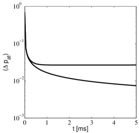
Figure 1: Uncertainty of $p_{\text{at}}$ as function of time. The effective coupling is $\kappa^{2}=1.83\times 10^{6}$ s^-1. The lower curve is without inclusion of atomic decay, and the upper curve includes atomic decay with a rate $\eta=1.7577$ s^-1 and photon absorption with $\epsilon=0.028$. These values correspond for example to a 2 mm² interaction area, $2\times 10^{12}$ atoms, $5\times 10^{14}$ photons s^-1, 10 GHz detuning, and 852 nm light, appropriate for the ¹³³Cs($6S_{1/2}(F=4)-6P_{1/2}(F=5))$ transition with decay rate $3.1\times 10^{7}$ s^-1 and corresponding atomic dipole moment $d=2.61\times 10^{-29}$ Cm. Factors of order unity related to the coupling matrix elements among different states of the actual Zeeman substructure are omitted.

Figure 1 shows the spin squeezing as a function of probing time. When atomic decay is not included, the uncertainty in $p_{\text{at}}$ is a monotonically decreasing function with time. When decays are included, a minimum is reached whereafter the degree of squeezing starts to decrease. On the time scale of the figure, which is chosen to reflect realistic experimental time scales, the increase in $\text{Var}(p_{\text{at}})$ is hardly visible. From Eq. (28), we find that the minimum in the variance occurs at the instant of time

$$t_{\text{min}} = \frac{1}{2\beta\kappa^{2}(1-\epsilon)}$$

$$\times \ln\left(\frac{\text{Var}(p_{\text{at,0}})+\frac{\eta}{2\kappa^{2}(1-\epsilon)}-\frac{\beta}{2}}{\text{Var}(p_{\text{at,0}})+\frac{\eta}{2\kappa^{2}(1-\epsilon)}+\frac{\beta}{2}}\frac{4\beta\kappa^{2}(1-\epsilon)}{\eta}\right).$$

In the typical experimental situation, $\eta/2\kappa^{2}(1-\epsilon)\ll 1$ which means that $\beta\simeq\sqrt{2\eta/(1-\epsilon)}/\kappa$. In this case Eq. (IV) simplifies to

$$t_{\text{min}}=\frac{1}{2\sqrt{2\eta(1-\epsilon)}\kappa}\ln\left(\frac{4\sqrt{2(1-\epsilon)}\kappa}{\sqrt{\eta}}\right).$$ (34)

From Eq. (34), we see that $t_{\text{min}}$ decreases for increasing coupling strength $\kappa$, and for increasing decay rate $\eta$. Interestingly, the instant of time for the minimum in the variance is independent of the initial uncertainty in the atomic variable $p_{\text{at}}$.

We may now go back to Eq. (28) and evaluate the value of the variance at time $t_{\text{min}}$. In the regime considered above, and in the figure, we find

$$\Delta p(t_{\text{min}})=\sqrt{\frac{1}{\kappa}\sqrt{\frac{\eta}{2(1-\epsilon)}}}.$$ (35)

This clearly shows that the higher coupling and the lower decay, the better spin squeezing. It is the term linear in $\eta$ in Eq. (28) that is responsible for the ’saturation effect’ in the variance at early times where the exponential is still close to unity, $e^{\eta t}\simeq 1$.

To specify for a given number of atoms, how many photons we need to obtain optimal spin squeezing in time $t_{\text{min}}$ limited perhaps by other experimental constraints, we express $\eta=\Phi\frac{\sigma}{A}\frac{\Gamma^{2}}{\Delta^{2}}$, $\kappa^{2}=\Phi\frac{\sigma}{A}\frac{\Gamma^{2}}{\Delta^{2}}N_{\text{at}}$, and insert in Eq. (34). The slow logarithmic dependence and factors of order unity can be neglected, and we can introduce $\epsilon$ via the relation $\epsilon=N_{\text{at}}\frac{\sigma}{A}\frac{\Gamma^{2}}{\Delta^{2}}$, and find $\Phi t_{\text{min}}\simeq\frac{1}{\epsilon}\sqrt{\frac{A}{\sigma}N_{\text{at}}}$. If we accept photon absorption at the percent level, we obtain

$$\Phi t_{\text{min}}\gtrsim 100\sqrt{\frac{A}{\sigma}}\sqrt{N_{\text{at}}}.$$ (36)

In our case, we have $A/\sigma\simeq 1.7\times 10^{7}$. A realistic upper limit for $t_{\text{min}}$ is 1 ms, and from Eq. (36) it then follows that the photon flux should fulfill

$$\Phi\gtrsim 10^{8}\sqrt{N_{\text{at}}}\frac{1}{\text{s}}.$$ (37)

V Inhomogeneous light-atom coupling

We now consider two scenarios leading to inhomogeneous light-atom coupling, a case recently discussed theoretically in the literature Kuzmich and Kennedy (2004). First, we shall study the case where the coupling is inhomogeneous as a consequence of a variation in the intensity of the light beam across the sample. Second, we shall consider the case of an optically thick sample where the photon field, and therefore the coupling, changes through the atomic sample due to absorption. Both cases are readily handled within the gaussian approximation.

V.1 Case (a): optically thin sample

We consider the case where the atomic gas is divided into, say $n$, slices each with local light-atom coupling strength $\kappa_{i}$. The $2n+2$ column vector of gaussian variables describing the $2n$ collective canonical position and momentum variables for the atoms, and the 2 collective position and momentum variables for the photon field then reads

$${\bm{y}}=(x_{\text{at},1},p_{\text{at},1},\dots,x_{\text{at},n},p_{\text{at},n},x_{\text{ph}},p_{\text{ph}})^{T}.$$ (38)

The generalization of Eq. (5), to the case with inhomogeneous coupling reads

$$H\tau=\hbar\left(\sum_{i=1}^{n}\kappa_{\tau,i}p_{\text{at},i}\right)p_{\text{ph}},$$ (39)

where the summation index covers the different groups of atoms.

To model the effect of an inhomogeneous coupling of the light to the atomic sample, we consider $n=10$ different values of $\kappa^{2}$ chosen uniformly in the interval $[\kappa_{0}^{2}(1-\delta);\kappa_{0}^{2}(1+\delta)]$ with $\delta=\{0,0.1,0.5\}$. In this way, the effective coupling constant $\sqrt{\sum_{j=1}^{n}\kappa_{j}^{2}}$ remains constant while the variance in the coupling constants increases. The values of the coupling strength could, e.g., differ because of the transverse intensity profile of the laser beam. As a consequence, the values of the atomic decay rate $\eta$ (also proportional to intensity) are different in each slice. The measurement is described by the method in Sec. III, and the propagation is given by a modification of Eq. (21)

$$\mathbf{\gamma}(t+\tau)=\mathbf{L}_{\tau}\mathbf{S}_{\tau}\mathbf{\gamma}_{\tau}\mathbf{S}_{\tau}^{\dagger}\mathbf{L}_{\tau}+\mathbf{M}_{\tau}+\mathbf{N},$$ (40)

where the $(2n+2)\times(2n+2)$ matrix $\mathbf{S}_{\tau}$ is obtained from the time evolution of the system as in Sec. III, and where $\mathbf{L_{\tau}}=\text{diag}(\sqrt{1-\eta_{\tau,1}},\sqrt{1-\eta_{\tau,1}},\dots,\sqrt{1-\eta_{\tau,n}},\sqrt{1-\eta_{\tau,n}},\sqrt{1-\epsilon},\sqrt{1-\epsilon})$, $\mathbf{M}_{\tau}=\hbar\times\text{diag}(\frac{N_{\text{at},1}\eta_{1}}{\langle J_{x,1}\rangle},\frac{N_{\text{at},1}\eta_{1}}{\langle J_{x,1}\rangle},\dots,\frac{N_{\text{at},n}\eta_{n}}{\langle J_{x,n}\rangle},\frac{N_{\text{at},n},\eta_{n}}{\langle J_{x,n}\rangle},0,0)$, and $\mathbf{N}=\text{diag}(0,0,\dots,0,0,\epsilon,\epsilon)$. For convenience, we assume that the number of atoms $N_{at,i}$ subject to a given coupling strength $\kappa_{i}$ is simply $N_{\text{at}}/n$.

The atomic covariance matrix now has dimension $(2n\times 2n)$, and it contains the variances of the atomic observables in each slice and the correlations between them. Collective observables are described by linear combinations of the $(x_{at,i},p_{at,i})$ and their variances can be obtained explicitly.

From the Hamiltonian (39), it is clear, that the probe field couples to the asymmetric collective variable $\sum_{i=1}^{n}\kappa_{\tau,i}p_{\text{at},i}$. The corresponding asymmetric collective harmonic oscillator variables involved in the spin squeezing are, accordingly

$$(X_{\text{eff}},P_{\text{eff}})=\left(\frac{\sum_{i=1}^{n}\kappa_{i}x_{\text{at},i}}{\sqrt{\sum_{i=1}^{n}\kappa_{i}^{2}}},\frac{\sum_{i=1}^{n}\kappa_{i}p_{\text{at},i}}{\sqrt{\sum_{i=1}^{n}\kappa_{i}^{2}}}\right),$$ (41)

The symmetric collective variables that are usually considered (see, e.g., the discussion in Ref. Kuzmich and Kennedy (2004) and references therein), are, on the other hand, given by

$$(X,P)=\left(\frac{1}{\sqrt{n}}\sum_{i=1}^{n}x_{\text{at},i},\frac{1}{\sqrt{n}}\sum_{i=1}^{n}p_{\text{at},i}\right),$$ (42)

and it is interesting to see how these two sets of variables are connected. A straightforward calculation shows that we may express the latter variables as

$$(X,P)=a(X_{\text{eff}},P_{\text{eff}})+b(X_{\bot},P_{\bot}),$$ (43)

where $(X_{\bot},P_{\bot})$ are canonical variables which commute with ($X_{\text{eff}},P_{\text{eff}}$) and with the interaction Hamiltonian of Eq. (33), and where the coefficients are given by

$$a=\frac{\sum_{j=1}^{n}\kappa_{j}/\sqrt{n}}{\sqrt{\sum_{j=1}^{n}\kappa_{j}^{2}}},$$ (44)

and

$$b(X_{\bot},P_{\bot})=\frac{1}{\sqrt{n}}\sum_{i=1}^{n}\left(1-\frac{\kappa_{i}\sum_{j=1}^{n}\kappa_{j}}{\sum_{j=1}^{n}\kappa_{j}^{2}}\right)(x_{\text{at},i},p_{\text{at},i}).$$ (45)

From Eq. (43), it follows that the variances of $X$ and $P$ may be expressed as

$$\text{Var}(X)=a^{2}\text{Var}(X_{\text{eff}})+(1-a^{2})/2,$$ (46)

and

$$\text{Var}(P)=a^{2}\text{Var}(P_{\text{eff}})+(1-a^{2})/2,$$ (47)

where we have used that $1=a^{2}+b^{2}$ and that the components $(X_{\bot},P_{\bot})$ are unaffected by measurements, so $\text{Var}(X_{\bot})=\text{Var}(P_{\bot})=1/2$ for all times (if atomic decay is not taken into account).

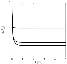
Figure 2: Uncertainty of the maximally squeezed component of the atomic gas ($P_{\text{at}}$) as function of time. The higher-lying curves show the uncertainty in the symmetric collective parameter (Eq. (42)) for $n=10$ uniformly distributed values of $\kappa^{2}$ in $[0.9\kappa_{0}^{2};1.1\kappa_{0}^{2}]$ (middle) and $[0.5\kappa_{0}^{2};1.5\kappa_{0}^{2}]$ (upper) . The central effective coupling is $\kappa_{0}^{2}=1.83\times 10^{6}$ s^-1, and all other parameters are as in Fig. 1. The lower curve is the smallest eigenvalue of the covariance matrix, which is the same for the two ranges of $\kappa^{2}$ to the precision visible in the figure.

In Fig. 2, the lowest curve shows the smallest eigenvalue of the covariance matrix as a function of time. The associated eigenvector represents a combination of the canonical variables for the different slices, which is maximally squeezed. For the present values of the noise parameters ($\eta$ and $\epsilon$), we have an overlap very close to unity between the eigenvector of this curve and the effective asymmetric collective variable $P_{\text{eff}}$ of Eq. (41). This means that this component is indeed the one that is maximally squeezed. The analytical result for the squeezing of this component is obtained from (32) with $\kappa\rightarrow\sqrt{\sum_{j=1}^{n}\kappa_{j}^{2}}$. For the values for atomic decay and photon absorption considered in the figure, also the formula (47) reproduces the fully numerical calculations for the symmetric collective coordinate $P$ of Eq. (42).

V.2 Case (b): optically thick gas

We now turn to the situation where the sample is optically thick. The probability $\epsilon$ for absorption of photons through the gas is then larger than, say, a few percent. This means that the condition $\epsilon\ll 1$ which was assumed in the derivation of the effective light-atom coupling of Eq. (5) is no longer fulfilled. By slicing the gas into pieces labeled by $i=1,2,\dots,n$, within each of which the constraint on atomic decay and photon absorption $\eta_{i},\epsilon_{i}\ll 1$ is fulfilled, we may, however, still locally for a fixed slice $i$ use the effective Hamiltonian and address the problem in the gaussian approximation. The vector of variables describing the system is then of the same form as in Eq. (38), and the Hamiltonian is given by Eq. (39). The considerable absorption of photons from a beam segment on its way through the atomic gas, means that the update formula for the covariance matrix needs to be iterated according to the different local noise and coupling strengths. Accordingly, as each beam segment passes through the atomic gas for $i=1$ to $n$, we go through the following update formulae for the covariance matrix (21):

$$\bm{\gamma}_{i} = \mathbf{L}_{\tau,i}\mathbf{S}_{\tau,i}\bm{\gamma}_{i-1}\mathbf{S}^{T}_{\tau,i}\mathbf{L}_{\tau,i}$$

$$+ \frac{\hbar N_{\text{at},i}}{\langle J_{x,i}(t)\rangle}\mathbf{M}_{\tau,i}+\frac{\hbar N_{\text{ph},i}}{2\langle S_{x,i}(t)\rangle}\mathbf{N}_{i}$$

where the transformation matrix $\mathbf{S}_{\tau,i}$ is given by a matrix with off-diagonal elements $\kappa_{\tau,i}$ at entrances $((2i-1),(2n+2))$ and $((2n+1),2i))$. For example, $\mathbf{S}_{\tau,2}$ for the case of only two slices ($n=2$) is given by

$$\mathbf{S}_{\tau,2}=\left(\begin{array}[]{cccccc}1&0&0&0&0&0\\ 0&1&0&0&0&0\\ 0&0&1&0&0&\kappa_{\tau,2}\\ 0&0&0&1&0&0\\ 0&0&0&\kappa_{\tau,2}&1&0\\ 0&0&0&0&0&1\\ \end{array}\right).$$ (55)

The constraints on decay and absorption must be fulfilled $\eta_{\tau,i},\epsilon_{i}\ll 1$ and $\mathbf{L}_{\tau,i}=\text{diag}(1,\dots,\sqrt{1-\eta_{\tau,i}},\sqrt{1-\eta_{\tau,i}},1,\dots,\sqrt{1-\epsilon_{i}},\sqrt{1-\epsilon_{i}})$, $\mathbf{M}_{\tau,i}=\text{diag}(0,\dots,0,\eta_{\tau,i},\eta_{\tau,i},0,\dots,0))$., and $\mathbf{N}_{i}=\text{diag}(0,\dots,0,\epsilon_{i},\epsilon_{i})$. The full covariance matrix is updated every time the pulse segment passes a new slice. When the pulse segment has finally left the gas, it is being measured, and $\bm{\gamma}_{n}$ is modified ($\bm{\gamma}_{n}\rightarrow\bm{\gamma}_{n}^{\prime})$ according to Eqs. (18) and (19) of Sec. III, with the $2n\times 2n$ submatrix $\mathbf{A_{\gamma}}$ the covariance matrix for the variables $\bm{y}_{1}=(x_{\text{at},1},p_{\text{at},1},\dots,x_{\text{at},n},p_{\text{at},n})^{T}$, $\mathbf{B_{\gamma}}$ the $2\times 2$ covariance matrix for $\bm{y}_{2}=(x_{\text{ph}},p_{\text{ph}})^{T}$ and $\mathbf{C_{\gamma}}$ the $2n\times 2$ correlation matrix for $\bm{y}_{1}$ and $\bm{y}_{2}^{T}$. When we set $\bm{\gamma}_{0}(t+\tau)=\bm{\gamma}_{n}^{\prime}(t)$, we use Eq. (V.2) with $i=1$ to $n$ to describe the interaction with the next beam segment. In reality, the light segment corresponding to any practical duration $\tau$ will be much longer than the entire atomic sample, and the interaction with one group of atoms has not finished before the interaction with the subsequent group starts. It is not difficult to see, however, that if the atomic dynamics is entirely due to the interaction with the optical field, there is no difference between the achievements of the real system and those where we imagine the atomic slices separated by free space separation distances larger than $c\tau$, described precisely by the above formulation. In Eq. (V.2),

For convenience, we give the time and space (slice) dependence of the parameters in Eqs. (V.2) and (55) explicitly. The change in the classical Stokes vector through the different slices due to photon absorption is given by

$$\langle S_{x,i}\rangle=\langle S_{x,i=0}\rangle\exp(-\sum_{i^{\prime}=1}^{i}\epsilon_{i^{\prime}}),$$ (56)

where the absorption probability in slice $i$ is $\epsilon_{i}$, and hence the total photon absorption probability in the gas is $(1-\exp(-\sum_{i=1}^{n}\epsilon_{i}))$. The change in $\langle J_{x,i}\rangle$ due to atomic decay is given by

$$\langle J_{x,i}(t)\rangle=\langle J_{x,i}(0)\rangle\exp(-\eta_{i}t).$$ (57)

The atomic decay rate $\eta_{i}$ is a decreasing function of the slice-number since fewer and fewer photons are available to excite the atoms

$$\eta_{i}=\eta_{0}\exp(-\sum_{i^{\prime}=1}^{i}\epsilon_{i^{\prime}}),$$ (58)

and finally, the light-atom coupling constant $\kappa$ will depend on both time and space

$$\kappa^{2}(t,i)=\kappa_{0}^{2}\exp(-\sum_{i^{\prime}=1}^{i}\epsilon_{i^{\prime}})\exp(-\eta_{i}t),$$ (59)

where $\kappa_{0}^{2}$ is given as in Eq. (29) and every slice contains $N_{\text{at},i}=N_{\text{at}}$ atoms. From the above relations and the initial conditions $\langle S_{x,i}\rangle=\hbar N_{\text{ph},i}/2$ and $\langle J_{x,i}\rangle=\hbar N_{\text{at},i}/2$ it follows that the pre-factors on the noise terms in Eq. (V.2) are given by

$$\frac{\hbar N_{\text{at},i}}{\langle J_{x,i}\rangle}=\frac{2}{e^{-\eta_{i}t}},$$ (60)

and

$$\frac{\hbar N_{\text{ph},i}}{2\langle S_{x,i}\rangle}=\frac{1}{e^{-\sum_{i^{\prime}=1}^{i}\epsilon_{i^{\prime}}}}.$$ (61)

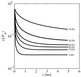
Figure 3: Uncertainty of the maximally squeezed component of the gas ($P_{\text{at}}$) as function of probing time for varying degrees of photon absorption. The percentage of photons absorbed is indicated at the solid curves. The gas is decomposed in $n$ slices each absorbing $\epsilon_{i}=0.028$ of the light intensity. From the lower to the upper curve the number of such slices attains the values $n=1,4,8,13,25$, and 50. Other physical parameters are as specified in Fig. 1.

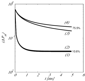
Figure 4: As Fig. 3 but only for $n=4$ and $n=50$. Curves (1) and (3) represent the maximally squeezed component of the gas. Curves (2) and (4) display the uncertainty in the inhomogeneous collective variable $P_{\text{eff}}$ of Eq. (41) as a function of time.

We have modeled the effect of photon-absorption induced inhomogeneous light-atom coupling using the parameters detailed in the caption of Fig. 3. The photon absorption is varied by varying the detuning, and the light-atom coupling strength $\kappa^{2}$ and the atomic decay probability $\eta$ are kept constant at the values used in Figs. 1 and 2 by adjusting the photon flux inversely proportional to changes in the detuning squared. Figure 3 shows the uncertainty of the maximally squeezed component of the sample as determined by the smallest eigenvalue of the covariance matrix. We see as expected that the degree of squeezing decreases with increasing photon absorption probability.

In Fig. 4, we compare for two representative cases from Fig. 3, the uncertainty of the maximally squeezed component of the gas with the uncertainty of the collective inhomogeneous variable $P_{\text{eff}}$ of Eq. (41). The variance of the latter variable can be calculated straightforwardly from our knowledge of the time-dependent light-atom coupling constants $\kappa_{i}$ and the full covariance matrix: $\text{Var}(P_{\text{eff}})=\left(\sum_{i,j}\kappa_{i}(t)\kappa_{j}(t)(\langle p_{i}p_{j}\rangle-\langle p_{i}\rangle\langle p_{j}\rangle)\right)\big{/}\sum_{k}\kappa_{i}(t)^{2}$. We see that for low and moderate photon absorption, the result for the effective asymmetric variable of Eq. (41) is close to the fully numerical result. Only for high photon absorption the effects of noise and differences in coupling strength lead to a significant deviation from the numerical result.

VI Probing the degree of squeezing

So far, we have not discussed to which extent the maximally squeezed component of the atomic sample will be useful and, e.g., set the limit for the precision obtained in a measurement of an interesting physical quantity. To investigate this point, we follow the work in Ref. Kuzmich and Kennedy (2004), and consider a situation where (i) the sample is spin squeezed for a time periode $t_{1}$ (ii) the spin squeezing is stopped, and the sample is subject to a spin rotation, and (iii) the system is probed, and the rotation angle is determined.

VI.1 Noiseless case: Analytical results

We start by an analysis of the simple case corresponding to a single atomic sample and a single probe field in the noise-less limit. From Sec. III, we have at time $t_{1}$

$$\text{Var}(p_{\text{at}}(t_{1}))=\frac{1}{2\kappa^{2}t_{1}+2},$$ (62)

where we have used that the atoms are initially in a coherent state with variance $1/2$. Since $\text{Var}(x_{\text{at}})\text{Var}(p_{\text{at}})=1/4$ in this noiseless case, we also have

$$\text{Var}(x_{\text{at}}(t_{1}))=\kappa^{2}t_{1}/2+1/2.$$ (63)

After the time $t_{1}$, the light-atom coupling is turned off, and the system is subject to a rotation around the $y$ axis, described by the interaction $HT=-\theta J_{y}$, where $\theta=\omega T$ is the small angle of rotation resulting from the action of the constant rotation frequency $\omega$ in time $T$, and where $J_{y}$ is the $y$ component of the collective spin operator. Making the translation to the effective dimensionless position operator as in Eq. (4) leads to the Hamiltonian

$$HT=-\hbar\theta\alpha x_{\text{at}},$$ (64)

where $\alpha=\sqrt{\langle J_{x}\rangle/\hbar}=\sqrt{\frac{N_{\text{at}}}{2}}$. To obtain an estimate for the unknown classical variable $\theta$, we follow the ideas introduced in Ref. Mølmer and Madsen (2004), and treat the rotation variable $\theta$ as a quantum variable within our gaussian description. The total system is then described by two atomic variables and one rotation variable $\bm{y}=(\theta,x_{at},p_{at})^{T}$. The corresponding transformation matrix follows from Heisenbergs equations of motion with the Hamiltonian in Eq. (64) and in the basis ($\theta,x_{\text{at}},p_{\text{at}}$) we obtain

$$\mathbf{S}=\left(\begin{array}[]{ccc}1&0&0\\ 0&1&0\\ \alpha&0&1\\ \end{array}\right).$$ (68)

from which we verify that, e.g, $p_{\text{at}}\rightarrow p_{\text{at}}+\alpha\theta$. Equation (13) now determines the time-evolution of the system, and we find the following covariance matrix at time $t_{2}$ after the rotation:

$$\mathbf{\gamma}(t_{2})=\left(\begin{array}[]{ccc}2\text{Var}(\theta_{0})&0&\alpha 2\text{Var}(\theta_{0})\\ 0&2\text{Var}(x_{\text{at}}(t_{1}))&0\\ \alpha 2\text{Var}(\theta_{0})&0&2\text{Var}(p_{\text{at}}(t_{1}))+\alpha^{2}2\text{Var}(\theta_{0})\\ \end{array}\right),$$ (72)

where $\text{Var}(p_{\text{at}}(t_{1}))$ and $\text{Var}(x_{\text{at}}(t_{1}))$ are given by Eqs. (62) and (63), respectively.

Finally, at times $t\geq t_{2}$, the rotation is turned off, and the sample is probed by the light beam as in the time interval $[0;t_{1}]$. The transformation matrix is determined by Heisenberg’s equations of motion for the variables $\bm{y}=(\theta,x_{\text{at}},p_{\text{at}},x_{\text{ph}},p_{\text{ph}})^{T}$ with the Hamiltonian (5) and is given by

$$\mathbf{S}=\left(\begin{array}[]{ccccc}1&0&0&0&0\\ 0&1&0&0&\kappa\\ 0&0&1&0&0\\ 0&0&\kappa&1&0\\ 0&0&0&0&0\\ \end{array}\right).$$ (78)

The covariance matrix of the system is propagated according to Eq. (13). The measurements on the photon field are described as in Eqs. (24) and (25) (see also Ref. Mølmer and Madsen (2004)). The submatrix $\mathbf{A}_{\gamma}$ is now the $3\times 3$ matrix pertaining to the variables ($\theta,x_{\text{at}},p_{\text{at}}$), and $\mathbf{C}_{\gamma}$ is the $3\times 2$ covariance submatrix describing the coherences and correlations between these three variables and the photon field. We are interested in the uncertainty on the value of $\theta$, i.e., the (1,1) entrance in the covariance matrix. To find this as a function of time, we follow the procedure in Sec. III and calculate the difference between $\mathbf{A}_{\gamma}$ after $n$ and $n+1$ iterations, and consider the limit of infinitesimal time steps. In general, the differential equations obtained in this way are matrix Ricatti equations and may be solved in standard ways Stockton et al. (2004). In the present case, the solution reads for probing times $t\geq t_{2}$:

$$\text{Var}(\theta(t))=\text{Var}(\theta_{0})-\frac{\text{Re}(\langle(\theta-\langle\theta\rangle)(p_{at}-\langle p_{at}\rangle)\rangle_{t_{2}})}{\text{Var}(p(t_{2}))}\left(1-\frac{1}{\left(1+2\text{Var}(p(t_{2}))\kappa^{2}(t-t_{2})\right)}\right),$$ (79)

where the covariances at time $t_{2}$ are given in Eq. (72). We see from Eq. (79) that the variance of the variable $\theta$ does not decrease forever. In the long time limit, we find

$$\text{Var}(\theta(t\rightarrow\infty))=\text{Var}(\theta_{0})\left(\frac{\text{Var}(p_{\text{at}}(t_{1}))}{\text{Var}(p_{\text{at}}(t_{1}))+\alpha^{2}\text{Var}(\theta_{0})}\right).$$ (80)

This shows, as expected, that the limiting value only depends on the squeezing and the rotation until time $t_{2}$. For large $\alpha$ parameter (many atoms) and for a sufficiently large initial variance of $\theta$, the result in Eq. (80) reduces to

$$\text{Var}(\theta)\simeq\frac{\text{Var}(p_{\text{at}}(t_{1}))}{\alpha^{2}}.$$ (81)

The ratio of the variances of $\theta$ in a measurement with (S) and without (NS) spin squeezing is given by

$$\frac{\text{Var}(\theta^{\text{S}})}{\text{Var}(\theta^{\text{NS}})}=2\text{Var}(p^{\text{S}}_{\text{at}}(t_{1}))$$ (82)

Since $\text{Var}(p_{\text{at}}(t_{1}))\in]0;1/2]$ this shows that one may gain a significant factor in precision on the variable $\theta$ by pre-squeezing the sample.

Finally, we note that the result of Eq. (80) may be obtained directly by considering the corresponding classical gaussian probability distribution $P(p_{\text{at}},\theta)\propto\exp\left(-p_{\text{at}}^{2}/(2\text{Var}(p_{\text{at}}))-\theta^{2}/(2\text{Var}(\theta))\right)$. As a consequence of the rotation, $p_{\text{at}}$ transforms according to $p_{\text{at}}\rightarrow p_{\text{at}}+\alpha\theta$, and therefore the probability distribution after rotation reads $P(p_{\text{at}},\theta)\propto\exp\left(-(p_{\text{at}}-\alpha\theta)^{2}/(2\text{Var}(p_{\text{at}}))-\theta^{2}/(2\text{Var}(\theta))\right)$. A measurement of the variable $p_{\text{at}}$ leads to a distribution in $\theta$ only, from which the variance of $\theta$ is read off with the result given in Eq. (80).

VI.2 Noise included: Numerical results

Whereas in Sec. VI.1 it is clear that it is the collective variable $p_{\text{at}}$ that is squeezed, in the case of an atomic ensemble with an inhomogeneous light-atom coupling we only know from the analysis of Secs. V.1 and V.2 that there exists a component that is squeezed, and that this component for moderate noise is very accurately approximated by the asymmetric collective variable $P_{\text{eff}}$ of Eq. (41). The question we address now is whether it is the variance of this component that will show up in a measurement of a classical parameter, such as the rotation parameter $\theta$.

The formalism necessary for handling this problem was developed in Secs. III and V.2. In short, for $n$ slices of gas each fulfilling $\epsilon_{i},\eta_{i}\ll 1$, ($i=1,\dots,n$) we first propagate and perform measurements on the system of $2n$ collective atomic position and momentum variables and 2 collective photon position and momentum variables. At time $t_{1}$, the light field is turned off, and the atomic sample is for $t\in[t_{1};t_{2}]$ subject to a rotation around the $y$ axis described by the effective Hamiltonian

$$H\tau=-\hbar\theta\sum_{i}^{n}\alpha_{i}x_{\text{at},i},$$ (83)

with $\theta=\omega T$ as in Sec. VI.1 and with coupling constants $\alpha_{i}$ determined by a generalization of the result in Eq. (64)

$$\alpha_{i}=\sqrt{\frac{\langle J_{x,i}\rangle}{\hbar}}=\sqrt{\frac{N_{\text{at},i}}{2}e^{-\eta_{i}t_{1}}}.$$ (84)

Spontaneous emission of photons is neglected in our approach, so the $\alpha_{i}$’s are fixed by their values at the instant of time $t_{1}$ when the photon field is switched off, and the possibility for stimulated atomic decay disappears. The transformation matrix $\mathbf{S}$ corresponding to the Hamiltonian in Eq. (83) is readily found from Heisenberg’s equations of motion for the variables ($\theta,x_{\text{at},1},p_{\text{at},1},\dots,x_{\text{at},n},p_{\text{at},n}$). Its diagonal entries are unity, the $i=1,\dots,n$ $(\theta,p_{\text{at},i})$ entries are assigned the values $\alpha_{i}$, and the rest are zero; a natural generalization of Eq. (68). The propagation in time of the covariance matrix is then determined by Eq. (13). At time $t_{2}$ the rotation is stopped, and for times $t>t_{2}$, the atom-light Hamiltonian is turned on again. First the initial covariance matrix for $\theta$, atomic slices and the photon field ($\theta,x_{\text{at},1},p_{\text{at},1},\dots,x_{\text{at},n},p_{\text{at},n},x_{\text{ph}},p_{\text{ph}}$) is set up. This involves the covariance from the previous part supplemented by the position and momentum variables of the photon field. The dynamics of this enlarged covariance matrix is described by suitable modified versions of Eqs. (17) and (19) of Sec. III.

propagation with this enlarged covariance matrix is performed by the standard equation of Sec. III properly adjusting the transformation matrix and the matrices associated with noise.

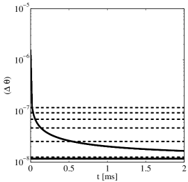
Figure 5: Uncertainty of the parameter $\theta$ as a function of time and for different variances of the coupling strength as specified in the text. The gas is sliced in $n=10$ pieces. The number of atoms and photons are as in the preceding figures. The value of $\alpha_{i}$ is 0.2236. The dashed curves show the limiting uncertainty in the $\theta$ parameter as estimated from Eq. (88) for the standard collective variable $P$ of Eq. (42) with the smallest variance in the coupling strength for the lowest dashed curve and the highest variance for the upper dashed curve. The constant horizontal solid line gives the limiting value of Eq. (64), as obtained by the maximally squeezed component $P_{\text{eff}}$ of Eq. (41), and it is independent of the variance of the coupling strength. The decreasing full curve is a collection of indistinguishable curves showing the numerical results for all the different variances of the coupling strength (see text).

We aim to extract from our numerical study that the variable of relevance in the probing of the rotation angle is the maximally squeezed component, i.e., at moderate noise levels it is essentially the optimally squeezed asymmetric $P_{\text{eff}}$ variable of Eq. (41) and not the symmetric collective variable $P$ of Eq. (42). From Heisenberg’s equation of motion it follows that $P_{\text{eff}}$ and $P$ transform according to

$$P_{\text{eff}}\rightarrow P_{\text{eff}}+\left(\frac{\sum_{j=1}^{n}\kappa_{j}\alpha_{j}}{\sqrt{\sum_{j=1}^{n}\kappa_{j}^{2}}}\right)\theta,$$ (85)

and

$$P\rightarrow P+\left(\frac{\sum_{j=1}^{n}\alpha_{j}}{\sqrt{n}}\right)\theta.$$ (86)

A generalization of the result in Eq. (81) then yields the following expressions for the variance of $\theta$ in the long time limit

$$\text{Var}(\theta)=\frac{\text{Var}(P_{\text{eff}})}{\left(\frac{\sum_{j=1}^{n}\kappa_{j}\alpha_{j}}{\sqrt{\sum_{j=1}^{n}\kappa_{j}^{2}}}\right)^{2}},$$ (87)

and

$$\text{Var}(\theta^{\prime})=\frac{\text{Var}(P)}{\left(\frac{\sum_{j=1}^{n}\alpha_{j}}{\sqrt{n}}\right)^{2}},$$ (88)

where $\text{Var}(P)$ is given by Eq. (47).

Figure 5 shows results for inhomogeneous coupling modeled by choosing $n=10$ different values of $\kappa^{2}$ uniformly over the interval $[(1-\delta)\kappa_{0}^{2}/n;(1+\delta)\kappa_{0}^{2}/n]$ with $\delta\in\{0,0.02,0.1,0.2,0.3,0.4,0.5\}$. As in Sec. V, the effective coupling strength is fixed by $\kappa_{0}$. In the figure, the solid lines are independent of fluctuations in the coupling strength. The lowest solid line shows the asymptotic uncertainty of $\theta$ as obtained by Eq. (87). The decreasing solid curve is the numerical result, converging towards this value. It represents a collection of indistinguishable curves showing the numerical results for all the different variances of the coupling strength. We observe that the decreasing solid curves show a better estimation of the rotation angle $\theta$ than the prediction by the symmetric collective variable shown by the dashed curves in the figure. The fact that the decreasing full curves converge to the value determined by the maximally squeezed component signifies that this indeed sets the limit for the precision of the measurement.

VII Conclusions

In this work we have given a comprehensive account of the theory of probing and measurements in the gaussian state approximation. We have followed the ideas of Refs. Mølmer and Madsen (2004); Hammerer et al. (2003), and we have provided a complete analysis of the method and its strengths by analyzing in detail the problem of spin squeezing.

The gaussian approximation for the collective quantum parameters including possibly an external classical parameter allows us to include the measurement process directly, and to obtain analytical results in the noise-less case and in the limit of low noise. Also the theory is readily generalized to handle situations which have resisted a satisfactory treatment with other theoretical methods. For example, the case of an optically thick gas with corresponding inhomogeneous light-atom coupling can be treated and even understood analytically to a large extent.

We have shown that in the present case of squeezing of the spin of an atomic ensemble by using a continuous wave coherent light beam, it is indeed the maximally squeezed component of the atomic gas that determines the precision with which one can estimate the value of an external perturbation.

At present, we seek to address a series of other problems in continuous variable quantum physics including generation and detection of finite band-width squeezed light and estimation of time-varying external perturbations.

References

- Geremia et al. (2003) J. M. Geremia, J. K. Stockton, A. C. Doherty, and H. Mabuchi, Phys. Rev. Lett. 91, 250801 (2003).
- Mølmer and Madsen (2004) K. Mølmer and L. B. Madsen, quant-ph/0402158 (2004).
- Duan et al. (2000) L. M. Duan, J. I. Cirac, P. Zoller, and E. S. Polzik, Phys. Rev. Lett. 85, 5643 (2000).
- Julsgaard et al. (2001) B. Julsgaard, A. Kozhekin, and E. S. Polzik, Nature 413, 400 (2001).
- Kuzmich et al. (1998) A. Kuzmich, N. P. Bigelow, and L. Mandel, Europhys. Lett. 42, 481 (1998).
- Takahasi et al. (1999) Y. Takahasi, K. Honda, N. Tanaka, K. Toyoda, K. Ishikawa, and T. Yabuzaki, Phys. Rev. A 60, 4974 (1999).
- Kuzmich et al. (1999) A. Kuzmich, L. Mandel, J. Janis, Y. E. Young, R. Ejnisman, and N. P. Bigelow, Phys. Rev. A 60, 2346 (1999).
- Bouchoule and Mølmer (2002) I. Bouchoule and K. Mølmer, Phys. Rev. A 66, 043811 (2002).
- Muller et al. (2004) J. H. Muller, P. Petrov, D. Oblak, C. L. G. Alzar, S. R. de Echaniz, and E. S. Polzik, quant-ph/0403138 (2004).
- Thomsen et al. (2002) L. K. Thomsen, S. Mancini, and H. M. Wiseman, J. Phys. B: At. Mol. Opt. Phys. 35, 4937 (2002).
- Kuzmich and Kennedy (2004) A. Kuzmich and T. A. B. Kennedy, Phys. Rev. Lett. 92, 030407 (2004).
- Geremia et al. (2004) J. M. Geremia, J. K. Stockton, and H. Mabuchi, Science 304, 270 (2004).
- Kraus et al. (2003) B. Kraus, K. Hammerer, G. Giedke, and J. I. Cirac, Phys. Rev. A 67, 042314 (2003).
- Hammerer et al. (2003) K. Hammerer, K. Mølmer, E. S. Polzik, and J. I. Cirac, quant-ph/0312156 (2003).
- Giedke and Cirac (2002) G. Giedke and J. I. Cirac, Phys. Rev. A 66, 032316 (2002).
- Fiurášek (2002) J. Fiurášek, Phys. Rev. Lett. 89, 137904 (2002).
- Eisert and Plenio (2003) J. Eisert and M. B. Plenio, International Journal of Quantum Information, Vol. 1, No. 4 (2003) 479,quant-ph/0312071 (2003).
- Sherson and Mølmer (2004) J. Sherson and K. Mølmer, in preparation (2004).
- Maybeck (1979) P. S. Maybeck, Stochastic Models, Estimation and Control. Volume 1 (Academic Press: New York, 1979).
- Stockton et al. (2004) J. K. Stockton, J. M. Geremia, A. C. Doherty, and H. Mabuchi, Phys. Rev. A 69, 032109 (2004).