Quantum computation with cold bosonic atoms in an optical lattice

Abstract

Quantum computing, adiabatic, cold atoms, optical lattice. We analyse an implementation of a quantum computer using bosonic atoms in an optical lattice. We show that, even though the number of atoms per site and the tunneling rate between neighbouring sites is unknown, one may perform a universal set of gates by means of adiabatic passage.

1 Introduction

Some tasks in Quantum Information require the implementation of quantum gates with a very high fidelity (A. M. Steane 2002; E. Knill 1998; D. Aharonov 1999). This implies that all parameters describing the physical system on which the computer is implemented have to be controlled with a very high precision, something which it is very hard to achieve in practice.

For example one can imagine an implementation in which qubits are stored in atoms and are manipulated using Raman transitions. It may happen that the relative phase of the lasers driving a Raman transition can be controlled very precisely, whereas the corresponding Rabi frequency $\Omega$ has a larger uncertainty $\Delta\Omega$. If we denote by $T$ the time required to execute a local gate (of the order of $\Omega^{-1}$), then a high gate fidelity requires $T\Delta\Omega\ll 1$ (equivalently, $\Delta\Omega/\Omega\ll 1$), which may very hard to achieve, at least to reach the above mentioned threshold.

In this paper we analyse an implementation of quantum computing using atoms confined in optical lattices. These systems have interesting features for quantum computing. Namely, a large number of atoms can be trapped in the lattice at a very low temperature, which provides a large number of qubits. Also, neutral atoms interact weakly with the environment, which leads to a relatively slow decoherence. However, the same setups pose also important experimental challenges, such as being able to load the lattice with one atom per site or being able to measure the interaction and tunneling constants of these systems with high accuracy. These obstacles, together with the uncertainties in the atom-laser interaction, must be overcome to implement current proposals for quantum computing with neutral atoms (D. Jaksch 1999; R. Ionicioiu 2002).

In this paper we analyse a way that solves the above mentioned problems and show how to achieve a very high gate fidelity even when most of the parameters describing the atomic ensemble (number of atoms per lattice site, tunneling rate, Rabi frequencies, etc) cannot be adjusted to precise values, and even have uncertainties of the order of the parameters themselves.

Our method combines the technique of adiabatic passage with ideas of quantum control theory. The use of adiabatic passage to implement quantum gates is not a new idea, and indeed several methods based on Berry phases have been proposed recently (P. Zanardi 1999; J. Pachos 2000; J. A. Jones 1999; G. Falci 2000; L.-M. Duan 2001). Furthermore, adiabatic passage techniques have been suggested as a way of implementing a universal set of holonomies (L.-M. Duan 2001), i.e. quantum gates which are carried out by varying certain parameters and whose outcome only depends on geometrical properties of the paths in parameter space (P. Zanardi 1999; J. Pachos 2000). However, all these proposals are based on the existence of holonomies in the system, which in turn implies a huge degeneracy in the system. This will not be the case in our scheme.

The outline of the paper is as follows. In §2 we introduce the requirements for quantum computing and show which tools are available in current experiments with cold atoms in optical lattices. We will demonstrate that, due to imperfections in the loading of the lattice, the Hamiltonian of the system is not known with enough accuracy to perform quantum computing in a ‘traditional’ way. In §3 we develop a technique to circumvent our ignorance about the Hamiltonian. Performing adiabatic passage with the different parameters of our problem, we show how to produce a universal set of gates (Hadamard, phase, and CNOT). In §4 we quantify the errors of our proposal, studying the influence of the speed of the adiabatic process, and of other imperfections. In §5 we summarize our results and offer some conclusions.

2 Cold bosonic atoms in optical lattices

We will consider a set of bosonic atoms confined in a periodic optical lattice at sufficiently low temperature such that only the first Bloch band is occupied. The atoms have two relevant internal (ground) levels, $|{a}\rangle$ and $|{b}\rangle$, and we wish to use this degree of freedom to store the qubit. This set-up has been studied in D. Jaksch (1999) where it has been shown how single quantum gates can be realized using lasers and two–qubit gates by displacing the atoms that are in a particular internal state to the next neighbour location. The basic ingredients of such a proposal have been recently realized experimentally (I. Bloch 2002, personal communication). However, in this and all other schemes so far (E. Charron 2002; K. Eckert 2002) it is assumed that there is a single atom per lattice site since otherwise even the concept of qubit is no longer valid. In present experiments, in which the optical lattice is loaded with a Bose-Einstein condensate (D. Jaksch 1998; M. Greiner 2002), this only approximately true, since zero temperature is required and the number of atoms must be identical to the number of lattice sites.

2.1 Requirements for computation

The uncertainty of the number of atoms per lattice site poses severe problems. Having $n_{i}$ atoms on the $i$-th cell, the configuration of this lattice size will be given by a combination of $n_{i}+1$ possible states

$${\cal H}_{i}=\mathrm{lin}\left\{\frac{1}{\sqrt{n_{i}!(n_{i}-k)!}}{b^{\dagger}_{i}}^{k}{a^{\dagger}_{i}}^{n_{i}-k}|{vac}\rangle_{i},\quad k=0\ldots n_{i}\right\}.$$ (1)

To do quantum computing with $m$ qubits, we must find a $2^{m}$-dimensional subspace ${\cal H}_{c}\subset{\cal H}_{1}\otimes\cdots\otimes{\cal H}_{m}$, which is energetically separated from the rest, so that once we set our computer in a superposition of qubits $|{0}\rangle$ and $|{1}\rangle$, it does not leave this subspace. A second, and stronger requirement is that our computation space must be an eigenspace of our Hamiltonian, with the same eigenvalue

$$H(|{z_{1}}\rangle\otimes\cdots\otimes|{z_{n}}\rangle)=0,\quad\forall z_{i}\in\mathbb{Z}_{2},$$ (2)

which we assume 0. Otherwise the trivial evolution of our system would spoil the quantum computation by introducing uncontrollable, unknown phases.

Right from the beginning we forsee several difficulties. First, for arbitrary interactions, the states with different occupation numbers (1) will be regularly spaced and we will not be able to select our qubits. Furthermore, even if we customize the interactions between bosons, given that we basically ignore the number of atoms per site, $n_{i}$, a basic requisite of our scheme will be to show that our procedure works independently of the occupation numbers. Both problems cannot be solved in general. We will rather have to impose some restrictions on our physical system, and this is the purpose of the following subsections.

2.2 Definition of qubit

A crucial assumption which is suggested by the requirement (2), is to impose that the atoms in internal state $|{a}\rangle$ do not interact and do not hop to neighbouring sites. In the absence of external fields, the Hamiltonian describing our system is

$$H=\sum_{k}\left[-J_{b,k}(b^{\dagger}_{k+1}b_{k}+b^{\dagger}_{k}b_{k+1})+\frac{1}{2}U_{bb}\,b^{\dagger}_{k}b^{\dagger}_{k}b_{k}b_{k}\right].$$ (3)

Here $U_{bb}$ and $J_{b,k}$ describe the interactions between and the tunneling of atoms in state $|{b}\rangle$. We will assume that $J_{b,k}$ can be set to zero and increased by adjusting the intensities of the lasers which create the optical lattice.

For us a qubit will be formed by an aggregate of at least one atom per lattice site and the qubit basis will be formed by the states with at most one atom excited to the state $b$. More precisely, our computation will be performed in the space

$${\cal H}_{c}(\vec{n}_{i})=\left\{|{z_{1}\ldots z_{M}}\rangle=\prod_{i=1}^{M}\frac{1}{\sqrt{n_{i}!}}\,{b^{\dagger}_{i}}^{z_{i}}{a^{\dagger}_{i}}^{n_{i}-z_{i}}|{vac}\rangle:\forall z_{i}\in\mathbb{Z}_{2}\right\}.$$ (4)

It is easy to check that for $J_{b}=0$, all our qubit states $|{b_{1}\ldots b_{M}}\rangle$ form degenerate linear eigenspace of our Hamiltonian (3), which is separated by an energy gap of $U_{bb}$ from any other configuration.

Definition (4) fulfills some of the requirements for quantum computing. However, ${\cal H}_{c}$ does depend on the occupation number of the lattice, while a general state will be an incoherent superposition of different occupation numbers. It remains to show that we are able to produce quantum gates which are insensitive to the numbers $n_{i}$. More precisely, if we design a protocol to produce the gate $U_{id}$, and this protocol is implemented by the unitary operation $U_{real}$, we must prove that within the required accuracy

$$\left.U_{real}\right|_{{\cal H}_{c}(\vec{n}_{i})}\simeq e^{i\phi(\vec{n}_{i})}\,U_{id}.$$ (5)

The phases $\phi(\vec{n}_{i})$ are irrelevant, since they are common to each of the possible computation spaces and final measurements will project our state to one of the subspaces ${\cal H}_{c}$.

2.3 Available tools

The quantum gates will be realized using lasers, switching the tunneling between neighbouring sites, and using the atom–atom interaction. We will now show how these elements introduce enough modifications to the Hamiltonian (3) so as to perform general quantum computing.

For a single qubit gate on qubit $k$ we can induce unitary transformations by means of Stark shifts and transitions between internal states. During the whole operation we set $J_{b,k}=0$ in order to isolate the qubits. The atom-laser interaction is then described by the Hamiltonian

$$H_{las,k}=\frac{\Delta_{k}}{2}(a^{\dagger}_{k}a_{k}-b^{\dagger}_{k}b_{k})+\frac{\Omega_{k}}{2}(e^{i\varphi}a^{\dagger}_{k}b_{k}+e^{-i\varphi}b^{\dagger}_{k}a_{k}).$$ (6)

For $U_{bb}\gg|\Delta_{k}|,|\Omega_{k}|$, we can replace (6) by an effective Hamiltonian of the form

$$H_{1}=\frac{\Delta}{2}\sigma_{z}+\frac{\Omega}{2}(\sigma_{+}e^{i\varphi}+\sigma_{-}e^{-i\varphi}),$$ (7)

with $\Delta=\Delta_{k}$ and $\Omega=\Omega_{k}\sqrt{n_{k}-1}$.

For the realization of two-qubit operations we tilt the lattice using an electric field, $H_{tilt}=\sum_{k}kg(a^{\dagger}_{k}a_{k}+b^{\dagger}_{k}b_{k})$. The tilting must be weak as to only virtual hopping of atoms of type $|{b}\rangle$ ($J_{b}\ll|U_{bb}-g|$). After adiabatic elimination we find that the effective Hamiltonian becomes

$$H_{2}=\tilde{\Delta}|{11}\rangle\langle{11}|,\quad\tilde{\Delta}=\frac{J_{b}^{2}}{g-U_{bb}}.$$ (8)

The Hamiltonians $H_{1}$ and $H_{2}$ pose now two problems. The first one is that $H_{1}$ depends on the occupation numbers. A traditional approach to quantum computing would be to tune the parameters $\Delta$ and $\Omega$ and let the resulting Hamiltonian operate for a time $T$, $U_{real}=\exp(-iH_{1}T)$. However, since the parameters are unknown, we cannot take this naïve route. The second difficulty resides on the magnitude of $J_{b}$, $g$, and $U_{bb}$: these values are very sensitive to the properties of the lattice and difficult to control. At most, we will be able to assure that $J_{b}$ and $g$ are zero, or that $g$ is similar to $U_{bb}$; but we will be unable to fix the value of $\tilde{\Delta}$ with enough accuracy that $U_{real}=\exp(-iH_{2}T)$ resembles a controlled-Z gate.

In the following section we will solve these problems. In §4 develop an abstract protocol which, up from the Hamiltonians (7) and (8), produces a universal set of gates that can be used for quantum computing. Next in §4 we will study the influence of all the processes which we have neglected in the abstract derivation, such as interaction and hopping of atoms in state $|{a}\rangle$, sensitivity to occupation numbers, etc.

3 Computation with unknown parameters

3.1 Basic ideas

Let us consider a set of qubits that can be manipulated according to the single qubit Hamiltonian (7) and the two–qubit Hamiltonian (8). We will assume that most of the parameters appearing in these Hamiltonians are basically unknown. On the other hand, we will not consider any randomness in these parameters because the corresponding errors may be corrected with standard error correction methods (M. A. Nielsen 2002), as long as they are small, and in most cases random quick fluctuations of the parameters $I$ will be averaged out in the adiabatic process.

In particular we will assume that only the phase of the laser, $\varphi$, can be precisely controlled. For the other parameters we will impose that: (i) they are given by an unknown (single valued) function of some experimentally controllable parameters, (ii) they can be set to zero, and (iii) they are positive. For example, we may have $\Omega=f(I)$, where $I$ is a parameter that can be experimentally controlled, and we only know about $f$ that $f(0)=0$ and that we can reach some value $\Omega_{m}\equiv f(I_{m})\neq 0$ for some $I_{m}$. Outside this, $f(I)$ may change in different experimental realizations.

The physical scenario described in §2 corresponds to this situation, but we want to stress that these conditions can be naturally met in more general scenarios. For example, the qubit states $|{0}\rangle$ and $|{1}\rangle$ may correspond to two degenerate atomic (ground state) levels which are driven by two lasers of the same frequency and different polarization. The corresponding Hamiltonian is given by (7), where the parameters $\varphi,\Omega,\Delta$ describe the relative phase of the lasers, the Rabi frequency and detuning of the two-photon Raman transition, respectively. The Rabi frequency can be changed by adjusting the intensity of the lasers, and the detuning and the phase difference by using appropriate modulators. In practice, $\Omega$ ($\Delta$) can be set to zero very precisely by switching off the lasers (modulators) and $\varphi$ may be very precisely controlled to any number between 0 and $2\pi$. However, fixing $\Omega$ or $\Delta$ to a precise value can be much more difficult.

Figure 1: Schema of how the parameters of Hamiltonian (7) have to be changed in order to perform a phase gate (a), and Hadamard gate (b).

The idea of obtaining perfect gates with unknown parameters combines the techniques of adiabatic passage (P. Zanardi 1999; J. Pachos 2000) with ideas of quantum control (L. Viola 1998; L.-M. Duan 1998). Let us briefly recall the adiabatic theorem, which is a fundamental tool in our method. Suppose we have a Hamiltonian that depends parametrically on a set of parameters, denoted by $p$, which are changed adiabatically with time along a given trajectory $p(t)$. After a time $T$, the unitary operator corresponding to the evolution is

$$U(T)=\sum_{\alpha}e^{i(\phi_{\alpha}+\psi_{\alpha})}|{\Phi_{\alpha}[p(T)]}\rangle\langle{\Phi_{\alpha}[p(0)]}|.$$ (9)

Here, $|\Phi_{\alpha}(p)\rangle$ are the eigenstates of the Hamiltonian for which the parameters take on the values $p$. The phase $\phi_{\alpha}$ is a dynamical phase that explicitly depends on how the parameters $p$ are changed with time, whereas the phase $\psi_{\alpha}$ is a purely geometrical phase ands depends on the trajectory described in the parameter space. Our basic idea to perform any given gate is first to design the change of the parameters in the Hamiltonians (7)-(8) such that the eigenvectors evolve according to the desired gate, and then to repeat the procedure changing the parameters appropriately in order to cancel the geometric and dynamical phases.

3.2 Local gates

Using the previous ideas we are able to implement a universal set of gates, which is made of a phase gate, $U=e^{i\theta\sigma_{z}/2}$, a Hadamard gate and a CNOT gate. To perform the phase gate $U=e^{i\theta\sigma_{z}/2}$ we work with the single-qubit Hamiltonian (7). We set $\Delta=0$ for all times and change the remaining parameters $(\Omega,\varphi)$ as depictured in figure 1(a):

$$(0,0) \stackrel{{\scriptstyle(i)}}{{\rightarrow}} (\Omega_{m},0)\stackrel{{\scriptstyle(ii)}}{{\rightarrow}}(\Omega_{m},\theta/2)\stackrel{{\scriptstyle(iii)}}{{\Rightarrow}}(\Omega_{m},\theta/2+\pi)$$ (10)

$$\stackrel{{\scriptstyle(iv)}}{{\rightarrow}} (\Omega_{m},\theta+\pi)\stackrel{{\scriptstyle(v)}}{{\rightarrow}}(0,\theta+\pi)$$

All steps are performed adiabatically and require a total time $T$, except for step (iii) whose double arrow indicates a sudden change of parameters. Note that $\Omega(0)=\Omega(2T)=0$, $\Omega(t)=\Omega(2T-t)$ and $\varphi(t)=\pi+\theta-\varphi(2T-t)$, which does not require the knowledge of the function $f$ but implies a precise control of the phase. A simple analysis shows that (i-v) achieve the desired transformation $|{0}\rangle\to e^{i\theta/2}|{0}\rangle$, $|{1}\rangle\to e^{-i\theta/2}|{1}\rangle$. Note also that the dynamical and geometrical phases acquired in the adiabatic processes (i-v) cancel out.

The Hadamard gate can be performed in a similar way. In the space $[\Delta,\Omega_{x}=\Omega\cos(\varphi)]$, the protocol is

$$(0,\Omega_{m}) \stackrel{{\scriptstyle(i)}}{{\rightarrow}} (\Delta_{m},\Omega_{m})\stackrel{{\scriptstyle(ii)}}{{\rightarrow}}(\Delta_{m},0)\stackrel{{\scriptstyle(iii)}}{{\rightarrow}}(\Delta_{m},\Omega_{m})$$ (11)

$$\stackrel{{\scriptstyle(iv)}}{{\rightarrow}} (0,\Omega_{m})\stackrel{{\scriptstyle(v)}}{{\Rightarrow}}(0,-\Omega_{m})\stackrel{{\scriptstyle(vi)}}{{\rightarrow}}(\Delta,-\Omega_{m})\stackrel{{\scriptstyle(vii)}}{{\rightarrow}}(\Delta,0),$$

as shown in figure 1(b-c). In order to avoid the dynamical phases, we have to make sure that steps (i-v) are run in half the time as (vi-vii). More precisely, if $t<T$, we must ensure that $\Delta(t)=\Delta(T-t)$, $\Omega_{x}(t)=\Omega_{x}(T-t)$, $\Delta(T+t)=\Delta(t/2)$ and $\Omega_{x}(T+t)=\Omega_{x}(t/2)$. With this requisite we get $\frac{1}{\sqrt{2}}(|{0}\rangle+|{1}\rangle)\to|{0}\rangle$, $\frac{1}{\sqrt{2}}(|{0}\rangle-|{1}\rangle)\to-|{1}\rangle$. Again, the whole procedure does not require us to know $\Omega$ or $\Delta$, but rather to control the evolution of the experimental parameters which determine them.

3.3 Nonlocal gates

The C-NOT gate requires the combination of two two-qubit processes using $H_{2}$ and one local gate. The first process involves changing the parameters $[\tilde{\Delta},\Omega_{x}=\Omega\cos(\varphi)]$ of equation (8) according to

$$(\tilde{\Delta}_{m},0) \stackrel{{\scriptstyle(i)}}{{\rightarrow}} (\tilde{\Delta}_{m},\Omega_{m})\stackrel{{\scriptstyle(ii)}}{{\rightarrow}}(0,\Omega_{m})\stackrel{{\scriptstyle(iii)}}{{\Rightarrow}}(0,-\Omega_{m})$$ (12)

$$\stackrel{{\scriptstyle(iv)}}{{\rightarrow}} (\tilde{\Delta}_{m},-\Omega_{m})\stackrel{{\scriptstyle(v)}}{{\rightarrow}}(\tilde{\Delta}_{m},0).$$

This procedure gives rise to the transformation

$$U_{1}=|{0}\rangle\langle{0}|\otimes\hbox{$\mathrm{I}$\kern-6.00006pt$\mathrm{1}$}+e^{i\xi}|{1}\rangle\langle{1}|\otimes i\sigma_{y},$$ (13)

where $\xi=\int_{0}^{T}\delta(t)dt$ is an unknown dynamical phase. The second operation required is a NOT on the first qubit $U_{2}=(|{0}\rangle\langle{1}|+|{1}\rangle\langle{0}|)\otimes\hbox{$\mathrm{I}$\kern-6.00006pt$\mathrm{1}$}$. Finally, if $\tilde{\Delta}^{(1)}(t)$ denotes the evolution of $\tilde{\Delta}$ in equation (12), we need to follow a path such that $\tilde{\Delta}^{(3)}(t)=\tilde{\Delta}^{(1)}(t)$, $\Omega^{(3)}(t)=0$. If the timing is correct, we achieve $U_{3}=(|{0}\rangle\langle{0}|+e^{i\xi}|{1}\rangle\langle{1}|)\otimes\hbox{$\mathrm{I}$\kern-6.00006pt$\mathrm{1}$}$. Everything combined gives us the CNOT up to a global unimportant phase $U_{cnot}=|{0}\rangle\langle{0}|\otimes\hbox{$\mathrm{I}$\kern-6.00006pt$\mathrm{1}$}+|{1}\rangle\langle{1}|\otimes i\sigma_{y}=e^{-i\xi}U_{2}U_{3}U_{2}U_{1}$.

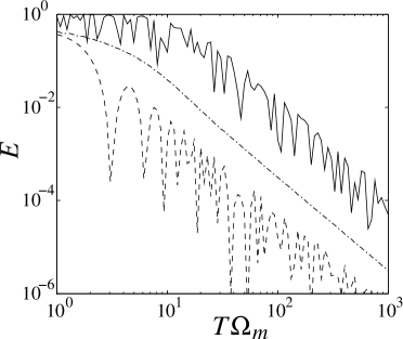
Figure 2: Log-log plot of the gate error, $E=1-{\cal F}$, for the Hadamard (solid), phase (dashed) and CNOT (dotted) gates, when we use the ideal Hamiltonians (7) and (8) to simulate them. The parameters for the simulations are $\{\Delta_{m}/\Omega_{m}=\tilde{\Delta}_{m}/\Omega_{m}=1/10,\varphi_{m}=\pi/4\}$, and we change the speed of the process to study the influence of non–adiabaticity.

4 Control of errors

In this section we study whether it is feasible to apply the methods developed in §3 to the physical setup envisioned in §2. First of all we will study how fast the operations from §3 must be performed in order to minimize the deviations from the adiabatic theorem. And second and most important, we have to consider contributions to the energy which escape the terms considered in equations (7) and (8). We will analyse both sources of error separately, combining analytical estimates with numerical simulations of our techniques for small number of atoms.

4.1 Adiabaticity

To study the sensitivity of our method against non–adiabatic processes, we have simulated the protocols (10)-(12) using the ideal model given by Hamiltonians (7) and (8). For each of the gates we have fixed all parameters $\{\Delta_{m}/\Omega_{m}=\tilde{\Delta}_{m}/\Omega_{m}=1/10,\varphi_{m}=\pi/4\}$ except the time, and then we have computed how the error decreases as we decrease the speed of the adiabatic passage. The results are shown in figure 2. As a figure of merit we have chosen the gate fidelity (M. A. Nielsen 2002)

$${\cal F}=2^{-n}|\mathrm{Tr}\{U_{ideal}^{\dagger}U_{real}\}|^{2}$$ (14)

where $n$ is the number of qubits involved in the gate, $U_{ideal}$ is the gate that we wish to produce and $U_{real}$ is the actual operation performed. As expected, the adiabatic theorem applies when the processes are performed with a sufficiently slow speed. Typically a time $T\sim 300/\Omega_{m}$ is required for the desired fidelity ${\cal F}=1-10^{-4}$.

It is also worth mentioning, that in figure 2 and 3, strong, rapid oscillations of the error are seen. These oscillations are due to either the nonadiabaticity of the process (figure 2), or to imperfections in the Hamiltonian (figure 3). For a two-level system undergoing adiabatic evolution it is easy to prove that, while the amplitude of the oscillations is proportional to the speed of the adiabatic process, the frequency is instead related to the energy difference between contiguous eigenspaces. This frequency is for us unknown, and consequently, these oscillations may not be used to improve the accuracy of our method by looking for some ‘magic times’.

4.2 Imperfections

Outside the non–adiabaticity of a real experiment, there are two other sources of error which we must consider. (i) The quotient $J_{b}/U_{bb}$ is nonzero, which means that more than one atom per well may be excited. (ii) Atoms in state $|{a}\rangle$ interact and hop. This introduces new terms in equation (3), which are of the form $J_{a,k}(a^{\dagger}_{k}a_{k+1}+a^{\dagger}_{k+1}a_{k})$, $U_{aa}a^{\dagger}_{k}a^{\dagger}_{k}a_{k}a_{k}$, and $U_{ab}a^{\dagger}_{k}b^{\dagger}_{k}a_{k}b_{k}$. And finally, (iii) atoms in either state may jump to neighbouring sites, permanently changing the occupation numbers.

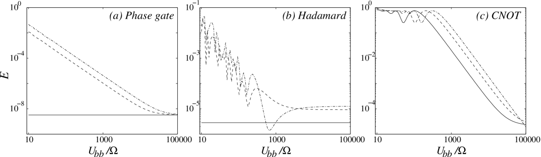
Figure 3: Log-log plot of the gate error, $E=1-{\cal F}$, for the (a) phase, (b) Hadamard and (c) CNOT gates. The parameters for the simulations are $U_{aa}=U_{ab}=J_{m}$, $J_{a}=J_{b}$,$g=U_{bb}+U_{ab}/2$, and $T=100/\Omega_{m}$. For the local gates we choose $\Delta_{m}=6\Omega_{m}=1$, and for the nonlocal gate $\Omega_{m}=J_{m}^{2}/6$. For each simulation we choose different population imbalance ($|n-m|=0,1,2$ for solid, dashed and dotted lines), and change the interaction constant $U_{bb}$.

The effects (i) and (iii) are suppressed if the coupling between internal levels and the amplitude of hopping are both small compared to the energy gap between our computation space and the undesired excitations. In other words, we require

$$(\Omega/U_{bb})^{2}\ll 1\quad\mathrm{and}\quad(J_{a,k}/U_{bb})^{2}\ll 1.$$ (15)

To analyse the remaining errors we develop an effective Hamiltonian which contains (6) and (3) plus new terms ($J_{a},U_{ab},U_{aa}$) that we did not consider before. In equation (6), the virtual excitation of two atoms increments the parameter $\Delta$ by an unknown amount, $\Delta_{\mathrm{eff}}\sim\Delta+2\Omega^{2}n_{k}/(\Delta+U_{ab}-U_{bb})$. If

$$U_{ab}\ll U_{bb}\quad\mathrm{and}\quad\Omega^{2}n_{k}T/U_{bb}\ll 1,$$ (16)

this shift may be neglected. In the two-qubit gates the energy shifts are instead due to virtual hopping of all types of atoms, and they are also accompanied by the possibility of swapping both qubits ($|{01}\rangle\leftrightarrow|{10}\rangle$). Both contributions are of the order of $\max(J_{b},J_{a})^{2}/g^{2}\sim J^{2}/U_{bb}$, and for

$$J^{2}T/U_{bb}\ll 1$$ (17)

they also may be neglected.

To quantitatively determine the influence of these errors we have simulated the evolution of two atomic ensembles with an effective Hamiltonian which results of applying second order perturbation theory to equation (3), and which takes into account all important processes. The results are shown in figures 3. In these pictures we show the error of the gates for simulations in which all parameters are fixed, except for $U_{bb}$ and the occupation numbers of the wells. The first conclusion is that the stronger the interaction between atoms in state $|{b}\rangle$, the smaller the energy shifts. This was already evident from our analytical estimates, because all errors are proportional to $1/U_{bb}$. Typically, a ratio $U_{bb}=10^{4}U_{ab}$ is required to make ${\cal F}=1-10^{-4}$. Second, the larger the number of atoms per well, the poorer the fidelity of the local gates [Figure 3(a-b)]. And finally, as figure 3(c) shows, the population imbalance between wells influences very little the fidelity of the two-qubit gate.

5 Conclusions

In this work we have shown that it is possible to perform quantum computation with cold atoms in a tunable optical lattice. Our scheme is based on performing adiabatic passage with one-qubit (7) and two-qubit (8) Hamiltonians. With selected paths and appropriate timing, it is possible to perform a universal set of gates (Hadamard gate, phase gate and a CNOT). Thanks to the adiabatic passage, the proposal works even when the number of atoms per lattice is unknown or the constants in the governing Hamiltonians have large uncertainties. These procedures can not only be used for quantum computing but also for quantum simulation (E. Jané 2002), and the same ideas can also be applied to other setups like the micro-traps demonstrated in R. Dumke (2002).

- [1] Aharonov, D. & Ben-Or, M. 1999 Fault-Tolerant Quantum Computation With Constant Error Rate. In Proc. of the 29th annual ACM symposium on Theory of computing pp. 176-188. New York: ACM Press. (DOI 10.1145/258533.258579.)
- [2]
- [3] Duan, L.-M., Cirac, J. I. & Zoller, P. 2001 Geometric Manipulation of Trapped Ions for Quantum Computation. Science 292, 1695.
- [4]
- [5] Charron, E., Tiesinga, E., Mies, F. & Williams, C. 2002 Optimizing a Phase Gate Using Quantum Interference. Phys. Rev. Lett. 88, 077901. (DOI 10.1103/PhysRevLett.88.07790.)
- [6]
- [7] Duan, L.-M. & Guo, G. 1999 Suppressing environmental noise in quantum computation through pulse control. Phys. Lett. A261, 139-144.
- [8]
- [9] Dumke, R., Volk, M., Müther, T., Buchkremer, F. B. J., Birkl, G. & Ertmer, W. 2002 Micro-optical Realization of Arrays of Selectively Addressable Dipole Traps: A Scalable Configuration for Quantum Computation with Atomic Qubits. Phys. Rev. Lett. 89, 097903. (DOI 10.1103/PhysRevLett.89.09790.)
- [10]
- [11] Eckert, K., Mompart, J., Yi, X. X., Schliemann, J., Bruss, D., Birkl, D. & Lewenstein, M. 2002 Quantum computing in optical microtraps based on the motional states of neutral atoms. arXiv:quant-ph/0206096.
- [12]
- [13] Falci, G., Fazio, R., Palma, G. M., Siewert, J. & Vedral, V. 2000 Detection of geometric phases in superconducting nanocircuits. Nature 407, 355.
- [14]
- [15] Greiner, M., Mandel, O., Esslinger, T., Hänsch, T. W. & Bloch, I. 2002 Quantum phase transition from a superfluid to a Mott insulator in a gas of ultracold atoms. Nature 415, 39-42.
- [16]
- [17] Ionicioiu, R. & Zanardi, P. 2002 Quantum-information processing in bosonic lattices. Phys. Rev. A 66, 050301. (DOI 10.1103/PhysRevA.66.050301.)
- [18]
- [19] Jaksch, D., et al. 1998 Cold bosonic atoms in optical lattices. Phys. Rev. Lett. 81, 3108-3111. (DOI 10.1103/PhysRevLett.81.3108.)
- [20]
- [21] Jaksch, D., et al. 1999 Entanglement of atoms via cold controlled collisions. Phys. Rev. Lett. 82, 1975-1978.
- [22]
- [23] Jané, E., Vidal, G., Dür, W., Zoller, P. & Cirac, J. I. 2002 Simulation of quantum dynamics with quantum optical systems. arXiv:quant-ph/0207011.
- [24]
- [25] Jones, J. A., Vedral, V., Ekert, A. & Castagnoli, G. 2000 Geometric quantum computation using nuclear magnetic resonance. Nature 403, 869-571.
- [26]
- [27] Knill, E., Laflamme, R. & Zurek, W. H. 1998 Resilient Quantum Computation. Science 279, 342-345.
- [28]
- [29] Nielsen, M. A. & Chuang, I. L. Chuang 2002. Quantum Computation and Quantum Information. Cambridge: Cambridge Univ. Press.
- [30]
- [31] Pachos, J., Zanardi, P. & Rasetti, M. 2000 Non-Abelian Berry connections for quantum computatio. Phys. Rev. A 61, 010305(R). (DOI 10.1103/PhysRevA.61.010305.)
- [32]
- [33] Recati, A., Calarco, T., Zanardi, P., Cirac, J. I. & Zoller, P. 2002 Holonomic quantum computation with neutral atoms. arXiv:quant-ph/0204030.
- [34]
- [35] Shor, P. W. 1996 Proc. 35th Annual Symposium on Fundamentals of Computer Science, pp. 56. Los Alamitos: IEEE Press.
- [36]
- [37] Steane, A. M. 2002 Overhead and noise threshold of fault-tolerant quantum error correction. arXiv:quant-ph/0207119.
- [38]
- [39] Viola, L. & Lloyd, S. 1998 Dynamical suppression of decoherence in two-state quantum systems. Phys. Rev. A 58, 2733-2744. (DOI 10.1103/PhysRevA.58.2733.)
- [40]
- [41] Zanardi, P. & Rasetti, M. 1999 Holonomic quantum computation. Phys. Lett. A 264, 94-99.