Energy level statistics for models of coupled single-mode Bose-Einstein condensates

Abstract

We study the distribution of energy level spacings in two models describing coupled single-mode Bose-Einstein condensates. Both models have a fixed number of degrees of freedom, which is small compared to the number of interaction parameters, and is independent of the dimensionality of the Hilbert space. We find that the distribution follows a universal Poisson form independent of the choice of coupling parameters, which is indicative of the integrability of both models. These results complement those for integrable lattice models where the number of degrees of freedom increases with increasing dimensionality of the Hilbert space. Finally, we also show that for one model the inclusion of an additional interaction which breaks the integrability leads to a non-Poisson distribution.

The application of random matrix theory to problems in physics can be traced back to the studies of Wigner w1 ; w2 in relation to the energy spectra of complex nuclei. (For a recent survey of the current state of the subject we refer to fsv .) The mathematical formalism was largely provided by Dyson d , who determined that the energy level spacing distribution displays universal behaviour depending only on the symmetry of the Hamiltonian. (This is in contrast to the energy distribution, i.e. density of states, which is generically non-universal.)

In this Letter we study the energy level spacing distribution for two models of coupled single-mode Bose-Einstein condensates. Both of these models are integrable (i.e., there exists a set of mutually commuting operators, which includes the Hamiltonian, the number of which is equal to the number of degrees of freedom in the system). These models are also integrable in the sense of the Quantum Inverse Scattering Method (QISM) kbi based on the Yang-Baxter equation, as shown in zlgm . We find that the energy level spacing distribution follows the universal Poisson form $P(s)=\exp(-s)$, where $s$ is the dimensionless energy gap parameter. Such a distribution indicates a lack of correlation between the energy levels, leading to random clustering. It was argued by Berry and Tabor bt , based on a semi-classical approach, that a Poisson distribution holds for integrable systems when the number of degrees of freedom is greater than one. This result has been supported by many numerical studies on one-dimensional lattice models with many degrees of freedom, such as the Heisenberg model, the Hubbard model and the $t-J$ model (at supersymmetric coupling) pzbmm ; ha ; am . The integrability of these models results from the fact that each can be derived through the QISM.

Our study for models of Bose-Einstein condensates is motivated by two factors. The first stems from the fact that the models we will analyse are integrable for a relatively large number of independent coupling parameters. This is in contrast to one-dimensional lattice models where integrability generally imposes severe constraints on the coupling parameters. The second motivation is that these examples are models with low numbers of degrees of freedom acting in Hilbert spaces with arbitrarily large dimensions. In am it is claimed that the reason for an integrable system to show a Poisson distribution for the level spacing is there exists a basis independent of the parameters in which the Hamiltonian is diagonal since there are as many commuting operators as the size of the Hilbert space. Or as explained in fsza , if there are an infinite number of conservation laws, then each subspace defined by a given set of quantum numbers contains a single level. Since the Poisson distribution occurs for the eigenvalue level spacings in random diagonal matrices, it should therefore apply to integrable systems. However, such an argument relies on there existing a large number of constants of the motion comparable to the dimension of the Hilbert space. The findings we present here surprisingly indicate that that the result is true even for systems with a small number of degrees of freedom, and does not rely on a semi-classical limit as in bt .

The first model we analyse is the two-site Bose-Hubbard model which has been widely applied for the study of two coupled Bose-Einstein condensates leggett . The Hamiltonian is

$$H = U_{11}N_{1}^{2}+U_{12}N_{1}N_{2}+U_{22}N_{2}^{2}+\mu_{1}N_{1}+\mu_{2}N_{2}$$ (1)

$$~{}~{}~{}~{}~{}-\frac{{\cal E}_{J}}{2}(a_{1}^{\dagger}a_{2}+a_{2}^{\dagger}a_{1}),$$

where the operators $a_{i},\,a^{\dagger}_{i},\,N_{i}=a^{\dagger}_{i}a_{i},\,i=1,2$ are associated to two Heisenberg algebras with relations

$$[a_{i},\,a_{j}^{\dagger}]=\delta_{ij},~{}~{}~{}[a_{i},\,a_{j}]=[a^{\dagger}_{i},\,a^{\dagger}_{j}]=0.$$

The model describes Josephson tunneling between two condensates with tunneling strength ${{\cal E}_{J}}/{2}$, the parameters $U_{ij}$ are the amplitudes for $S$-wave scattering and $\mu_{i}$ are chemical potentials. The Hilbert space of states is given by the infinite-dimensional Fock space spanned by the vectors

$$\left|m,n\right>=(a_{1}^{\dagger})^{m}(a_{2}^{\dagger})^{n}\left|0\right>,~{}~{}~{}~{}~{}~{}~{}~{}m,\,n=0,1,2,....,\infty.$$ (2)

As each basis vector is uniquely determined by the quantum numbers $m,n,$ this model has two degrees of freedom. The Hamiltonian commutes with the total particle number $N=N_{1}+N_{2}$, so the existence of the two conserved quantities, $H$ and $N$, shows that the model is integrable.   

$U_{11}$ $U_{22}$ $U_{12}$ $\mu_{1}$ $\mu_{2}$ $\Omega$ $\blacktriangle$ $0.01$ $0.01$ $-0.02$ $0.01$ $-0.01$ $100$ $\blacksquare$ $2.0$ $2.0$ $-4.0$ $1.0$ $-1.0$ $1.0$ $\bullet$ $100$ $100$ $-200$ $10$ $-10$ $0.01$

Table 1: Choices of coupling parameters for the Hamiltonian (1) used to determine the density of states shown in Fig. 1.

In Ref. zlgm it was demonstrated that (1) can be derived through the QISM and solved exactly using the algebraic Bethe ansatz. Here we will solve the model in the spirit of the co-ordinate Bethe ansatz, which allows us to exploit the tridiagonal structure of the Hamiltonian. Letting

$$\left|\Psi\right>=\sum_{m=0}^{N}\alpha_{m}\left(a_{1}^{\dagger}\right)^{N-m}\left(a^{\dagger}_{2}\right)^{m}\left|0\right>$$ (3)

it is easily shown, by directly evaluating the action of (1) on (3), that $\left|\Psi\right>$ is an eigenstate of (1) provided the co-efficients $\alpha_{m}$ satisfy, for $m>0$, the recursion relation

$$\alpha_{m+1}=X_{m}\alpha_{m}+\frac{m-N-1}{m+1}\alpha_{m-1}$$ (4)

such that $\alpha_{1}=X_{0}\alpha_{0}$, $\alpha_{N+1}=0$ and $X_{m}$ is defined by

$$\frac{{\cal E}_{J}(m+1)X_{m}}{2}\equiv U_{11}N^{2}+(U_{11}+U_{22}-U_{12})m^{2}$$

$$~{}~{}~{}~{}~{}~{}~{}+(U_{12}-2U_{11})mN+\mu_{1}N+(\mu_{2}-\mu_{1})m-E$$

where $E$ is the energy eigenvalue. It is clear that $\alpha_{m}$ is a polynomial in $E$ of order $m$. The $N+1$ roots of the equation $\alpha_{N+1}=0$ gives the complete energy spectrum for the sector with $N$ particles. Following rktb we can reduce the second order relation (4) to a first order relation. Letting

$$\alpha_{m+1}=\alpha_{0}\prod_{j=0}^{m}X_{j}Y_{j}$$

with $Y_{0}=1$ and substituting into (4) leads us to

$$Y_{m}=1+\frac{(m-N-1)}{(m+1)X_{m}X_{m-1}}\frac{1}{Y_{m-1}}$$ (5)

showing that $Y_{m}$ admits a continued fraction expansion. This provides a convenient means to generate the polynomials $\alpha_{m}$. For a given root $E$ of $\alpha_{N+1}=0$, this value may be substituted into the terms $\alpha_{m},\,m=1,...,N$ which permits us to compute the corresponding eigenstate through (3) (although this is not necessary for our studies here).

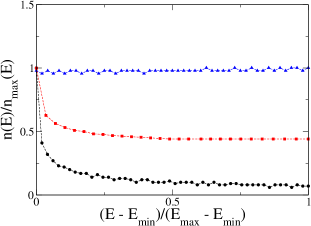
Figure 1: The density of states for the two-site Bose-Hubbard model with $1000$ particles, and interaction couplings given by Table I. The approximately constant profile in the case of the couplings ($\blacktriangle$) lying in the Rabi regime is reflective of the semi-classical nature of the pendulum analogy given in leggett . In contrast, for the couplings ($\bullet$) lying in the Fock regime the pendulum analogy is not semi-classical as indicated by a non-constant profile. The parameters ($\blacksquare$) within the Josephson regime illustrate the crossover behaviour, where the density of states deviates from the semi-classical profile at low energies.

For $U\sim U_{11}\sim U_{22}\sim-U_{12}/2$ it is common to divide the parameter space into three regimes leggett ; viz. Rabi ($U/{\cal E}_{J}<<N^{-1}$), Josephson ($N^{-1}<<U/{\cal E}_{J}<<N$) and Fock ($N<<U/{\cal E}_{J}$). There is a correspondence between (1) in these limits and the motion of a pendulum leggett . For both the Fock and Josephson regimes the analogy corresponds to a pendulum with fixed length, while in the Rabi regime the length varies. For both the Rabi and Josephson regimes the system is semi-classical. By semi-classical we intend that the energy per particle forms a continuum in the limit of large particle number. The Fock case is not semi-classical (e.g., there is a finite gap in the energy per particle between the ground and first excited state; see zlmg ,) and hence the argument of bt is not applicable. Fig. 1 shows the profile of the density of states $n(E)$, supporting this picture, with the coupling parameters for the Rabi, Josephson and Fock regimes given in Table I.

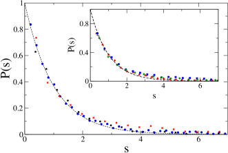
Figure 2: Energy level spacing distribution for the Bose-Hubbard model (1) in the sector $360\leq N\leq 400$, where the particle numbers are increased in units of 4. The total number of energy levels is 4,191. The distribution is independent of the choice of the coupling parameters, which are given by the first three columns of Table II. The inset shows the energy level spacing distribution for the remaining couplings given in Table II. The results show an excellent fit to the Poisson distribution $P(s)=\exp(-s)$, illustrated by the dashed curve in both the figure and inset.

To study the full level statistics of this model in the most general context is prohibitive because of the infinite dimensionality of the Hilbert space. It is important to emphasize that one cannot simply restrict to a sector of fixed particle number, as this has the effect that the restricted model has only one degree of freedom. In this instance, we have found that the Poisson distribution does not hold. As mentioned earlier, the Poisson distribution is only expected to hold when the numbers of degrees of freedom is greater than one. Therefore to investigate the level spacing statistics, we must conduct the analysis over a finite number of sectors with different particle number, in order to account for both degrees of freedom.   

$*$ $\bullet$ $\times$ $+$ $\blacktriangle$ $\blacksquare$ $\blacklozenge$ $U_{11}$ $0.01$ $2.0$ $100$ $3.1$ $-0.2$ $66.0$ $0.34$ $U_{22}$ $0.003$ $0.7$ $88$ $-0.14$ $0.4$ $28.0$ $3.45$ $U_{12}$ $0.0$ $0.0$ $0.0$ $0.001$ $10.0$ $0.3$ $0.0$ $\mu_{1}$ $0.0$ $0.0$ $0.0$ $15.0$ $0.0$ $3.14$ $0.12$ $\mu_{2}$ $0.0$ $0.0$ $0.0$ $-2.0$ $4.67$ $143$ $0.11$ $\Omega$ $100$ $1.0$ $0.01$ $0.5$ $10.0$ $0.24$ $15$

Table 2: Choices of coupling parameters for the Hamiltonian (1) used in Fig. 2.

We take subspaces of the Hilbert space comprised of sectors with fixed particle number $N$ (each of dimension $N+1$), starting at $N=360$, increasing in steps of 4 particles, up to $N=400$. This gives a total number of 4,191 energy levels. We calculate these energy levels for the wide range of coupling parameters given in Table II. While the first three choices for the coupling parameters in Table II correspond to the Rabi, Josephson and Fock regimes, the remaining values were chosen randomly. Note that we have deliberately not taken $U_{11}=U_{22}$ and $\mu_{1}=\mu_{2}$ in all cases since this corresponds to a discrete symmetry upon interchange of labels 1 and 2, leading to eigenvalue degeneracies which slightly complicates the analysis of the level spacing distribution.   

$*$ $\bullet$ $\times$ $+$ $\blacktriangle$ $\blacksquare$ $\blacktriangledown$ $\blacklozenge$ $U_{aa}$ $0.1$ $1.618$ $1.0$ $1.0$ $0.018$ $2.0$ $0.0$ $22.145$ $U_{bb}$ $0.1$ $1.618$ $1.0$ $-3.0$ $-0.82$ $-19.95$ $-1.0$ $4.0$ $U_{cc}$ $0.1$ $1.618$ $1.0$ $15.0$ $9.55$ $0.0$ $12.0$ $0.3$ $U_{ab}$ $0.1$ $1.618$ $1.0$ $-1.0$ $0.23$ $10.0$ $40.0$ $-2.29$ $U_{ac}$ $0.1$ $1.618$ $1.0$ $0.5$ $0.0$ $0.01$ $30.0$ $-36.9$ $U_{bc}$ $0.1$ $1.618$ $1.0$ $15.0$ $15.0$ $-3.0$ $-2.0$ $0.91$ $\mu_{a}$ $0.0$ $1.618$ $0.0$ $1.0$ $0.4447$ $0.0$ $-15.0$ $-2.0$ $\mu_{b}$ $0.0$ $1.618$ $0.0$ $-1.0$ $-0.61$ $-5.0$ $-28.0$ $5.0$ $\mu_{c}$ $0.0$ $1.618$ $0.0$ $-5.0$ $0.8939$ $1.3$ $-4.0$ $10.34$ $\Omega$ $100.0$ $1.618$ $0.001$ $10.0$ $-8.0$ $0.1$ $127$ $13.7$

Table 3: Choices of coupling parameters for the Hamiltonian (6) used in Fig. 3 and Fig. 4.

In determining the energy level spacing distribution for Fig. 2 no unfolding of the raw data was undertaken, nor required, unlike other studies pzbmm ; ha ; am . In each case the energy gaps were normalised by the largest gap, and a histogram built using, on average, 45 bins. In some cases there were a small number of large gaps (of approximately two orders of magnitude larger) relative to the average gap, which were discarded. In all cases the number of discarded data points was less than $1\%$ of the total. The curve $y=\gamma\exp(-\beta s)$ was fitted to each of the data sets. Finally, each histogram was normalised by the factor $\gamma^{-1}$ and the dimensionless gap parameter $s$ was rescaled in each case by $\beta^{-1}$. The data shown in Fig. 2 exhibits an excellent agreement with the theoretical Poisson distribution.

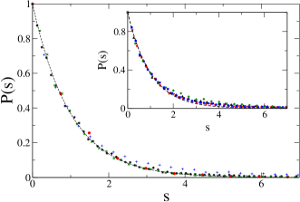
Figure 3: Energy level spacing distribution for the Hamiltonian (6) in the sector with $\mathcal{N}=400$ and $\mathcal{I}\geq 0$, which has $20,301$ energy levels. The coupling parameters are given by the first four columns of Table III, while the inset shows the data obtained for the remaining couplings in Table III. The distributions have universal behaviour independent of the choice of coupling parameters and follow the Poisson distribution $P(s)=\exp(-s)$, which is illustrated by the dashed curve in both the figure and the inset.

The model we analyse next is one for an atomic-molecular Bose-Einstein condensate with two distinct species of atoms, denoted $a$ and $b$, which can combine to produce a molecule $c$ zlgm . It also has an interpretation as a model for second harmonic generation in quantum optics wb where the non-linear terms in the number operators correspond to a Kerr non-linearity. The Hamiltonian takes the form

$$H_{0} = U_{aa}N_{a}^{2}+U_{bb}N_{b}^{2}+U_{cc}N_{c}^{2}$$ (6)

$$+U_{ab}N_{a}N_{b}+U_{ac}N_{a}N_{c}+U_{bc}N_{b}N_{c}$$

$$+\mu_{a}N_{a}+\mu_{b}N_{b}+\mu_{c}N_{c}+\Omega(a^{\dagger}b^{\dagger}c+c^{\dagger}ba)$$

which commutes with $\mathcal{I}=N_{a}-N_{b}$ and the total atomic number $\mathcal{N}=N_{a}+N_{b}+2N_{c}$. Along with $H_{0}$ this establishes that the model has three conserved integrals of motion.

The model acts on the infinite-dimensional Fock space spanned by the vectors

$$\left|l,m,n\right>=(a^{\dagger})^{l}(b^{\dagger})^{m}(c^{\dagger})^{n}\left|0\right>.$$ (7)

It is apparent that (6) has three degrees of freedom, specified by the quantum numbers $l,m,n$ in (7), and is thus integrable. For this model we can fix the total atomic number $\mathcal{N}$ and make the restriction $\mathcal{I}\geq 0$, which gives a Hamiltonian with two degrees of freedom acting in a finite Hilbert space of dimension $d=(\mathcal{N}^{2}+4\mathcal{N}+3)/8$ for $\mathcal{N}$ odd and $d=(\mathcal{N}^{2}+6\mathcal{N}+8)/8$ for $\mathcal{N}$ even.

The method described earlier for diagonalising (1) generalises in a straightforward way to (6). Using this method we have diagonalised (6) in the sector with $\mathcal{N}=400$ and $\mathcal{I}\geq 0$ (this gives a total of 20,301 energy levels) for the choice of couplings in Table III, and determined the energy level spacing distribution in exactly the same manner as described for (1). The results depicted in Fig. 3 indicate a Poisson distribution for the level spacings which is independent of the choice of coupling parameters.

Finally, we also examined the energy level spacings in the non-integrable Hamiltonian

$$\mathcal{H}=H_{0}+H_{1}$$ (8)

where $H_{1}=a^{\dagger}b+b^{\dagger}a$. Note that the presence of the term $H_{1}$ means that $\mathcal{H}$ commutes with $\mathcal{N}$, but does commute with $\mathcal{I}$. Each sector with fixed $\mathcal{N}$ has dimension $d=(\mathcal{N}^{2}+4\mathcal{N}+3)/4$ for $\mathcal{N}$ odd and $d=(\mathcal{N}^{2}+4\mathcal{N}+4)/4$ for $\mathcal{N}$ even. The results shown in Fig. 4 indicate that in this non-integrable case the level spacing distribution no longer fits the Poisson distribution, but lies closer to the Wigner surmise

$$P(s)=\frac{\pi s}{2}\exp\left(\frac{-\pi s^{2}}{4}\right),$$ (9)

which is the distribution for the Gaussian Orthogonal Ensemble (GOE) as expected for non-integrable time-reversal invariant Hamiltonians. A distinguishing feature of the GOE is level repulsion, which was well illustrated by Dyson d who showed an analogy between the distributions for the level spacings of the GOE and a system of unit charges, with Coulomb repulsion, confined to the unit circle in two dimensions.   

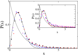
Figure 4: Energy level spacing distribution for the Hamiltonian (8) in the sector $50\leq\mathcal{N}\leq 100$, where the particle numbers are increased in units of 10. This gives a total of 9,331 energy levels. The choice of coupling parameters is given by the first four columns of Table II, while the inset shows the level spacing distribution for the remaining coupling parameters. The results show a good fit to the Wigner surmise (9) for a GOE distribution, which is indicated by the long-dashed curve (the short-dashed curve shows the Poisson distribution).

In conclusion, we have shown that two integrable models for systems of Bose-Einstein condensates exhibit universal Poissonian behaviour for the distribution of energy level spacings independent of the coupling parameters of the Hamiltonians. Both models provide examples with a low number of degrees of freedom acting in an arbitrarily large dimensional Hilbert space of states. To our knowledge this is the first study of this type and complements previous studies pzbmm ; ha ; am of level spacing distributions in integrable one-dimensional lattice models. For lattice models the number of degrees of freedom increases with increasing lattice length, and hence increasing dimensionality of the Hilbert space. Our results support the view that all integrable quantum systems show a Poisson distribution for the energy level spacings, indicative of clustering due to randomness, provided the number of degrees of freedom is greater than one bt . Our analysis also shows that this result does not rely on the existence of a semi-classical limit, as it holds for cases where the non-linear interactions dominate, such as for the Fock regime of (1). We have also studied a non-integrable example and shown that for this case the Poisson distribution no longer holds, and level repulsion is displayed. However, it is important to stress that the converse is not true: examples of quantum systems not exhibiting level repulsion, which are nonetheless classically non-integrable, have been shown to exist in bss . (We thank Peter Lévay for bringing this to our attention. See also kd .)

This work was supported by the Australian Research Council. We thank M.V. Berry and G.J. Milburn for helpful comments. S.R. Dahmen thanks The University of Queensland for generous hospitality.

References

- (1) E.P. Wigner, Proc. Camb. Phil. Soc. 47 790 (1951).
- (2) E.P. Wigner, Ann. Math. 62 548 (1955).
- (3) P.J. Forrester, N.C. Snaith and J.J.M. Verbaarschot, J. Phys. A: Math. Gen. 36 R1 (2003).
- (4) F.J. Dyson, J. Math. Phys. 3 140, 157, 166 (1962).
- (5) V.E. Korepin, N.M. Bogoliubov and A.G. Izergin, Quantum Inverse Scattering Method and Correlation Functions (Cambridge: Cambridge University Press 1993).
- (6) H.-Q. Zhou, J. Links, M.D. Gould and R.H. McKenzie, J. Math. Phys. 44 4690 (2003); J. Links, H.-Q. Zhou, R.H. McKenzie and M.D. Gould, J. Phys. A: Math. Gen. 36 R63 (2003).
- (7) M.V. Berry and M. Tabor, Proc. R. Soc. Lond. A 356 375 (1977).
- (8) D. Poilblanc, T. Ziman, J. Bellissard, F. Mila and G. Montambaux, Europhys. Lett. 22 537 (1993).
- (9) T.C. Hsu and J.-C. Anglès d’Auriac, Phys. Rev. B 47 14291 (1993).
- (10) J.-C. Anglès d’Auriac and J.-M. Maillard, Physica A 321 325 (2003) and refs. therein.
- (11) M. Faas, B.D. Simons, X. Zotos and B.L. Altshuler, Phys. Rev. B 48 5439 (1993).
- (12) A.J. Leggett, Rev. Mod. Phys. 73 307 (2001).
- (13) H.-Q. Zhou, J. Links, R.H. McKenzie and X.-W. Guan, J. Phys. A: Math. Gen. 36 L113 (2003).
- (14) A. Rybin, G. Kastelewicz, J. Timonen and N. Bogoliubov, J. Phys. A: Math. Gen. 31 4705 (1998).
- (15) D.F. Walls and R. Barakat, Phys. Rev. A 1 446 (1970).
- (16) J. Bolte, G. Steil and F. Steiner, Phys. Rev. Lett. 69 2188 (1992).
- (17) K. Kudo and T. Deguchi, Phys. Rev. B 68 052510 (2003).