Creating excitonic entanglement in quantum dots through the optical Stark effect

Abstract

We show that two initially non-resonant quantum dots may be brought into resonance by the application of a single detuned laser. This allows for control of the inter-dot interactions and the generation of highly entangled excitonic states on the picosecond timescale. Along with arbitrary single qubit manipulations, this system would be sufficient for the demonstration of a prototype excitonic quantum computer.

Semiconductor quantum dots (QD’s) are often described as ‘artificial atoms’ due to the discrete energy level structure which results from their three-dimensional confinement Jacak et al. (1998). Consequently, many of the techniques of quantum optics are now being used in QD studies and have led to the observation of Rabi oscillations Stievater et al. (2001), photon antibunching Michler et al. (2000), and recently the optical Stark effect Unold et al. (2004) in single QD’s. Such experiments have stimulated a great deal of interest in possible applications of QD’s in quantum information processing (QIP) devices Quiroga and Johnson (1999); Biolatti et al. (2002); Troiani et al. (2000).

In this paper, we shall analyze the behaviour of two adjacent self-assembled QD’s addressed by an external classical laser field, with the aim of controlling the electronic interactions between them. We shall demonstrate that it is possible to generate and maintain long-lived entangled excitonic states in such QD’s through the inter-dot resonant (Förster) energy transfer Lovett et al. (2003); Quiroga and Johnson (1999). This is achieved with a single laser that dynamically Stark shifts the exciton ground states in and out of resonance, effectively switching the inter-dot interaction on and off.

Our model considers only the ground state (no exciton) and first excited state (single exciton) in each dot, and these two states define our qubit as $|0\rangle$ and $|1\rangle$ respectively. Each QD is assumed to be within the strong-confinement regime where their typical sizes are much smaller than the corresponding bulk exciton radius, which is determined by the electron-hole Coulomb interaction. As a result, the confinement energy due to QD size dominates and mixing of the single-particle electron and hole states due to their Coulomb interactions may be neglected Schmitt-Rink et al. (1987). Any associated energy shift can be absorbed into the exciton creation energy; this shift is important as it ensures that the resonance condition for single-particle tunneling is not the same as that for resonant exciton transfer. Additionally, we consider only weak inter-dot interaction strengths ($\sim 0.1$ meV) which would be expected for two dots with relatively large spacing ($\sim 10$ nm) Nazir et al. . Therefore, we may neglect inter-dot tunneling of electrons and holes.

The Hamiltonian for two coupled dots in the presence of a single laser of frequency $\omega_{l}$ may be written in the computational basis $\{|00\rangle,|01\rangle,|10\rangle,|11\rangle\}$ as ($\hbar=1$):

$$H(t)=\left(\begin{array}[]{cccc}\omega_{0}&\Omega_{2}\cos{\omega_{l}t}&\Omega_{1}\cos{\omega_{l}t}&0\\ \Omega_{2}\cos{\omega_{l}t}&\omega_{0}+\omega_{2}&V_{\rm{F}}&\Omega_{1}\cos{\omega_{l}t}\\ \Omega_{1}\cos{\omega_{l}t}&V_{\rm{F}}&\omega_{0}+\omega_{1}&\Omega_{2}\cos{\omega_{l}t}\\ 0&\Omega_{1}\cos{\omega_{l}t}&\Omega_{2}\cos{\omega_{l}t}&\omega_{\rm T}+V_{\rm XX}\\ \end{array}\right),$$ (1)

where $\omega_{0}$ is the ground state energy, $\omega_{1(2)}$ the exciton creation energy for dot $1(2)$, and $\omega_{\rm T}=\omega_{0}+\omega_{1}+\omega_{2}$. The coupling terms $V_{\rm{F}}$ and $V_{\rm XX}$ are the Förster (transition dipole-dipole) and biexciton Troiani et al. (2000); Biolatti et al. (2002) (static dipole-dipole) interaction strengths respectively.

We have assumed that each dot may couple to the laser with a different strength, governed by the respective Rabi frequency $\Omega_{1}$ or $\Omega_{2}$, with $\Omega_{i}(t)\equiv-2{\bf d}_{i}\cdot{\bf E}({\bf r},t)$, for $i=1,2$. Here, ${\bf d}_{i}$ is the inter-band ground state transition dipole moment for dot $i$, and ${\bf E}({\bf r},t)$ is the laser amplitude at time $t$ and position ${\bf r}$. Natural size and composition fluctuations in self-assembled dot samples (for example in InGaAs QD’s Eliseev et al. (2000)) lead to a large range of possible transition dipole moments for each dot. The size of the ground-state dipole mismatch (and related exciton energy difference) between two dots is an important factor in determining our ability to control their interactions.

We shall first analyze the Hamiltonian of Eq. 1 within the rotating wave approximation (RWA). This will allow us to derive approximate conditions governing the behaviour of the system, and elucidate the mechanism for controlling excitonic entanglement. Subsequently, we shall characterize the small corrections to these RWA solutions and perform a full numerical solution of $H(t)$.

Transforming Eq. 1 into a frame rotating with the laser frequency $\omega_{l}$ with respect to both qubits, we obtain (within the RWA):

$$H^{\prime}=\left(\begin{array}[]{cccc}0&\Omega_{2}/2&\Omega_{1}/2&0\\ \Omega_{2}/2&\delta_{2}&V_{\rm F}&\Omega_{1}/2\\ \Omega_{1}/2&V_{\rm F}&\delta_{1}&\Omega_{2}/2\\ 0&\Omega_{1}/2&\Omega_{2}/2&\delta_{1}+\delta_{2}+V_{\rm XX}\\ \end{array}\right),$$ (2)

where $\delta_{i}=\omega_{i}-\omega_{l}$ is the detuning of the laser from dot $i$, and an irrelevant constant has been subtracted from each term on the diagonal. In order to demonstrate control over the interaction $V_{\rm F}$ we would like to isolate the behaviour of the $\{|01\rangle,|10\rangle\}$ subspace in which it acts. We may proceed, utilizing degenerate perturbation theory, provided that the following conditions are satisfied:

$$|\delta_{1}-\delta_{2}|,~{}|V_{\rm F}|,~{}|\Omega_{i}/2|\ll min(|\delta_{i}|,~{}|\delta_{i}+V_{\rm XX}|).$$ (3)

In this case the three subspaces {$\left|01\right\rangle$,$\left|10\right\rangle$}, {$\left|00\right\rangle$}, and {$\left|11\right\rangle$} are decoupled and we can write an effective Hamiltonian for the $\{|01\rangle,|10\rangle\}$ subspace:

$$\left(\begin{array}[]{cc}\delta_{2}+\alpha\Omega_{2}^{\prime 2}-\beta\Omega_{1}^{\prime 2}&V_{\rm F}+\Omega_{1}^{\prime}\Omega_{2}^{\prime}(\alpha-\beta)\\ V_{\rm F}+\Omega_{1}^{\prime}\Omega_{2}^{\prime}(\alpha-\beta)&\delta_{1}+\alpha\Omega_{1}^{\prime 2}-\beta\Omega_{2}^{\prime 2}\\ \end{array}\right),$$ (4)

where $\alpha=1/\delta_{1}$, $\beta=1/(\delta_{2}+V_{\rm XX})$, and $\Omega_{i}^{\prime}=\Omega_{i}/2$.

As we may control both the detunings $\delta_{i}$ of the laser from the QD’s, and the Rabi frequencies $\Omega_{i}$, it is possible to controllably modify the dynamics within this subspace. As is shown in Fig. 1, two regimes are of particular interest. When the laser is off, the difference in diagonal elements can be much larger than the effective interaction strength if

$$\omega_{1}-\omega_{2}\gg V_{\rm F}.$$ (5)

In this case, the eigenstates of Eq. 4 approach the computational basis states $|01\rangle$ and $|10\rangle$, shown away from the anticrossing in Fig. 1, that would be expected for non-interacting dots.

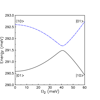
Figure 1: Laser induced anticrossing in the $\{|01\rangle,|10\rangle\}$ subspace, for fixed ratio $\Omega_{1}/\Omega_{2}=0.55$. Eigenvalues are calculated from Eq. 4 with $\delta_{1}=292.59$ meV, $\delta_{2}=290.59$ meV, and $V_{\rm F}=0.1$ meV.

In contrast, under the condition:

$$\delta_{1}-\delta_{2}=\omega_{1}-\omega_{2}=\left[\Omega_{2}^{\prime 2}-\Omega_{1}^{\prime 2}\right](\alpha+\beta),$$ (6)

the diagonal terms of Eq. 4 are equal and the two dots Stark shift into resonance under the action of the laser. The corresponding eigenstates lie at the anticrossing and are maximally entangled due to the modified off-diagonal interaction

$$V_{\rm eff}\equiv V_{\rm F}+\Omega_{1}^{\prime}\Omega_{2}^{\prime}(\alpha-\beta).$$ (7)

They are given by $|\psi_{+}\rangle=2^{-1/2}(|01\rangle+|10\rangle)$ and $|\psi_{-}\rangle=2^{-1/2}(|10\rangle-|01\rangle)$. Hence, if the system is initialized in the state $|01\rangle$, it will coherently evolve to $i|10\rangle$ during the laser pulse, passing through the maximally entangled state $2^{-1/2}(|01\rangle+i|10\rangle)$. This happens with a coherent exciton transfer time of $t=\pi/(2V_{\rm eff})$.

Therefore, we may selectively couple the two initially non-resonant QD’s (satisfying Eq. 5 before the laser is switched on) by the application of a single detuned laser satisfying Eq. 6 which non-adiabatically shifts the eigenstates to the anticrossing point in Fig. 1. As soon as we wish to decouple the dots again, we simply turn the laser off.

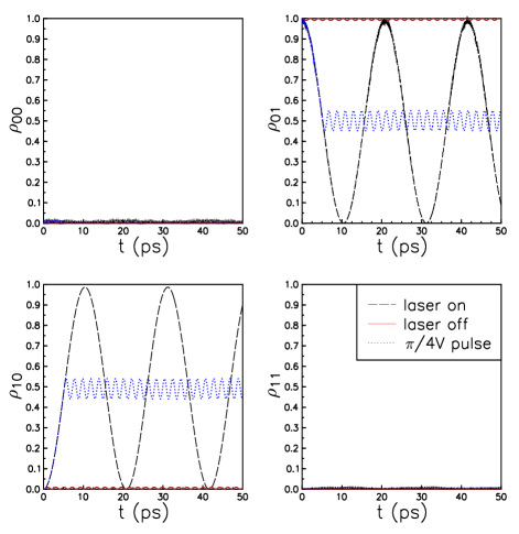
Figure 2: Populations of the four states $\left|00\right\rangle,\left|01\right\rangle,\left|11\right\rangle$ and $\left|10\right\rangle$ calculated from Eq. 2 with input $|01\rangle$, $\rho_{nm}=\langle nm|\rho|nm\rangle$, $V_{\rm F}=0.1$ meV and $V_{\rm XX}=0$. Dashed line: state evolution when the laser is always on. The Rabi frequencies and detunings of the laser are given by $\Omega_{2}~{}=~{}40.96$ meV, $\Omega_{1}=0.55\Omega_{2}$, $\Omega_{2}/2\delta_{1}=0.07$, and $\delta_{1}-\delta_{2}=2$ meV. Dotted line: state evolution when the same laser is on for a time of $\pi/(4V_{\rm eff})$ and then turned off. The small oscillations in population in the $\pi/(4V_{\rm eff})$ pulse case after the laser is switched off are due to some residual coupling between the dots which can be suppressed by increasing the energy selectivity $\delta_{1}-\delta_{2}$. Solid line: state evolution when the laser is always off. In this case the state is almost purely $\left|01\right\rangle$ throughout.

This effect is demonstrated in Fig. 2 where a numerical simulation of the evolution of an input state $|01\rangle$ under the RWA Hamiltonian of Eq. 2 is shown. Without laser coupling, the system remains in its initial state $|01\rangle$ with a fidelity, ${\cal F}>1-4\left(V_{\rm F}/|\delta_{1}-\delta_{2}|\right)^{2}=0.99$. However, under the application of a laser satisfying Eq. 6, coherent oscillations are observed between the states $|01\rangle$ and $|10\rangle$ with an exciton transfer time of $10.9$ ps, for the parameters chosen here. This transfer is very close to being $100\%$ complete with little population leaking from the $\{|01\rangle,|10\rangle\}$ subspace, justifying our perturbative treatment.

This behaviour could be observed in an experiment by applying a laser pulse for a series of different pulse lengths, and afterwards observing the emitted photons. As can be seen in Fig. 1, the two eigenstates when the laser is off (which are approximately $\left|10\right\rangle$ and $\left|01\right\rangle$) are separated by some 2 meV. This is readily resolved in a modern spectrometer – and so a measurement of the wavelength of the emitted photons can be use to determine which of the two dots each one came from. Plotting the number of each wavelength of detected photons as a function of the pulse length would allow a determination of the coherent transfer oscillations. Further, a $t=\pi/(4V_{\rm eff})$ pulse will create and maintain an (approximately maximally) entangled state from an initially separable one, and this is also shown in Fig 2. Even for the small coupling strength ($V_{\rm F}=0.1$ meV) considered here this operation is on the picosecond time scale. Therefore, we would expect such an entangled state to be long-lived in a pair of QD’s relative to the timescale of its generation. Single and coupled dot exciton lifetimes have been measured to be as long as nanoseconds at low temperatures Bayer and Forchel (2002); Birkedal et al. (2001); Borri et al. (2003). Additionally, pure phonon dephasing effects are suppressed as the temperature is lowered below 10 K Bayer and Forchel (2002); Borri et al. (2001).

We therefore now account for the finite exciton lifetimes by including only spontaneous emission terms in the density matrix master equation Agarwal (1974), and neglecting pure dephasing processes:

$$\dot{\rho}=-i[H,\rho]+\frac{1}{2}\sum_{i}\Gamma_{i}\left(2\sigma_{i}^{-}\rho\sigma_{i}^{+}-\sigma_{i}^{+}\sigma_{i}^{-}\rho-\rho\sigma_{i}^{+}\sigma_{i}^{-}\right).$$ (8)

Here, the $i$ label the dipole allowed transitions in the coupled system, $\sigma_{i}^{+}$ and $\sigma_{i}^{-}$ are their raising and lowering operators, and the $\Gamma_{i}$ are their transition rates. These terms can lead to a significant reduction of the degree of entanglement over time. We can see this by referring to Fig. 3, where we show the result of numerical calculations which use the full Hamiltonian (Eq. 1) in the master equation (Eq. 8). In Fig. 3 (a) the populations of the four states are shown as a function of time for the input state $|01\rangle$, subject to a square pulse of $5.45$ ps duration (this satisfies $t=\pi/(4V_{\rm eff})$ for our chosen parameters), and subject to significant decay. In Fig. 3 (b), we plot the entanglement of formation (EOF) Bennett et al. (1996) of the system as a function of time for the input state $|01\rangle$, for a variety of decay rates.

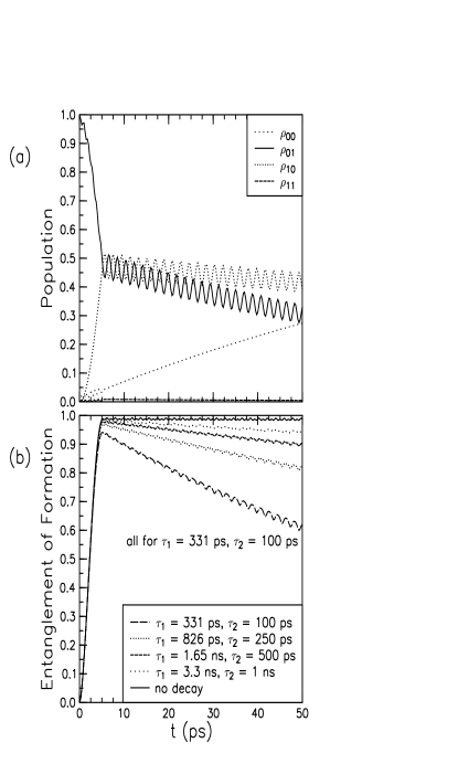
Figure 3: (a) Numerical simulation of the four populations for an input state $\left|01\right\rangle$ and a $\pi/(4V_{\rm eff})$ pulse. The simulation uses Eq. 8, which does not rely on the RWA and includes exciton decay, but not pure dephasing. The decay rates for dots $1$ and $2$ are given by $\Gamma_{1}=\tau_{1}^{-1}=(331~{}{\rm ps})^{-1}$ and $\Gamma_{2}=\tau_{2}^{-1}=(100~{}{\rm ps})^{-1}$ respectively. All other parameters are the same as for Fig. 2 except $\delta_{1}-\delta_{2}=2.18$ meV to account for the extra shifts, and $\omega_{l}=1500$ meV. (b) Entanglement of formation of the input state $|01\rangle$ as a function of time for a $\pi/(4V_{\rm eff})$ laser pulse, and for a series of different decay rates. We keep a constant ratio of $\Gamma_{1}/\Gamma_{2}=|{\bf d}_{1}/{\bf d_{2}}|^{2}=(\Omega_{1}/\Omega_{2})^{2}$. The calculations are made by using Eqs. 8-10.

The EOF measures the number of Bell states required to create the state of interest; for a maximally entangled state it is equal to unity while for a separable state it is zero. For a general two qubit state it is given by the equation

$$E_{F}({\rho})=h\left(\frac{1+\sqrt{1-\tau}}{2}\right),$$ (9)

where $h(x)=-x\log_{2}(x)-(1-x)\log_{2}(1-x)$ is the Shannon entropy function. $\tau$ is the “tangle” or “concurrence” squared, which can be computed by using the equation:

$$\tau={\cal C}^{2}=\left[\max\{\lambda_{1}-\lambda_{2}-\lambda_{3}-\lambda_{4},0\}\right]^{2}.$$ (10)

Here the $\lambda$’s are the square roots of the eigenvalues, in decreasing order, of the matrix ${\rho}\tilde{{\rho}}={\rho}\;\sigma_{y}^{A}\otimes\sigma_{y}^{B}{\rho}^{*}\sigma_{y}^{A}\otimes\sigma_{y}^{B}$, where ${\rho}^{*}$ denotes the complex conjugation of ${\rho}$ in the computational basis $\left|00\right\rangle,\left|01\right\rangle,\left|10\right\rangle,\left|11\right\rangle$ Munro et al. (2001). In Fig. 3 we see that at the end of the laser pulse the state has become almost maximally entangled and, in the absence of decay, stays so once the laser is switched off (the small deviation from unity is due to the residual effect of the Förster coupling when the laser is off). When decay is included the EOF decreases over time, but for typical experimental lifetimes of 1 ns Bayer and Forchel (2002); Birkedal et al. (2001); Borri et al. (2003), it retains a value which is higher than 0.94 for times up to 50 ps Reichardt .

The numerical solution of Eq. 8 required for Fig. 3 has been computed without making use of the RWA. The behaviour of the system is exactly as expected from the RWA case, except for an extra small shift in the dot energies when the laser is on. This shift is the largest correction to the Stark shift in a perturbative expansion and arises from the counter-propagating terms in the state evolution which are discarded when the RWA is made Barnett and Radmore (1997). The corrections to the RWA can all be derived by following the method of Shirley Shirley (1965), who considers the case of a two-level system (which we label 0 and 1 and consider to have an energy separation of $\omega_{1}$) coupled by an oscillating field (of frequency $\omega_{l}$). He shows that this kind of problem can be mapped on to a time independent one by using Floquet’s theory to construct a Hamiltonian in an infinite dimensional Hilbert space given by

$$\left\langle\alpha n\right|{\cal H}_{F}\left|\beta m\right\rangle={\cal H}_{\alpha\beta}^{n-m}+n\omega\delta_{\alpha\beta}\delta_{nm}.$$ (11)

Here $\alpha,\beta\in\{0,1\}$ and the $n,m$ represent Fourier components of the state evolution. ${\cal H}^{n}_{\alpha\beta}$ is the Fourier component with frequency $n\omega$ of the oscillating Hamiltonian (which is only non-zero for $\alpha\neq\beta$). Shirley showed that the time evolution operator of the two-level system can be written as

$$U_{\beta\alpha}(t;t_{0})=\sum_{n}\left\langle\beta n\right|\exp[-i{\cal H}_{F}(t-t_{0})]\left|\alpha 0\right\rangle e^{in\omega t}.$$ (12)

He goes on to derive the Bloch-Siegert shift, which is important for resonant interactions between the two-level system and the oscillating field. However, we are interested in the off-resonant behaviour. In the absence of any interactions, our system will initially be in a state of the form $a\left|00\right\rangle+b\left|10\right\rangle$ (in the notation $\left|\alpha n\right\rangle$), and we can use the time evolution operator (Eq. 12) to determine the energy separation of the two (eigen)states, $\left|00\right\rangle$ and $\left|10\right\rangle$. We follow a similar procedure when the laser is switched on. In this case, if the laser is sufficiently detuned from resonance (i.e. if $\delta=(\omega_{1}-\omega_{l})\gg\Omega/2$, with $\Omega$ the laser-system coupling), the $\left|\alpha n\right\rangle$ are still approximate eigenstates and we can employ second order perturbation theory to obtain the energy shift in the separation of the two levels. We obtain:

$$\Delta=\frac{2\Omega^{\prime 2}}{\delta}+\frac{2\Omega^{\prime 2}}{(\delta+2\omega_{l})}$$ (13)

where, as before, $\Omega^{\prime}=\Omega/2$. The extra term represents a detuning from resonance by an amount $2\omega_{l}+\delta$, compared to the term with detuning $\delta$ which is usually the only one kept. For the relatively large detunings considered in our two dot model, they become non-negligible contributions to the Stark shifts for each dot, $i$, with a magnitude of $2\Omega_{i}^{\prime 2}/(2\omega_{l}+\delta_{i})$. Once we account for this extra shift, for example in this calculation by redefining the parameters $\delta_{1}$ and $\delta_{2}$ to include it, the system behaves exactly as expected from our earlier analysis of Eq. 4.

We now assess the feasibility of our method by examining the state-of-the-art in real systems. In our previous work Lovett et al. (2003), we predicted that the Förster transfer energy can be as large as about 1 meV in QD’s (corresponding to energy transfer times on the sub-picosecond timescale); we also showed how a static electric field can be applied to the dots to suppress the interaction and so lengthen the transfer time as required. In addition to this, experimental work has suggested that Förster transfer times can approach picoseconds in structurally optimized pairs of CdSe QD’s Crooker et al. (2002), and that these transfer times can be on the subpicosecond timescale in photosynthetic biomolecular systems Herek et al. (2002). Molecular systems could therefore provide an alternative route to experimental realization of the effects we have predicted here.

QD exciton - laser interaction strengths (which correspond to the Rabi frequency when the laser is resonant with the exciton) of a few meV have been attained in an experiment which measured the optical Stark shift in AlAs/GaAs heterostructures Unold et al. (2004). Further, an experiment which directly observed Rabi oscillations in a InGaAs/GaAs QD photodiode also measured a Rabi frequency of a similar magnitude Zrenner et al. (2002). However, these experiments were not designed to maximize the laser - exciton coupling strength, and so the value of 40 meV, which we used in our simulations, is not unrealistic.

The coherent exciton transfer process detailed in Fig. 2 is equivalent to the realization of iSWAP logic operations between the pair of excitonic qubits Schuch and Siewert (2003). Along with arbitrary single qubit rotations, this gate would be sufficient for a demonstration of a prototype excitonic quantum computer. Single qubit operations in our two qubit system may be achieved by using their frequency addressability. A laser resonantly tuned to either of the two dots will induce a Rabi oscillation in the dot to which it is tuned; in the language of Pauli spin matices this is a rotation around the $X$ axis of the Bloch sphere, and represents one of the two rotations which are required for arbitrary single qubit operations. The other could be obtained in a number of ways. For example a slightly detuned laser will cause the qubit state to move around another trajectory on the Bloch sphere. Alternatively, a higher level $\left|T\right\rangle$ (of energy $\omega_{T}$ relative to the $\left|0\right\rangle$) could be used. If this higher level has a different energy for each qubit, it could be resonantly excited from, say, the $\left|0\right\rangle$ state in only one of the two qubits by applying an appropriately tuned $\pi$ laser pulse. Leaving the system to evolve then for a time $\tau$ before using another $\pi$ pulse to deexcite it causes the $\left|0\right\rangle$ to pick up a phase of $\omega_{T}\tau$ relative to the $\left|1\right\rangle$. This $Z$ rotation is sufficient to complete the set required for universal quantum computing.

If the ratio of decoherence time to gate operation time in our system were large enough, full scale fault tolerant quantum computing (FTQC) Steane (2003) would be possible. It is well established that a ratio of around 1000 is good enough for FTQC, and recent estimates of this have been a low as 100 Reichardt . We have demonstrated that an entangling gate can be performed in real systems in around 5 ps, which is around 200 times shorter than the longest measurements of decoherence times Bayer and Forchel (2002). Hence, our proposed scheme could be carried out with a precision which is already on the limit required for FTQC; incremental improvements in either FTQC protocols or in experimental systems should enable the implementation of full quantum algorithms. The absolute speed at which gates can be carried out in our scheme also makes them ideal for smaller scale applications such as quantum repeaters Dür et al. (2003), which require much less stringent gate fidelities than full scale FTQC.

To summarize, we have shown that two non-resonant QD’s may be brought into resonance by the application of a single detuned laser which induces Stark shifts within each dot without significant population excitation. This in turn allows for control over the inter-dot interactions, and hence the generation of highly entangled states on the picosecond timescale. The conditions of Eqs. 3, 5, and 6 set the upper limits on the energy selectivity and, neglecting incoherent processes, the fidelity possible with a particular dot sample. The Förster strength $V_{\rm F}$ sets the interaction timescale. In general, as the magnitude and difference of the Rabi frequencies increases, and as $V_{\rm F}$ increases, so does the feasibility of the proposed idea. We believe that the means to demonstrate the effects outlined above already exist. Moreover, these types of experiments may prove invaluable in assessing the potential applicability of semiconductor QD’s for future QIP technologies.

AN and BWL are supported by EPSRC (BWL as part of the Foresight LINK Award “Nanoelectronics at the Quantum Edge,” GR/R66029, and the QIPIRC, GR/S82176). We thank T. P. Spiller, S. D. Barrett, and W. J. Munro for useful and stimulating discussions, and R. G. Beausoleil for providing numerical simulation code.

References

- Jacak et al. (1998) L. Jacak, P. Hawrylak, and A. Wojs, Quantum Dots (Springer-Verlag, Heidelberg, 1998).
- Stievater et al. (2001) T. H. Stievater, X. Li, D. G. Steel, D. Gammon, D. S. Katzer, D. Park, C. Piermarocchi, and L. J. Sham, Phys. Rev. Lett. 87, 133603 (2001).
- Michler et al. (2000) P. Michler, A. Imamoǧlu, M. D. Mason, P. J. Carson, G. F. Strouse, and S. K. Buratto, Nature 406, 968 (2000).
- Unold et al. (2004) T. Unold, K. Mueller, C. Lienau, T. Elsaesser, and A. D. Wieck, Phys. Rev. Lett. 92, 157401 (2004).
- Quiroga and Johnson (1999) L. Quiroga and N. F. Johnson, Phys. Rev. Lett. 83, 2270 (1999).
- Biolatti et al. (2002) E. Biolatti, I. D’Amico, P. Zanardi, and F. Rossi, Phys. Rev. B 65, 075306 (2002).
- Troiani et al. (2000) F. Troiani, U. Hohenester, and E. Molinari, Phys. Rev. B 62, 2263(R) (2000).
- Lovett et al. (2003) B. W. Lovett, J. H. Reina, A. Nazir, and G. A. D. Briggs, Phys. Rev. B 68, 205319 (2003).
- Schmitt-Rink et al. (1987) S. Schmitt-Rink, D. A. B. Miller, and D. S. Chemla, Phys. Rev. B 35, 8113 (1987).
- (10) A. Nazir, B. W. Lovett, S. D. Barrett, J. H. Reina, and G. A. D. Briggs, eprint xxx.lanl.gov/quant-ph/0309099.
- Eliseev et al. (2000) P. G. Eliseev, H. Li, A. Stintz, G. T. Lin, T. C. Newell, K. J. Malloy, and L. F. Lester, Appl. Phys. Lett. 77, 262 (2000).
- Bayer and Forchel (2002) M. Bayer and A. Forchel, Phys. Rev. B 65, 41308(R) (2002).
- Birkedal et al. (2001) D. Birkedal, K. Leosson, and J. M. Hvam, Phys. Rev. Lett. 87, 227401 (2001).
- Borri et al. (2003) P. Borri, W. Langbein, U. Woggon, M. Schwab, M. Bayer, S. Fafard, Z. Wasilewski, and P. Hawrylak, Phys. Rev. Lett. 91, 267401 (2003).
- Borri et al. (2001) P. Borri, W. Langbein, S. Schneider, U. Woggon, R. L. Sellin, D. Ouyang, and D. Bimberg, Phys. Rev. Lett. 87, 157401 (2001).
- Agarwal (1974) G. S. Agarwal, Quantum Optics (Springer, Berlin, 1974).
- Bennett et al. (1996) C. H. Bennett, D. P. DiVincenzo, J. A. Smolin, and W. K. Wootters, Phys. Rev. A 54, 3824 (1996).
- Munro et al. (2001) W. J. Munro, D. F. V. James, A. G. White, and P. G. Kwiat, Phys. Rev. A 64, 030302 (2001).
- (19) If or are used as the input states, throughout the subsequent evolution..
- Barnett and Radmore (1997) S. M. Barnett and P. M. Radmore, Methods in Theoretical Quantum Optics (Clarendon Press, Oxford, 1997).
- Shirley (1965) J. H. Shirley, Phys. Rev. 138, B979 (1965).
- Crooker et al. (2002) S. A. Crooker, J. A. Hollingsworth, S. Tretiak, and V. I. Klimov, Phys. Rev. Lett. 89, 186802 (2002).
- Herek et al. (2002) J. L. Herek, W. Wohlleben, R. J. Cogdell, D. Zeidler, and M. Motzkus, Nature 417, 533 (2002).
- Zrenner et al. (2002) A. Zrenner, E. Beham, S. Stuffer, F. Findeis, M. Bickler, and G. Abstreiter, Nature 418, 612 (2002).
- Schuch and Siewert (2003) N. Schuch and J. Siewert, Phys. Rev. A 67, 032301 (2003).
- Steane (2003) A. M. Steane, Phys. Rev. A 68, 042322 (2003).
- (27) B. W. Reichardt, eprint xxx.lanl.gov/quant-ph/0406025.
- Dür et al. (2003) W. Dür, H.-J. Briegel, J. I. Cirac, and P. Zoller, Phys. Rev. A 59, 169 (1999).