On Quantum Cellular Automata

Abstract

In recent work [1] by Schumacher and Werner was discussed an abstract algebraic approach to a model of reversible quantum cellular automata (CA) on a lattice. It was used special model of CA based on partitioning scheme and so there is a question about quantum CA derived from more general, standard model of classical CA. In present work is considered an approach to definition of a scheme with “history,” valid for quantization both irreversible and reversible classical CA directly using local transition rules. It is used language of vectors in Hilbert spaces instead of $C^{*}$-algebras, but results may be compared in some cases. Finally, the quantum lattice gases, quantum walk and “bots” are also discussed briefly.

Introduction

Let us denote Hilbert space of one cell of a quantum cellular (or lattice gas) automata as $\mathcal{H}_{\bullet}$, then it is possible to consider different models of construction of Hilbert space for whole quantum system. In [1] was used model with tensor product of different spaces depicted here schematically as

$$\begin{array}[]{ccccccc}&\vdots&&\vdots&&\vdots&\\ \cdots&\mathcal{H}_{\bullet}&\otimes&\mathcal{H}_{\bullet}&\otimes&\mathcal{H}_{\bullet}&\cdots\\ &\otimes&&\otimes&&\otimes\\ \cdots&\mathcal{H}_{\bullet}&\otimes&\mathcal{H}_{\bullet}&\otimes&\mathcal{H}_{\bullet}&\cdots\\ &\vdots&&\vdots&&\vdots&\\ \end{array},$$ (1)

and more abstract model with $C^{*}$-algebras like

$$\begin{array}[]{ccccccc}&\vdots&&\vdots&&\vdots&\\ \cdots&\mathcal{A}&\otimes&\mathcal{A}&\otimes&\mathcal{A}&\cdots\\ &\otimes&&\otimes&&\otimes\\ \cdots&\mathcal{A}&\otimes&\mathcal{A}&\otimes&\mathcal{A}&\cdots\\ &\vdots&&\vdots&&\vdots&\\ \end{array}.$$ (2)

It also quite shortly was mentioned other model in relation with quantum lattice gases and quantum walks [1, V.E]

$$\begin{array}[]{ccccccc}&\vdots&&\vdots&&\vdots&\\ \cdots&\mathcal{H}_{\bullet}&\oplus&\mathcal{H}_{\bullet}&\oplus&\mathcal{H}_{\bullet}&\cdots\\ &\oplus&&\oplus&&\oplus\\ \cdots&\mathcal{H}_{\bullet}&\oplus&\mathcal{H}_{\bullet}&\oplus&\mathcal{H}_{\bullet}&\cdots\\ &\vdots&&\vdots&&\vdots&\\ \end{array},$$ (3)

The model with tensor products Eq. (1) is more familiar in quantum computer science, than model with direct sum Eq. (3). In such a case the abstract algebraic approach Eq. (2) is formally approved, because in general case state of cell (or sublattice) of lattice Eq. (1) may be simply not defined as a vector in Hilbert space $\mathcal{H}_{\bullet}$, but algebra of observables (and state of $C^{*}$-algebra) for any cell(s) is always defined.

To avoid such a problem here is formally used model Eq. (1) with finite lattices to have correctly defined notion of state for whole system, but quantum gates as usually may be defined for arbitrary set of cells (sites). In Sec. 1 such a system is considered from point of view of usual theory of quantum computational networks. The approach is related with question: how to adopt model of general CA for quantum computers by using standard tools from theory of quantum algorithms.

On the other hand, the particular model Eq. (1) does not necessary produce appropriate scheme for description of real space-time processes. In Sec. 2 as an illustrative example of physical applications is discussed a “qubot” model of quantum lattice gas automata using both “additive” Eq. (3) and “multiplicative” Eq. (1) schemes.

1 Quantum Networks for Cellular Automata

1.1 Cellular Automata with “History”

Let us consider usual procedure of rewriting of a classical algorithm for a quantum computer, i.e., two-steps process:

1. To change irreversible classical function to reversible one using well known methods: “quantum function evaluation,” “history tape,” etc.

2. To rewrite reversible function, i.e., a transposition of a set, as a matrix of the transposition, i.e., the unitary matrix. In such a way it is possible to write action of the function for arbitrary superposition of states.

Here is important to recall, that general definition of classical cellular automata includes the time dimension (see Fig. 1) [3]

$$s_{i}^{(t+1)}=F\bigl{(}\mathop{\textstyle{\coprod}}\limits_{j\in\mathcal{E}_{i}}s_{j}^{(t)}\bigr{)},$$ (4)

where $s_{i}\in S$ space of states, $\mathcal{E}_{i}$ is “local environment” of index $i$, $\amalg$ is a vector (disjoint union) of states $s_{j}$ in the environment, and $F$ is local transition function $F:S^{k}\to S$. E.g., for simplest 1D cellular automata used in examples below $F:S^{3}\to S$

$$s_{i}^{(t+1)}=F(s_{i-1}^{(t)},s_{i}^{(t)},s_{i+1}^{(t)})$$ (5)

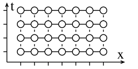
Fig. 1: Cellular automaton with time (history) dimension

Reversible analogue of Eq. (4) is map $\widetilde{F}:S^{k+1}\to S^{k+1}$, $\widetilde{F}^{-1}=\widetilde{F}$

$$\widetilde{F}\colon\Bigl{(}s_{i}^{(t+1)},\mathop{\textstyle{\coprod}}\limits_{j\in\mathcal{E}_{i}}s_{j}^{(t)}\Bigr{)}\mapsto\Bigl{(}F\bigl{(}\mathop{\textstyle{\coprod}}\limits_{j\in\mathcal{E}_{i}}s_{j}^{(t)}\bigr{)}\circleddash s_{i}^{(t+1)},\mathop{\textstyle{\coprod}}\limits_{j\in\mathcal{E}_{i}}s_{j}^{(t)}\Bigr{)}$$ (6)

where $\circleddash$ is some “subtracting” operation $S\times S\to S$, $a\circleddash 0=a$, $a\circleddash(a\circleddash b)=b$ like subtraction modulo $p$ for $S=\mathbb{Z}_{p}$ or “bitwise” XOR (addition modulo 2) for $S=\mathbb{Z}_{2}^{n}$ (see footnote (${}^{\ref{fn:qfe}}$) on page 2). For Eq. (5) map $\widetilde{F}:S^{4}\to S^{4}$ may be written as

$$\bigl{(}s_{i}^{(t+1)},s_{i-1}^{(t)},s_{i}^{(t)},s_{i+1}^{(t)}\bigr{)}\mapsto\bigl{(}F(s_{i-1}^{(t)},s_{i}^{(t)},s_{i+1}^{(t)})\circleddash s_{i}^{(t+1)},s_{i-1}^{(t)},s_{i}^{(t)},s_{i+1}^{(t)}\bigr{)},$$ (7)

It is clear, that reversible map $\widetilde{F}$ at each moment of $t$ acts on two adjacent “time layers” Fig. 3 and global transition function $\mathbf{\widetilde{F}}$ may be written as composition of all local $\widetilde{F}_{i}$

$$\mathbf{\widetilde{F}}=\mathop{\circledcirc}\limits_{i\in L}\widetilde{F}_{i}.$$ (8)

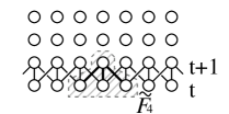
Fig. 2: Transition functions

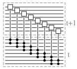
Fig. 3: Transition functions represented as network

So instead of one instance of lattice $L$ we have evolution with “generating a sequence of copies, history” as it is quite usual in theory of cellular automata [3], reversible classical [5], and quantum [6] computations.

1.2 Quantum Case

Let us now consider the quantum case. We have some lattice $L$ and each cell is described by Hilbert space $\mathcal{H}_{i}$, or $\mathcal{H}_{i}^{(t)}$ with explicit discrete time index

$$\mathcal{H}_{L}=\mathop{\textstyle{\bigotimes}}\limits_{i\in L}\mathcal{H}_{i},\quad\mathcal{H}_{L}^{(t)}=\mathop{\textstyle{\bigotimes}}\limits_{i\in L}\mathcal{H}_{i}^{(t)}.$$ (9)

Here is suggested that total Hilbert space of evolution may be represented as tensor product of Hilbert spaces $\mathcal{H}_{L}^{(t)}$ representing lattice for each time step.

$$\mathcal{H}_{\mathbb{T}}=\mathop{\textstyle{\bigotimes}}\limits_{t\in{\mathbb{T}}}\mathcal{H}^{(t)}_{L}$$ (10)

The reversible expression Eq. (6) may be represented for quantum case by some unitary operator $\hat{F}_{i}^{(t|t+1)}$ on space $\mathcal{H}_{\mathcal{E}_{i}}^{(t|t+1)}$

$$\hat{F}_{i}^{(t|t+1)}\colon\mathcal{H}_{\mathcal{E}_{i}}^{(t|t+1)}\to\mathcal{H}_{\mathcal{E}_{i}}^{(t|t+1)};\quad\mathcal{H}_{\mathcal{E}_{i}}^{(t|t+1)}=\mathcal{H}_{i}^{(t+1)}\otimes\bigl{(}\mathop{\textstyle{\bigotimes}}\limits_{j\in\mathcal{E}_{i}}\mathcal{H}_{j}^{(t)}\bigr{)},$$ (11)

expressed more directly as

$$\hat{F}_{i}^{(t|t+1)}=~{}\sum_{\hbox to0.0pt{$\scriptstyle s_{1},\dots,s_{k}\in S$\hss}}~{}\hat{f}^{(i,t+1)}_{s_{1},\dots,s_{k}}\otimes\hat{\mathsf{P}}_{s_{1}}^{(i_{1},t)}\otimes\cdots\otimes\hat{\mathsf{P}}_{s_{k}}^{(i_{k},t)},\quad\{i_{1},\dots,i_{k}\}\in\mathcal{E}_{i},$$ (12)

where $\hat{\mathsf{P}}_{s}$ are projectors, $\hat{f}$ are operators corresponding to local transition table representing $F$ of the cellular automata (say one of two $2\times 2$ matrices $\hat{\mathbf{1}}$ and $\hat{\sigma}_{x}$ in simplest case of $S=\mathbb{Z}_{2}$), and upper index $\hat{\cdot}^{(i,t)}$ of a “one-site” operator like $\hat{\mathsf{P}}$ or $\hat{f}$ corresponds to space-time coordinate $(x,t)$, see Fig. 1.

The global transition function $\hat{\mathbf{F}}^{(t\mapsto t+1)}$ may be represented as

$$\hat{\mathbf{F}}^{(t\mapsto t+1)}=\mathop{\textstyle{\prod}}\limits_{i\in L}\hat{F}_{i}^{(t|t+1)}.$$ (13)

The expression Eq. (13) is valid, because $\hat{F_{i}}$ commute despite of overlapping domains (see Fig. 3). It is more clear from representation of the global function $\hat{\mathbf{F}}$ as a quantum network Fig. 3 where $\hat{F}_{i}$ are “Controlled-F” gates and the commutativity may be checked by straightforward calculations using Eq. (12).

1.3 “Histories” Entanglement

The specific property of given model is entanglement between states at different times, see Eq. (20) below. It is related with some difference of considered scheme and alternative approach. Let us consider global transition rule

$$\hat{\mathbf{F}}^{(t\mapsto t+1)}\colon\mathcal{H}_{L}^{(t)}\otimes\mathcal{H}_{L}^{(t+1)}\to\mathcal{H}_{L}^{(t)}\otimes\mathcal{H}_{L}^{(t+1)}.$$ (14)

It has certain difference with “naíve evolution” approach

$$\hat{\mathbf{F}}_{e}^{(t\mapsto t+1)}\colon\mathcal{H}_{L}^{(t)}\to\mathcal{H}_{L}^{(t+1)}$$ (15)

or even

$$\hat{\mathbf{F}}_{e}\colon\mathcal{H}_{L}\to\mathcal{H}_{L}.$$ (16)

In the [1] is used Heisenberg picture instead of Schrödinger one used here, but all expressions used above may be simply rewritten in such a picture

$$\hat{A}\mapsto\hat{\mathbf{F}}\hat{A}\hat{\mathbf{F}}^{-1}$$ (17)

and it is clear, that in [1] is used approach with Eq. (16), but not with Eq. (14).

On the other hand, Eq. (15) or Eq. (16) may be rewritten in form Eq. (14) using special operator defined on basis elements as

$$\hat{\mathbf{F}}_{\mathsf{X}}\bigl{(}|K\rangle\otimes|R\rangle\bigr{)}=|R\rangle\otimes(\hat{\mathbf{F}}_{e}|K\rangle),\quad\hat{\mathbf{F}}_{\mathsf{X}}=\hat{{\mathsf{X}}}_{12}\circ(\mathbf{1}\otimes\hat{\mathbf{F}}_{e}),$$ (18)

where $\hat{{\mathsf{X}}}_{12}$ is “swap” operator.

It is suggested, that second space is “initialized” by some state $|0\rangle$, and it is clear that already for classical global transition function $\mathbf{F}$ we have two different schemes. The scheme discussed in present paper is defined on basic states as

$$\hat{\mathbf{F}}\colon|K\rangle\otimes|R\rangle\mapsto|K\rangle\otimes|\mathbf{F}(K)\circleddash R\rangle,\quad\hat{\mathbf{F}}\bigl{|}K,0\bigr{\rangle}=\bigl{|}K,\mathbf{F}(K)\bigr{\rangle}$$ (19)

and unitary both for reversible and irreversible global functions. Let us consider application of Eq. (19) to composition of two basic states of lattice

$$\hat{\mathbf{F}}\bigl{(}(\alpha|K_{1}\rangle+\beta|K_{2}\rangle)\otimes|0\rangle\bigr{)}=\alpha|K_{1}\rangle\otimes|\mathbf{F}(K_{1})\rangle+\beta|K_{2}\rangle\otimes|\mathbf{F}(K_{2})\rangle$$ (20)

The Eq. (20) describes entangled state if $\mathbf{F}(K_{1})\neq\mathbf{F}(K_{2})$, i.e., for reversible CA such states are always entangled and only for irreversible CA some compositions are evolving to non-entangled states.

Other scheme, Eq. (18)

$$\hat{\mathbf{F}}_{\mathsf{X}}\bigl{|}K,0\bigr{\rangle}=\bigl{|}0,\mathbf{F}_{e}(K)\bigr{\rangle}$$ (18^′)

unitary only for reversible global function. It is clear, that Eq. (18^′) never entangles two states

$$\hat{\mathbf{F}}_{\mathsf{X}}\bigl{(}(\alpha|K_{1}\rangle+\beta|K_{2}\rangle)\otimes|0\rangle\bigr{)}=|0\rangle\otimes\bigl{(}\alpha|\mathbf{F}(K_{1})\rangle+\beta|\mathbf{F}(K_{2})\rangle\bigr{)}$$ (21)

and so may be really modeled by simpler expression Eq. (16). On the other hand Eq. (19) entangles two terms, but for reversible function it may be disentangled using function

$$\hat{\mathbf{F}}^{\prime}\colon|K\rangle\otimes|R\rangle\mapsto|\mathbf{F}^{-1}(R)\circleddash K\rangle\otimes|R\rangle,$$ (22)

$$\hat{\mathbf{F}}^{\prime}\bigl{|}K,\mathbf{F}(K)\bigr{\rangle}=\bigl{|}0,\mathbf{F}(K)\bigr{\rangle}\quad\Rightarrow\quad\hat{\mathbf{F}}^{\prime}\bigl{(}\hat{\mathbf{F}}(|\psi\rangle|0\rangle)\bigr{)}=|0\rangle\bigl{(}\hat{\mathbf{F}}_{e}|\psi\rangle\bigr{)}.$$ (23)

1.4 Second-Order CA

Yet another interesting possibility — is to consider suggested model of cellular automata with cyclic time. For such a case it is also possible to rewrite Eq. (14) as Eq. (16) for some reversible CA. Let us consider for example simple case with two time steps Fig. 4 (here second term in Eq. (19) already is not always $|0\rangle$).

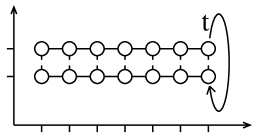
Fig. 4: Cyclic time condition (with two layers)

In such a case evolution Eq. (14) may be expressed in form Eq. (16) using new model with same lattice, but extended configuration space of each cell $\mathcal{H}^{\prime\prime}_{i}=\mathcal{H}_{i}\otimes\mathcal{H}_{i}$. In classical case it corresponds to well known “second-order” Fredkin scheme for construction of reversible cellular automaton from irreversible one using two consequent states of lattice for calculation of each step, similarly with some reversible second-order differential equations [3, 4].

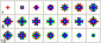
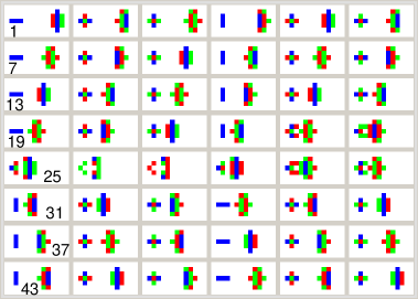
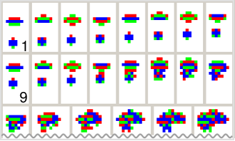
Fig. 5: “Reversible Game of Life” examples

On Fig. 5 is reproduced example of evolution of reversible classical CA produced by such a way from famous Conway’s “Game of Life” irreversible CA [7]. Methods described above let us consider action of such CA on arbitrary quantum superposition of basic states, and generalization to “quantum transition tables” is more or less straightforward, but outside of scope of this note.

It is also possible to use the same internal space, but double lattice $L\times L$, $\mathcal{H}_{L}\otimes\mathcal{H}_{L}\cong\mathcal{H}_{L\times L}$. Evolution is described by two steps, with second one is swap of two copies of lattice, but unlike [1] formal partitioning scheme used for such process Fig. 6 has overlapped partitions at first step ($F_{i}$, see also Fig. 3).

Fig. 6: Formal partitioning for Fig. 4

1.5 Two-Steps Partitioning

Scheme suggested above still does not include Margolus partitioning used in [1] and described as two-step process Fig. 8. More rigorously, Margolus scheme as particular example of definition Eq. (4) (with two different $F$ for odd and even moments of time) is valid for quantization of classical CA with transition function $F$, but does not have extension to quite straightforward generalization to quantum case with general unitary operator $\hat{{\mathcal{Q}}}$ applied to each subunit of partitioning (dashed ellipse in example with 1D cellular automaton on Fig. 8).

Fig. 7: Two-step partitioning

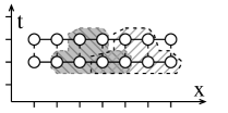
Fig. 8: Extended partitioning

The model needs for subtler construction. It is possible for example to consider extended $(t,t+1)$ neigbourhood (see Fig. 8) for local transition functions $\hat{F}_{i\times n}^{(t|t+1)}$ and use more difficult expression instead of Eq. (12).

Let us consider example with 1D cellular automata with Margolus partitioning and unitary transformation $\hat{{\mathcal{Q}}}:\mathcal{H}\otimes\mathcal{H}\to\mathcal{H}\otimes\mathcal{H}$ applied two times to different partitioning Fig. 8. Then local transition function $\hat{F}_{i\times 2}^{(t|t+1)}$ for both steps of the process using neighborhood with 6 ($4\to 2$) elements in two time layers is depicted on Fig. 8 and may be expressed as

$$\begin{split}&\hat{F}_{i\times 2}^{(t|t+1)}=\bigl{(}\hat{{\mathcal{Q}}}^{(\begin{subarray}{l}2i-1\\ 2i\end{subarray},\,t)}\otimes\hat{{\mathcal{Q}}}^{(\begin{subarray}{l}2i+1\\ 2i+2\end{subarray},\,t)}\bigr{)}^{\!-1}\hat{{\mathcal{Q}}}^{(\begin{subarray}{l}2i\\ 2i+1\end{subarray},\,t+1)}\hat{\complement}\!\mathtt{\symttup}\bigl{(}\hat{{\mathcal{Q}}}^{(\begin{subarray}{l}2i-1\\ 2i\end{subarray},\,t)}\otimes\hat{{\mathcal{Q}}}^{(\begin{subarray}{l}2i+1\\ 2i+2\end{subarray},\,t)}\bigr{)},\\ &\hat{\complement}\!\mathtt{\symttup}=\hat{\complement}^{(\begin{subarray}{l}2i\\ 2i+1\end{subarray},\,\begin{subarray}{l}t\\ t+1\end{subarray})}=\sum_{s_{1},s_{2}}(\hat{\mathsf{U}}^{(2i,t+1)})^{s_{1}}\otimes(\hat{\mathsf{U}}^{(2i+1,t+1)})^{s_{2}}\otimes\hat{\mathsf{P}}^{(2i,t)}_{s_{1}}\otimes\hat{\mathsf{P}}^{(2i+1,t)}_{s_{2}},\end{split}$$ (24)

where $\hat{\complement}\!\mathtt{\symttup}$ acts on basis elements as

$$\hat{\complement}\!\mathtt{\symttup}\colon\bigl{|}s_{1},s_{2}\bigr{\rangle}\otimes\bigl{|}0,0\bigr{\rangle}\mapsto\bigl{|}s_{1},s_{2}\bigr{\rangle}\otimes\bigl{|}s_{1},s_{2}\bigr{\rangle},$$ (25)

and $\hat{\mathsf{U}}$ in Eq. (24) is Weyl “cyclic shift” operator, $\hat{\mathsf{U}}:|s\rangle\mapsto|s+1\mod m\rangle$.

So at first $\hat{{\mathcal{Q}}}$ are applied to blocks $(2i-1,2i|t)$ and $(2i+1,2i+2|t)$, next, $\hat{\complement}\!\mathtt{\symttup}$ “spreads” block $(2i,2i+1)$ from $(t)$ to $(t+1)$, $\hat{{\mathcal{Q}}}$ is applied to block $(2i,2i+1|t+1)$ and, finally, first two applications of $\hat{{\mathcal{Q}}}$ to $(2i-1,\cdots,2i+2|t)$ are “undone”. The formula Eq. (24) let us check directly, that such operators $\hat{F}_{2\times i}^{(t|t+1)}$ for different “even neighborhoods” Fig. 8 are really commuting.

It should be mentioned, that such definition of transition function depends on choice of basis in Hilbert space, because definition of $\hat{\complement}\!\mathtt{\symttup}$ Eq. (25) depends on basis — in agreement with famous no-cloning theorem [8] only set of orthogonal states may be cloned perfectly. On the other hand, it may be simply checked that for change of basis in each cell described by unitary operator $\hat{\mathcal{B}}$ we formally simply may use the same definition of $\hat{F}_{i\times 2}^{(t|t+1)}$ with new function

$$\hat{{\mathcal{Q}}}^{\prime}=(\hat{\mathcal{B}}\otimes\hat{\mathcal{B}})\>\hat{{\mathcal{Q}}}\>(\hat{\mathcal{B}}^{*}\otimes\hat{\mathcal{B}}^{*}).$$ (26)

Furthermore, it is possible to consider new lattice with two-cells block of partitioning (at second time step) considered as new cell of lattice. Then we have new transition function $\hat{F}_{i}$ with “shape” Fig. 3 like Eq. (11), but expression more difficult than Eq. (12). Such observation let us suggest for definition of quantum cellular automata arbitrary set of local transition functions with only condition

$$\hat{F}_{i}^{(t|t+1)}\hat{F}_{j}^{(t|t+1)}=\hat{F}_{j}^{(t|t+1)}\hat{F}_{i}^{(t|t+1)},\quad[\hat{F}_{i}^{(t|t+1)},\hat{F}_{j}^{(t|t+1)}]=0,$$ (27)

or maybe even more general

$$\hat{F}_{i}^{(t|t+1)}\hat{F}_{j}^{(t|t+1)}=\omega_{i,j}\hat{F}_{j}^{(t|t+1)}\hat{F}_{i}^{(t|t+1)},\quad|\omega_{i,j}|=1,$$ (28)

because common complex phase does not change state and so global transition function represented as product Eq. (13) is correct for any ordering of $\hat{F}_{i}$.

1.6 Problem with Space-Time QCA Models

The model of QCA considered here may be realized using standard quantum network model, but in such a case the history is implemented not as time dimension, but as additional dimension of “hypercube network” necessary for “quantum function evaluation.” Is it possible to use such QCA as models of some physical processes in space-time?

Spacetime localised algebras was briefly discussed in [1, V.F]. With approach used in present paper construction of QCA used in [1] may be compared with a model of reversible CA “erasing their own history” via $\hat{\mathbf{F}^{\prime}}$ Eq. (23). If it is really necessary to perform such erasure, especially if to keep in mind possibility of applications to theory to irreversible CA? Moreover, in initial expression Eq. (4) for local classical transition rule there is no clear difference between reversible and irreversible case.

There is certain problem with covariance for QCA with space-time lattice as a model of physical events. Let us consider for example “lattice” with only one point and two states. How to model even trivial evolution with spreading without change? It is not possible to use map like

$$|\psi\rangle\underbrace{|0\rangle\cdots|0\rangle\!}_{T}\to|\psi\rangle|\psi\rangle\underbrace{|0\rangle\cdots|0\rangle\!}_{T-1}\to|\psi\rangle|\psi\rangle|\psi\rangle\underbrace{|0\rangle\cdots|0\rangle\!}_{T-2}\to\cdots,$$ (29)

unless $|\psi\rangle$ is not one of two fixed orthogonal states, as it was always in consideration above, because otherwise Eq. (29) describes nonlinear map, it is the subject of quantum no-cloning theorem [8].

Minor problem here is non-invariant state $|0\rangle^{\otimes T}$, because formally it may be corrected by addition of third, “empty (vacuum) state” $|\emptyset\rangle$, but it does not resolve main problem, because

$$|\psi\rangle|\emptyset\rangle^{\otimes T}\to|\psi\rangle|\psi\rangle|\emptyset\rangle^{\otimes T-1}\to|\psi\rangle|\psi\rangle|\psi\rangle|\emptyset\rangle^{\otimes T-2}\cdots$$ (29^′)

is nonlinear cloning anyway and so prohibited by quantum laws.

The problem is not only due to suggested approach, it was already mentioned, that “naíve evolution” model may be described in similar way. In such a case instead of Eq. (29) we would write

$$|\psi\rangle|0\rangle^{\otimes T}\to|0\rangle|\psi\rangle|0\rangle^{\otimes T-1}\to|0\rangle|0\rangle|\psi\rangle|0\rangle^{\otimes T-2}\cdots.$$ (30)

The Eq. (30) with “automata erasing own histories” is certainly linear, unitary, but it is not a picture we could expect for description of space-time model of real physical system.

Yet another idea is to use direct sum instead of tensor product for “joining” of state of lattice for different times

$$\mathcal{H}^{\oplus}_{\mathbb{T}}=\mathop{\textstyle{\bigoplus}}\limits_{t\in{\mathbb{T}}}\mathcal{H}^{(t)}_{L},$$ (31)

but it is not clear from very beginning, why we should distinguish time dimension by such a way, especially in applications for relativistic models.

Some clarification of the question may be based on application of quantum lattice gas automata (QLGA) model and discussed in Sec. 2.4. Simplest model of transition from QLGA to QCA is considered in Sec. 2.5. This example prompts yet another possible representation for one-particle trivial evolution as composition (up to normalization)

$$|\psi^{\mathbb{T}}\rangle=|\psi\rangle|0\rangle^{\otimes T}+|0\rangle|\psi\rangle|0\rangle^{\otimes T-1}+|0\rangle|0\rangle|\psi\rangle|0\rangle^{\otimes T-2}+\cdots,$$ (32)

but already for two particles trivial evolution, an expression may be rather cumbersome Eq. (52).

2 Quantum Lattice Gas Automata (QLGA)

From point of view of physical applications the theory of lattice gases [3, 4, 9, 10] devotes special attention. For short “translation” of some ideas of quantum field theory to language of quantum information science, here may be convenient to use following model.

2.1 Quantum ‘Bot’ on Lattice

The quantum bot or qubot [11] is quantum system with Hilbert space decomposed in natural way on two components:

$$\mathcal{H}_{\bot}=\mathcal{H}_{\ell}\otimes\mathcal{H}_{S},$$ (33)

there $\mathcal{H}_{\ell}$ corresponds to spatial degrees of freedom of lattice ($\dim\mathcal{H}_{\ell}=l=k^{D}$ for D-dimensional hypercubic lattice with $k$ cells in each side) and $\mathcal{H}_{S}$ — to internal states. It is the programmed quantum excitation, just approach with model Eq. (3), and also has analogue with quantum robots [12].

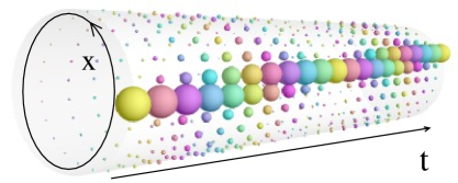
Fig. 9: Evolution of a qubot on cycle (size – amplitude, color – phase)

Evolution of qubot may be described by conditional quantum dynamics [13], a simple case with $\dim\mathcal{H}_{S}=2$ is

$$\hat{E}_{\bot}=\mathsf{U}\otimes|0\rangle\langle 0|+\mathsf{U}^{*}\otimes|1\rangle\langle 1|,$$ (34)

where $\mathsf{U}$ is Weyl shift operator, i.e., for internal state $|0\rangle$ or $|1\rangle\in\mathcal{H}_{S}$ Eq. (34) describes either left or right translation on the lattice $\mathcal{H}_{\ell}$. For simple expression Eq. (34) it is even possible to find Hamiltonian or consider “continuous time evolution” $\hat{E}_{\bot}^{\tau}$ [11], see Fig. 9.

So-called coined quantum walk (CQW) on cycle [14] may be described as composition of Eq. (34) and Hadamard transform applied to $\mathcal{H}_{S}$. Really it is not quite clear, if Hadamard CQW may be considered as “true quantum analogue” of classical random walk — it rather resembles superposition of two excitations (“qubots”) traveling in opposite directions. It is especially clear, if to choose new basis in $\mathcal{H}_{S}$, there Hadamard transform becomes diagonal. Such a note may be essential, e.g., quantum walk with proper correspondence with classical case has straightforward representation using infinite-dimensional internal space $\mathcal{H}_{S}$, but it should be discussed elsewhere. Furthermore, CQW is not only suggested model of quantum walk [15], and most likely it was discussed in [1, V.E] just due to the natural tie with lattice gas models.

2.2 Systems with Many Qubots

The total Hilbert space with $n$ equal qubots on a lattice may be described as symmetric product

$$\mathcal{H}_{\top^{n}}=\mathcal{H}_{\odot^{n}}=\mathop{\textstyle{\bigodot}}\limits_{i=1}^{n}\mathcal{H}_{\bot}$$ (35)

or as antisymmetric one

$$\mathcal{H}_{\top^{n}}=\mathcal{H}_{\wedge^{n}}=\mathop{\textstyle{\bigwedge}}\limits_{i=1}^{n}\mathcal{H}_{\bot}.$$ (36)

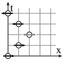
a) $\mathcal{H}_{\bot\mathnormal{1}}$

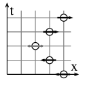
b) $\mathcal{H}_{\bot\mathnormal{2}}$

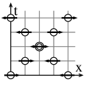
c) $\mathcal{H}_{\bot\mathnormal{1}}\odot\mathcal{H}_{\bot\mathnormal{2}}$

Fig. 10: Reversible QLGA (symmetric product)

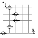
a) $\mathcal{H}_{\bot\mathnormal{1}}$

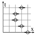
b) $\mathcal{H}_{\bot\mathnormal{2}}$

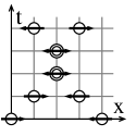
c) $\mathcal{H}_{\bot\mathnormal{1}}\otimes\mathcal{H}_{\bot\mathnormal{2}}$

Fig. 11: Reversible QLGA (tensor product)

Simpler expression with usual tensor product

$$\mathcal{H}_{\top^{n}}=\mathcal{H}_{\otimes^{n}}=\mathop{\textstyle{\bigotimes}}\limits_{i=1}^{n}\mathcal{H}_{\bot},$$ (37)

does not take into account quantum statistics and may be used for description of $n$ distinguishable qubots or as preliminary step for construction of more complicated expressions Eq. (35) and Eq. (36). It should me mentioned yet, that often quantum indistingushability principle may be essential. See for example Fig. 10, where at moment of collision of particles state of composite system is defined correctly Fig. 10(c), but state of each particular particle formally may be undefined Fig. 10(a,b). It is even does not clear, if Fig. 10 describes elastic collision or noninteracting particles.

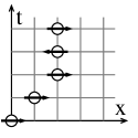
a) $\mathcal{H}_{\bot\mathnormal{1}}$

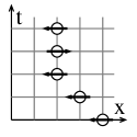
b) $\mathcal{H}_{\bot\mathnormal{2}}$

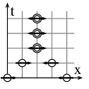
c) $\mathcal{H}_{\bot\mathnormal{1}}\odot\mathcal{H}_{\bot\mathnormal{2}}$

Fig. 12: “Pseudo-irreversible” process with QLGA

On the other hand, “a phase shift” due to interaction on Fig. 11 may be modelled using tensor product of two “slightly” nonequivalent qubots, but it is also possible with symmetric product of two qubots with extended internal space for counting time of “clinch”.

With infinite-dimensional internal space it is possible to make the time of “clinch” infinite, i.e., model process like non-elastic collision, usually considered as irreversible Fig. 12.

The Fock space for system with varying number of qubots may be introduced as

$$\mathcal{H}_{\top}=\mathop{\textstyle{\bigoplus}}\limits_{n=0}^{\infty}\mathcal{H}_{\top^{n}}.$$ (38)

2.3 QLGA and QCA

For antisymmetric product Eq. (38) has only finite number of terms. For lattice with $l$ nodes and $m$-dimensional internal space, there are $lm+1$ terms and $\dim\mathcal{H}_{\wedge}=2^{lm}$. So there is some difference with cellular automata with same lattice $l$ and internal space $\mathcal{H}_{S}$, because dimension of Hilbert space of such CA is $\dim\mathcal{H}_{L}=m^{l}$. Simplest identification is possible for a case $m=1$ for lattice gas and $m^{\prime}=2$ for cellular automaton ($\dim=2^{l}$)

$$\mathcal{H}_{\wedge}\cong\mathcal{H}_{L},\qquad\mathcal{H}_{\wedge}=\mathop{\textstyle{\bigoplus}}\limits_{n=0}^{l}\mathcal{H}_{\wedge^{n}},\quad\mathcal{H}_{L}=\mathop{\textstyle{\bigotimes}}\limits_{i=1}^{l}\mathcal{H}_{i}.$$ (39)

Similarly, an “antisymmetric” lattice gas with arbitrary $m$ may be formally represented either by cellular automaton with $m^{\prime}=2$, but with lattice extended by one new dimension $L^{\prime}=L\times m$, or CA with same lattice $L$ and $m^{\prime}=2^{m}$.

For symmetric case it is also possible to use similar transition from lattice gases to cellular automata. For example instead of lattice gas with $m=1$ and lattice $L$, it is possible to consider CA with same lattice, but $m=\infty$, here state of node in lattice is some $N\geq 0$, representing number of particles in given state.

Formally such transition from lattice gases to cellular automata in quantum case is equivalent to construction of “the Fock space for each cell”

$$\mathcal{H}_{F(S)}=\mathop{\textstyle{\bigoplus}}\limits_{n=0}^{\infty}\mathcal{H}_{S^{n}}$$ (40)

instead of Eq. (38) with Fock space for whole lattice and it may be disadvantage of such CA picture, if to recall global character of Fock space. It is especially clear, if to try to make some calculations in “discrete momentum space” related with initial lattice coordinates by discrete Fourier transform.

2.4 Space-Time Model of QLGA

For addition of the time dimension it is necessary instead of spatial lattice $\ell$ to consider space-time lattice $\ell^{\prime}=\ell\times{\mathbb{T}}$, i.e., to extend space $\mathcal{H}_{\ell}$ of each qubot, $\mathcal{H}_{\ell^{\prime}}=\mathcal{H}_{\ell}\otimes\mathcal{H}_{\mathbb{T}}$.

It is possible to write

$$\mathcal{H}_{\bot}=\mathcal{H}_{\ell}\otimes\mathcal{H}_{S}\cong\mathbb{C}^{n_{\ell}n_{S}},\quad\mathcal{H}_{\bot}^{\mathbb{T}}=\mathcal{H}_{\ell^{\prime}}\otimes\mathcal{H}_{S}\cong\mathbb{C}^{n_{\ell}n_{t}n_{S}},$$ (41)

where $n_{\ell}=\dim\mathcal{H}_{\ell}$ is number of points in initial lattice, e.g., $n_{\ell}=n_{x}n_{y}n_{z}$, $n_{t}$ is number of points (steps) in time dimension, and $n_{S}=\dim\mathcal{H}_{S}$ — dimension of internal space of qubot.

So for one-qubot state some analogue of Eq. (31) is really hold, because

$$n_{t}\to n_{t}+1\colon\quad\mathcal{H}_{\bot}^{\mathbb{T}}\to\mathcal{H}_{\bot}^{{\mathbb{T}}+1}\cong\mathcal{H}_{\bot}^{\mathbb{T}}\oplus\mathcal{H}_{\bot}.$$ (42)

On the other hand, let us consider Fock space with all possible antisymmetric products with different number of qubots

$$\mathcal{H}_{\wedge}^{\mathbb{T}}=\!\!\bigoplus_{k=0}^{n_{\ell}n_{t}n_{S}}\!\!\bigl{(}\mathop{\textstyle{\bigwedge}}\limits_{i=1}^{k}\mathcal{H}_{\bot}^{\mathbb{T}}\bigr{)},\quad\dim\mathcal{H}_{\wedge}^{\mathbb{T}}=2^{n_{\ell}n_{t}n_{S}}.$$ (43)

The space Eq. (43) may be formally identified with QCA with same space-time lattice $\ell^{\prime}$ and with number of states $2^{n_{S}}$ for each site of lattice. So here is held an analogue of Eq. (10), because simple calculation of dimension shows

$$n_{t}\to n_{t}+1\colon\quad\mathcal{H}_{\wedge}^{\mathbb{T}}\to\mathcal{H}_{\wedge}^{\mathbb{T}}\otimes\mathcal{H}_{\wedge}.$$ (44)

On the other hand, finding of direct equation for evolution of such a QCA starting with initial QLGA and Eq. (43) looks rather nontrivial.

2.5 Simplest Example of QLGA to QCA Conversion

Let us consider qubot with two states on lattice with one site and only two time steps. Let us use a simple scheme for notation depicted by presented diagram of four-dimensional Hilbert space $\mathcal{H}_{\bot}=\mathcal{H}_{\ell^{\prime}}\otimes\mathcal{H}_{S}$. Basic vectors of the one-qubot space are denoted as $|\,{}^{\circ}_{\bullet}\,{}^{\circ}_{\circ}\rangle,|\,{}^{\bullet}_{\circ}\,{}^{\circ}_{\circ}\rangle,|\,{}^{\circ}_{\circ}\,{}^{\circ}_{\bullet}\rangle,|\,{}^{\circ}_{\circ}\,{}^{\bullet}_{\circ}\rangle.$

For example state $(|\,{}^{\bullet}_{\circ}\,{}^{\circ}_{\circ}\rangle+|\,{}^{\circ}_{\circ}\,{}^{\circ}_{\bullet}\rangle)/\sqrt{2}$ corresponds to one qubot evolution with state $|{\uparrow}\rangle$ at $t=0$ and $|{\downarrow}\rangle$ at $t=1$. It is “additive” scheme Eq. (3). Two-steps evolution without change of state may be described as

$$\bigl{|}\psi_{\bot}\bigr{\rangle}=\alpha\,\bigl{(}|\,{}^{\circ}_{\bullet}\,{}^{\circ}_{\circ}\rangle+|\,{}^{\circ}_{\circ}\,{}^{\circ}_{\bullet}\rangle\bigr{)}+\beta\,\bigl{(}\bigl{|}\,{}^{\bullet}_{\circ}\,{}^{\circ}_{\circ}\bigr{\rangle}+\bigl{|}\,{}^{\circ}_{\circ}\,{}^{\bullet}_{\circ}\bigr{\rangle}\bigr{)}$$ (45)

The antisymmetric Fock space may be decomposed

$$\mathcal{H}_{\top}=\mathbb{C}\oplus\mathcal{H}_{\bot}\oplus\mathcal{H}_{\bot}{\wedge}\mathcal{H}_{\bot}\oplus\mathcal{H}_{\bot}{\wedge}\mathcal{H}_{\bot}{\wedge}\mathcal{H}_{\bot}\oplus\mathcal{H}_{\bot}{\wedge}\mathcal{H}_{\bot}{\wedge}\mathcal{H}_{\bot}{\wedge}\mathcal{H}_{\bot}.$$ (46)

To identify the space of QLGA with QCA, let us use the “spacetime” lattice with two sites for moments $t=0$ and $t=1$. In “multiplicative” scheme Eq. (1) Hilbert space $\mathcal{H}_{\bullet}$ of each site has four states

$$|\emptyset\rangle=|\,{}^{\circ}_{\circ}\rangle,\ |{\uparrow}\rangle=|\,{}^{\bullet}_{\circ}\rangle,\ |{\downarrow}\rangle=|\,{}^{\circ}_{\bullet}\rangle,\ |{\updownarrow}\rangle=|\,{}^{\bullet}_{\bullet}\rangle.$$ (47)

The states describe “Fock space of site”. Here “spatial” lattice has only one site and so $\mathcal{H}_{L}=\mathcal{H}_{\bullet}$. Now Hilbert space $\mathcal{H}_{\top}$ of Fock space Eq. (46) for system with varying number of qubots may be described as

$$\mathcal{H}_{\top}\cong\mathcal{H}_{L}^{\mathbb{T}}=\mathcal{H}_{L}\otimes\mathcal{H}_{L}.$$ (48)

Due to Eq. (48) each element of Eq. (46) may be described as tensor product of two states Eq. (47), e.g., $|\,{}^{\bullet}_{\circ}\,{}^{\circ}_{\circ}\rangle=|\,{}^{\bullet}_{\circ}\rangle|\,{}^{\circ}_{\circ}\rangle=|{\uparrow},\emptyset\rangle$, $|\,{}^{\bullet}_{\circ}\,{}^{\circ}_{\bullet}\rangle=|\,{}^{\bullet}_{\circ}\rangle|\,{}^{\circ}_{\bullet}\rangle=|{\uparrow},{\downarrow}\rangle$, etc.

So trivial QLGA evolution Eq. (45) may be rewritten for QCA as

$$|\psi_{\bot}\rangle=\alpha\,\bigl{(}|{\downarrow},\emptyset\rangle+|\emptyset,{\downarrow}\rangle\bigr{)}+\beta\,\bigl{(}|{\uparrow},\emptyset\rangle+\bigl{|}\emptyset,{\uparrow}\bigr{\rangle}\bigr{)}$$ (49)

On the other hand, basic vectors in each term $\Lambda^{k}_{4}\mathcal{H}_{\bot}$ of Eq. (46) may be depicted as

$$\mathbb{C}\cong\Lambda^{0}_{4}\mathcal{H}_{\bot} (\dim=1)~{}\colon \bigl{|}\,{}^{\circ}_{\circ}\,{}^{\circ}_{\circ}\bigr{\rangle}$$

$$\mathcal{H}_{\bot}\cong\Lambda^{1}_{4}\mathcal{H}_{\bot} (\dim=4)~{}\colon \bigl{|}\,{}^{\circ}_{\bullet}\,{}^{\circ}_{\circ}\bigr{\rangle},~{}\bigl{|}\,{}^{\bullet}_{\circ}\,{}^{\circ}_{\circ}\bigr{\rangle},~{}\bigl{|}\,{}^{\circ}_{\circ}\,{}^{\circ}_{\bullet}\bigr{\rangle},~{}\bigl{|}\,{}^{\circ}_{\circ}\,{}^{\bullet}_{\circ}\bigr{\rangle}$$

$$\Lambda^{2}_{4}\mathcal{H}_{\bot} (\dim=6)~{}\colon \bigl{|}\,{}^{\circ}_{\bullet}\,{}^{\circ}_{\bullet}\bigr{\rangle},~{}\bigl{|}\,{}^{\bullet}_{\circ}\,{}^{\bullet}_{\circ}\bigr{\rangle},~{}\bigl{|}\,{}^{\bullet}_{\circ}\,{}^{\circ}_{\bullet}\bigr{\rangle},~{}\bigl{|}\,{}^{\circ}_{\bullet}\,{}^{\bullet}_{\circ}\bigr{\rangle},~{}\bigl{|}\,{}^{\bullet}_{\bullet}\,{}^{\circ}_{\circ}\bigr{\rangle},~{}\bigl{|}\,{}^{\circ}_{\circ}\,{}^{\bullet}_{\bullet}\bigr{\rangle}$$

$$\mathcal{H}_{\bot}\cong\Lambda^{3}_{4}\mathcal{H}_{\bot} (\dim=4)~{}\colon \bigl{|}\,{}^{\bullet}_{\bullet}\,{}^{\bullet}_{\circ}\bigr{\rangle},~{}\bigl{|}\,{}^{\bullet}_{\bullet}\,{}^{\circ}_{\bullet}\bigr{\rangle},~{}\bigl{|}\,{}^{\bullet}_{\circ}\,{}^{\bullet}_{\bullet}\bigr{\rangle},~{}\bigl{|}\,{}^{\circ}_{\bullet}\,{}^{\bullet}_{\bullet}\bigr{\rangle}$$

$$\mathbb{C}\cong\Lambda^{4}_{4}\mathcal{H}_{\bot} (\dim=1)~{}\colon \bigl{|}\,{}^{\bullet}_{\bullet}\,{}^{\bullet}_{\bullet}\bigr{\rangle}$$

Antisymmetric (Grassmann) product of basic elements from $\Lambda^{k}_{4}\mathcal{H}_{\bot}$ may be calculated using associativity of the operation $\wedge$ and “union” rule

$$\begin{array}[]{|c||c|c|c|c|}\hline\cr\bigwedge&\phantom{-}\bigl{|}\,{}^{\circ}_{\bullet}\,{}^{\circ}_{\circ}\bigr{\rangle}&\phantom{-}\bigl{|}\,{}^{\bullet}_{\circ}\,{}^{\circ}_{\circ}\bigr{\rangle}&\phantom{-}\bigl{|}\,{}^{\circ}_{\circ}\,{}^{\circ}_{\bullet}\bigr{\rangle}&\phantom{-}\bigl{|}\,{}^{\circ}_{\circ}\,{}^{\bullet}_{\circ}\bigr{\rangle}\\ \hline\cr\hline\cr\bigl{|}\,{}^{\circ}_{\bullet}\,{}^{\circ}_{\circ}\bigr{\rangle}&0&\phantom{-}\bigl{|}\,{}^{\bullet}_{\bullet}\,{}^{\circ}_{\circ}\bigr{\rangle}&\phantom{-}\bigl{|}\,{}^{\circ}_{\bullet}\,{}^{\circ}_{\bullet}\bigr{\rangle}&\phantom{-}\bigl{|}\,{}^{\circ}_{\bullet}\,{}^{\bullet}_{\circ}\bigr{\rangle}\\ \hline\cr\bigl{|}\,{}^{\bullet}_{\circ}\,{}^{\circ}_{\circ}\bigr{\rangle}&-\bigl{|}\,{}^{\bullet}_{\bullet}\,{}^{\circ}_{\circ}\bigr{\rangle}&0&\phantom{-}\bigl{|}\,{}^{\bullet}_{\circ}\,{}^{\circ}_{\bullet}\bigr{\rangle}&\phantom{-}\bigl{|}\,{}^{\bullet}_{\circ}\,{}^{\bullet}_{\circ}\bigr{\rangle}\\ \hline\cr\bigl{|}\,{}^{\circ}_{\circ}\,{}^{\circ}_{\bullet}\bigr{\rangle}&-\bigl{|}\,{}^{\circ}_{\bullet}\,{}^{\circ}_{\bullet}\bigr{\rangle}&-\bigl{|}\,{}^{\bullet}_{\circ}\,{}^{\circ}_{\bullet}\bigr{\rangle}&0&\phantom{-}\bigl{|}\,{}^{\circ}_{\circ}\,{}^{\bullet}_{\bullet}\bigr{\rangle}\\ \hline\cr\bigl{|}\,{}^{\circ}_{\circ}\,{}^{\bullet}_{\circ}\bigr{\rangle}&-\bigl{|}\,{}^{\circ}_{\bullet}\,{}^{\bullet}_{\circ}\bigr{\rangle}&-\bigl{|}\,{}^{\bullet}_{\circ}\,{}^{\bullet}_{\circ}\bigr{\rangle}&-\bigl{|}\,{}^{\circ}_{\circ}\,{}^{\bullet}_{\bullet}\bigr{\rangle}&0\\ \hline\cr\end{array}\qquad$$ (50)

$$\begin{array}[]{|c||c|c|c|c|c|c|}\hline\cr\bigwedge&\phantom{-}\bigl{|}\,{}^{\bullet}_{\bullet}\,{}^{\circ}_{\circ}\bigr{\rangle}&\phantom{-}\bigl{|}\,{}^{\circ}_{\bullet}\,{}^{\circ}_{\bullet}\bigr{\rangle}&\phantom{-}\bigl{|}\,{}^{\circ}_{\bullet}\,{}^{\bullet}_{\circ}\bigr{\rangle}&\phantom{-}\bigl{|}\,{}^{\bullet}_{\circ}\,{}^{\circ}_{\bullet}\bigr{\rangle}&\phantom{-}\bigl{|}\,{}^{\bullet}_{\circ}\,{}^{\bullet}_{\circ}\bigr{\rangle}&\phantom{-}\bigl{|}\,{}^{\circ}_{\circ}\,{}^{\bullet}_{\bullet}\bigr{\rangle}\\ \hline\cr\hline\cr\bigl{|}\,{}^{\circ}_{\bullet}\,{}^{\circ}_{\circ}\bigr{\rangle}&0&0&0&\phantom{-}\bigl{|}\,{}^{\bullet}_{\bullet}\,{}^{\circ}_{\bullet}\bigr{\rangle}&\phantom{-}\bigl{|}\,{}^{\bullet}_{\bullet}\,{}^{\bullet}_{\circ}\bigr{\rangle}&\phantom{-}\bigl{|}\,{}^{\circ}_{\bullet}\,{}^{\bullet}_{\bullet}\bigr{\rangle}\\ \hline\cr\bigl{|}\,{}^{\bullet}_{\circ}\,{}^{\circ}_{\circ}\bigr{\rangle}&0&-\bigl{|}\,{}^{\bullet}_{\bullet}\,{}^{\circ}_{\bullet}\bigr{\rangle}&-\bigl{|}\,{}^{\bullet}_{\bullet}\,{}^{\bullet}_{\circ}\bigr{\rangle}&0&0&\phantom{-}\bigl{|}\,{}^{\bullet}_{\circ}\,{}^{\bullet}_{\bullet}\bigr{\rangle}\\ \hline\cr\bigl{|}\,{}^{\circ}_{\circ}\,{}^{\circ}_{\bullet}\bigr{\rangle}&\phantom{-}\bigl{|}\,{}^{\bullet}_{\bullet}\,{}^{\circ}_{\bullet}\bigr{\rangle}&0&-\bigl{|}\,{}^{\circ}_{\bullet}\,{}^{\bullet}_{\bullet}\bigr{\rangle}&0&-\bigl{|}\,{}^{\bullet}_{\circ}\,{}^{\bullet}_{\bullet}\bigr{\rangle}&0\\ \hline\cr\bigl{|}\,{}^{\circ}_{\circ}\,{}^{\bullet}_{\circ}\bigr{\rangle}&\phantom{-}\bigl{|}\,{}^{\bullet}_{\bullet}\,{}^{\bullet}_{\circ}\bigr{\rangle}&\phantom{-}\bigl{|}\,{}^{\circ}_{\bullet}\,{}^{\bullet}_{\bullet}\bigr{\rangle}&0&\phantom{-}\bigl{|}\,{}^{\bullet}_{\circ}\,{}^{\bullet}_{\bullet}\bigr{\rangle}&0&0\\ \hline\cr\end{array}$$ (50^′)

$$\bigl{|}\,{}^{\bullet}_{\bullet}\,{}^{\bullet}_{\bullet}\bigr{\rangle}=\bigl{|}\,{}^{\circ}_{\bullet}\,{}^{\circ}_{\circ}\bigr{\rangle}\mathop{\textstyle{\bigwedge}}\limits\bigl{|}\,{}^{\bullet}_{\circ}\,{}^{\bullet}_{\bullet}\bigr{\rangle}=-\bigl{|}\,{}^{\bullet}_{\circ}\,{}^{\circ}_{\circ}\bigr{\rangle}\mathop{\textstyle{\bigwedge}}\limits\bigl{|}\,{}^{\circ}_{\bullet}\,{}^{\bullet}_{\bullet}\bigr{\rangle}=\bigl{|}\,{}^{\circ}_{\circ}\,{}^{\circ}_{\bullet}\bigr{\rangle}\mathop{\textstyle{\bigwedge}}\limits\bigl{|}\,{}^{\bullet}_{\bullet}\,{}^{\bullet}_{\circ}\bigr{\rangle}=-\bigl{|}\,{}^{\circ}_{\circ}\,{}^{\bullet}_{\circ}\bigr{\rangle}\mathop{\textstyle{\bigwedge}}\limits\bigl{|}\,{}^{\bullet}_{\bullet}\,{}^{\circ}_{\bullet}\bigr{\rangle}$$ (50^′′)

Now it is possible to calculate trivial evolution of two qubots, each one is described by Eq. (45) with different pair of coefficients

$$|\psi_{\bot\mathnormal{1}}\rangle\wedge|\psi_{\bot\mathnormal{2}}\rangle=(\alpha_{1}\beta_{2}-\alpha_{2}\beta_{1})\,\bigl{(}\bigl{|}\,{}^{\bullet}_{\bullet}\,{}^{\circ}_{\circ}\bigr{\rangle}+\bigl{|}\,{}^{\circ}_{\circ}\,{}^{\bullet}_{\bullet}\bigr{\rangle}-\bigl{|}\,{}^{\bullet}_{\circ}\,{}^{\circ}_{\bullet}\bigr{\rangle}+\bigl{|}\,{}^{\circ}_{\bullet}\,{}^{\bullet}_{\circ}\bigr{\rangle}\bigr{)}.$$ (51)

So for equal states it is zero and for nonequal qubots after normalization it is always the same “Bell-like” state

$$\frac{1}{2}\bigl{(}\bigl{|}{\updownarrow},\emptyset\bigr{\rangle}+\bigl{|}\emptyset,{\updownarrow}\bigr{\rangle}+\bigl{|}{\downarrow},{\uparrow}\bigr{\rangle}-\bigl{|}{\uparrow},{\downarrow}\bigr{\rangle}\bigl{)}.$$ (52)

References

- [1] B. Schumacher and R. F. Werner, “Reversible quantum cellular automata,” quant-ph/0405174.
- [2] R. Cleve, A. K. Ekert, L. Henderson, C. Macchiavello, and M. Mosca, “On quantum algorithms”, Complexity 4, 33–42 (1998), quant-ph/9903061.
- [3] S. Wolfram, Cellular automata and complexity: Collected papers, (Addison-Wesley, Reading MA 1994).
- [4] T. Toffoli and N. Margolus, “Invertible cellular automata: a review,” Physica D 45, 229–253 (1990) .
- [5] C. H. Bennett, “Logical reversibility of computations,” IBM J. Res. & Dev. 17, 525–532 (1973).
- [6] P. Benioff, “Quantum mechanical Hamiltonian models of discrete processes that erase their own histories: Application to Turing machines,” Int. J. Theor. Phys. 21, 177–201 (1982).
- [7] M. Gardner, Wheels, Life and other mathematical amusements, (Freeman, San Francisco, 1983).
- [8] W. K. Wootters and W. H. Zurek, “A single quantum cannot be cloned,” Nature 299, 802–803 (1982).
- [9] D. A. Meyer, “From quantum cellular automata to quantum lattice gases,” J. Stat. Phys. 85, 551–574 (1996), quant-ph/9604003.
- [10] D. A. Meyer, “Quantum mechanics of lattice gas automata. I,” Phys. Rev. E 55, 5261–5269 (1997), quant-ph/9611005. D. A. Meyer, “Quantum mechanics of lattice gas automata. II,” J. Phys. A 31, 2321–2340 (1998), quant-ph/9712052.
- [11] A. Yu. Vlasov, “Quantum ‘bots’ on lattices,” unpublished, (ISI Foundation, Think-tank on “Computer Science Aspects,” Torino, Villa Gualino, Italy, 19–30 June 2000).
- [12] P. Benioff, “Quantum robots and environments,” Phys. Rev. A 58, 893–904 (1998), quant-ph/9802067
- [13] A. Barenco, D. Deutsch, A. K. Ekert, and R. Jozsa, “Conditional quantum dynamics and logic gates,” Phys. Rev. Lett. 74, 4083–4086 (1995).
- [14] D. Aharonov, A. Ambainis, J. Kempe, and U. Vazirani, “Quantum walks on graphs”, in Proc. 33th ACM STOC, 50–59 (2001), quant-ph/0012090.
- [15] A. M. Childs, R. Cleve, E. Deotto, E. Farhi, S. Gutmann, and D. A. Spielman, “Exponential algorithmic speedup by quantum walk,” in Proc. 35th ACM STOC, 59–68 (2003), quant-ph/0209131.