Quantum computing with magnetically interacting atoms

Abstract

We propose a scalable quantum-computing architecture based on cold atoms confined to sites of a tight optical lattice. The lattice is placed in a non-uniform magnetic field and the resulting Zeeman sublevels define qubit states. Microwave pulses tuned to space-dependent resonant frequencies are used for individual addressing. The atoms interact via magnetic-dipole interactions allowing implementation of a universal controlled-NOT gate. The resulting gate operation times for alkalis are on the order of milliseconds, much faster then the anticipated decoherence times. Single qubit operations take about 10 microseconds. Analysis of motional decoherence due to NOT operations is given. We also comment on the improved feasibility of the proposed architecture with complex open-shell atoms, such as Cr, Eu and metastable alkaline-earth atoms with larger magnetic moments.

I Introduction

Over the last decade, a variety of architectures for quantum computing (QC) has been proposed QCe . In particular there is a number of proposals based on neutral atoms and molecules trapped in optical lattices. These proposals focus on various realizations of the multi-qubit logic such as Rydberg-atom gates Jaksch et al. (2000), controlled collisions Jaksch et al. (1999); You and Chapman (2000); Brennen et al. (2002), electrostatic interaction of heteronuclear molecules DeMille (2002), etc (see a popular review Cirac and Zoller (March 2004).) While there is a variety of approaches available, the technological difficulties so far impede practical implementation of these schemes. Here we propose a scalable quantum-computing architecture which further builds upon the well-established techniques of atom trapping. Compared to the popular neutral-atom QC scheme with Rydberg gates Jaksch et al. (2000), the distinct features of the present proposal are: (i) individual addressing of atoms confined to sites of 1D optical lattice with unfocused beams of microwave radiation, (ii) coherent “always-on” magnetic-dipolar interactions between the atoms, and (iii) substantial decoupling of the motional and inner degrees of freedom. The Hamiltonian of our system is identical to that of the QC based on nuclear magnetic resonance (NMR) R. Laflamme et al. (2002), and already designed algorithms can be adopted for carrying computations with our quantum processor. An implementation of the celebrated Shor’s algorithm with a linear array of qubits has been discussed recentlyFowler et al. .

One of the challenges in choosing the physical system suitable for QC is the strength of the interparticle interaction. Before proceeding with the main discussion, let us elaborate on the suitability of magnetic-dipolar atom-atom interactions for QC. Compared to the dominant electrostatic interaction between a pair of atoms, magnetic-dipole interaction between a pair of atoms is weak (it is suppressed by a relativistic factor of $\alpha^{2}\approx(1/137)^{2}$.) Yet the dipolar interaction exhibits a pronounced anisotropic character: the strength and the sign of the interaction depend on a mutual orientation of magnetic moments of the two atoms. Namely the anisotropy of the interaction plays a decisive role in realizing a universal element of quantum logic: the two-qubit controlled-NOT (CNOT) gate Barenco et al. (1995). As to the strength of the interaction, it determines how fast the two-qubit gate operates. As the interaction strength decreases, the operation time, $\tau_{\mathrm{CNOT}}$, increases. Still, quantitatively, the operation of the gate must be much faster than decoherence. For atoms in far-off-resonance optical lattices, the decoherence times for internal (hyperfine) states, chosen as qubit states, are anticipated to be in the order of minutes qis . On the other hand, we show that for magnetically-interacting atoms placed in tight optical lattices $\tau_{\mathrm{CNOT}}$ is a few milli-second long. Thus, although the interaction is weak, it is still strong enough to allow for more than $10^{4}$ operations on a pair of qubits. Considering that trapping millions of atoms is common now, the scalable quantum computer (QC) proposed here may present a competitive alternative to other architectures.

According to DiVincenzo (2000), the physical implementation of QC should satisfy the following five criteria: (i) A scalable physical system with a well-characterized qubit; (ii) The ability to initialize the state of the qubit to a simple fiducial state; (iii) A “universal” set of quantum gates; (iv) Long relevant decoherence times, much longer than the gate operation time; (v) A qubit-specific measurement capability. Below, while describing our proposed QC, we explicitly address these criteria. We also compare it with QC based on nuclear magnetic resonance (NMR) techniques R. Laflamme et al. (2002), because of the equivalence of multiparticle Hamiltonians of our QC and the NMR systems. Unless noted otherwise, atomic units $|e|=m_{e}=\hbar\equiv 1$ are used throughout; in these units the Bohr magneton $\mu_{B}=1/2$.

II Choice of qubit

We focus on alkali-metal atoms in their respective ground ${}^{2}\!S_{1/2}$ state, but later (Section VI) also comment on the improved feasibility of our QC for other open-shell ground state and metastable atoms. The atoms are placed in a magnetic field and the resulting Zeeman components define qubit states. As shown in Fig. 1 for ²³Na, the Zeeman energies behave non-linearly as a function of the magnetic field strength $B$. The non-linearity is due to an interplay between couplings of atomic electrons to the nuclear and the externally-applied fields. The discussion presented below can be extended to an arbitrary field strength, but for illustration we consider the high-field limit, $\mu_{B}B\gg\Delta E_{\mathrm{HFS}}/(2I+1)$. Here $\Delta E_{\mathrm{HFS}}$ is the hyperfine splitting that ranges from 228 MHz for ⁶Li to 9193 MHz in ¹³³Cs and $I$ is the nuclear spin. In this regime, the proper lowest-order states are product states $|J,M_{J}\rangle|I,M_{I}\rangle$, where $M_{J}$ and $M_{I}$ are projections of the total electronic momentum $J=1/2$ and the nuclear spin $I$ along the B-field. We choose the qubit states as $|1\rangle\equiv|J,M_{J}=1/2\rangle|I,M_{I}\rangle$ and $|0\rangle\equiv|J,M_{J}=-1/2\rangle|I,M_{I}\rangle$. Disregarding nuclear moment, these states have magnetic moments of $\mu_{|1\rangle}=\mu_{B}$ and $\mu_{|0\rangle}=-\mu_{B}$, and the associated Zeeman splitting is on the order of a few GHz (see Fig.1). This choice allows driving single-qubit unitary operations with microwave (MW) pulses. The MW radiation has to be resonant with the Zeeman frequency $\left(\mu_{|1\rangle}-\mu_{|0\rangle}\right)B$.

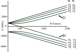
Figure 1: Zeeman effect for the ground state of ²³Na atom. The states are labeled with the electronic and nuclear magnetic quantum numbers $M_{J}$ and $M_{I}$ in the strong-field limit. A possible choice of qubit states is shown.

As to the initialization of the qubits of the proposed QC, the conventional techniques of optical pumping may be used. State-selective ionization may be employed for the read-out of the results of calculations. Ion optics for registering the final states is described in Ref. DeMille (2002). Both the initialization process and the projective readout favor the proposed QC in comparison to the liquid state NMR QC, where the ensemble averaging is required for read-out and relaxation of the sample is important for initialization.

III Individual addressability

In NMR R. Laflamme et al. (2002), the nuclear spins (qubits) are distinguished by their different chemical shifts affecting resonance spin-flip frequencies. Here to individually address the atoms, we confine ultracold atoms to sites of a one-dimensional optical lattice and introduce a gradient of magnetic field, so that the Zeeman frequency depends on the position of the atom in the lattice (see Fig.2). This addressing scheme was investigated in details in Ref. Mintert and Wunderlich (2001), in the context of quantum processor using trapped ions. It is also worth mentioning a similar idea for QC with heteronuclear diatomic molecules DeMille (2002), where a gradient of electric field was applied along optical lattice affecting flip frequencies of molecular dipoles.

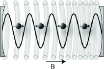
Figure 2: Proposed quantum computing architecture. The atoms are confined to sites of an optical lattice. Non-uniform magnetic field is required for individual addressing of the atoms with pulses of the resonant microwave radiation.

III.1 Optical lattice

The 1D potential of the optical lattice created by a standing wave CW laser beam reads $V_{\mathrm{opt}}(z)=V_{0}\sin^{2}\left(\frac{2\pi}{\lambda}z\right)$. The depth of the wells is $V_{0}=8\pi\alpha\times\alpha_{a}(\omega)I_{L}$, where $\alpha_{a}(\omega_{L})$ is the dynamic electric-dipole polarizability of the atom, $I_{L}$ is the laser intensity, and $\alpha\approx 1/137$ is the fine-structure constant. Depending on the detuning of the laser frequency $\omega_{L}$ from a position of atomic resonance, the polarizability can accept a wide range of values. To restrict the transverse atomic motion in a 1D optical lattice one must require that $\alpha_{a}(\omega_{L})>0$. The case of negative $\alpha_{a}(\omega_{L})$, although requiring 3D optical lattice, offers an advantage of reduced photon scattering rates. Since the atoms would be located at the intensity minima, the rates (in a tight confinement regime) would be suppressed by a factor of $1/2\sqrt{E_{R}/V_{0}}\ll 1$, where $E_{R}=\alpha^{2}\omega_{L}^{2}/(2M)$ is the photon recoil energy for an atom of mass $M$. Further, an atom is assumed to occupy the ground motional state of the lattice wells and one atom per site filling ratio is assumed. Techniques for loading optical lattices are being perfected lat ; Brennen et al. .

In the 1D optical lattice, the neighboring atoms are separated by a distance of $R=\lambda/2$. To maximize the magnetic-dipole interaction ($\propto 1/R^{3}$) between two neighbors we require that the frequency of the laser $\omega_{L}$ is chosen as high as possible. A natural limit on $\omega_{L}$ is the ionization potential (IP) which ranges from 3.8 eV for Cs to 5.4 eV for Li. Practically, $\omega_{L}$ must be somewhat below the IP to avoid resonances in the high-density of states near the continuum limit. In the estimates below we use $\omega_{L}\sim 5$ eV. This corresponds to

$$\lambda_{L}\approx 250\,\mathrm{nm}=4700\,\text{bohr}\,.$$

While working with such short ultra-violet wavelengths seems feasible, more conventional wavelenghts of $400-600\mathrm{nm}$ are adequate when working with complex open-shell atoms with larger magnetic moments (see Section VI).

One additional requirement is that the tunneling time between adjacent sites of an optical lattice is sufficiently long, so that the atoms maintain their distinguishability during the computation. The site-hoping frequency can be estimated as Brennen et al.

$$J=E_{R}\frac{4}{\sqrt{\pi}}\left(\frac{V_{0}}{E_{R}}\right)^{3/4}\exp\left[-2\sqrt{V_{0}/E_{R}}\right].$$

For ${}^{23}\mathrm{Na}$, the requirement that the characteristic tunneling time $\pi/J\approx 10\,\mathrm{sec}$ leads to a barrier hight of $V_{0}=0.4\,\mathrm{mK}$. At a fixed $\omega_{L}$, the tunneling may be suppressed by increasing the barrier height $V_{0}$ and by using heavier atoms. Additionally, due to the Pauli exclusion principle, the tunneling may be suppressed by using fermionic atoms.

III.2 B-field gradients

The magnetic field leads to the field-dependent Zeeman effect and the gradient $dB/dz$ of the B-field allows one to resolve the resonant frequencies of individual atoms, see Fig. 2. In the Section IV, we show that a typical two-qubit operation has a duration $\tau_{\mathrm{CNOT}}$ of a few milliseconds. To find the gradient $dB/dz$ we require that the single-qubit NOT operation, performed by the resonant $\pi$-pulse of microwave radiation, takes a comparable time $\tau_{\mathrm{NOT}}$ of 1 ms. Such pulse may be resolved by two neighboring atoms, provided that their resonant frequencies differ by $\Delta f_{\mathrm{NOT}}=1/(2\pi\tau_{\mathrm{NOT}})\approx 2\times 10^{2}\,\mathrm{Hz}$. The required field gradient is relatively weak

$$dB/dz\approx 20\,\mathrm{G/cm}$$

and is comparable to typical gradients in conventional magnetic traps. Much steeper gradients of $3\times 10^{3}\,\mathrm{G/cm}$ over a region of a few millimeters have been demonstrated by Vuletic et al. (1996). These authors employed ferromagnetic needles that collect and focus B-fields of electromagnetic coils. With such gradients the performance of the single- qubit gates can be substantially improved, $\tau_{\mathrm{NOT}}\sim 10\,\mu\mathrm{s}$.

Another limitation on the gradients is that the magnetic force $\mu dB/dz$ must be much smaller than the optical force $-dV_{\mathrm{opt}}(z)/dz$. This limitation affects not only the confinement but also a degree of coupling of inner and motional degrees of freedom because of the difference in values of magnetic moments for the two qubit states (see Section V.1). For the parameters chosen above the magnetic forces are several orders of magnitude smaller than the optical ones.

IV Multi-qubit operations

Having discussed one-qubit operations, we now consider a realization of the universal controlled-NOT gate Barenco et al. (1995) based on magnetic-dipolar interaction of two atoms. It is worth mentioning that we discuss this gate here only for illustrative purposes, to estimate the characteristic duration of the CNOT operation, $\tau_{\mathrm{CNOT}}$. The many-body dynamics of the system with the interparticle interaction which is “always on” is such that the two-qubit gates are executed as a part of the natural dynamics of the system, and a special care has to taken to govern this natural evolution Leung et al. (2000). We will elaborate on this point at the end of this Section.

The basic requirement for the controlled-NOT gate Barenco et al. (1995) is that the frequency of $|1\rangle\rightarrow|0\rangle$ transition of the target atom depends on the state of the control atom. Since the quantization (B-field) axis is directed along the internuclear separation between the two atoms, the magnetic-dipole interaction can be represented as

$$V=-\frac{\alpha^{2}}{R^{3}}\sum_{\lambda=-1}^{1}(1+\delta_{\lambda,0})\mu_{\lambda}(1)\mu_{-\lambda}(2)\,,$$ (1)

where $\mu_{\lambda}(k)$ represents the spherical components of the magnetic moment operator $\bm{\mu}$ for atom $k$. For performing the CNOT gate operation we need to resolve the frequency difference of $2\alpha^{2}R^{-3}\left(\mu_{|1\rangle}-\mu_{|0\rangle}\right)^{2}$. For our choice of parameters we find that $\Delta f_{\mathrm{CNOT}}\approx 40\,\mathrm{Hz}$. Although this number may seem small, it is comparable to typical coupling strengths of 20-200 Hz in NMR. Furthermore, the minimum duration of the MW pulse is $\tau_{\mathrm{CNOT}}=1/(2\pi\Delta f_{\mathrm{CNOT}})\approx 3\,\mathrm{ms}$, allowing for more than $10^{4}$ CNOT operations during anticipated decoherence time (in the order of minutes qis ).

As in the NMR, the interaction between the atoms is always on and special care has to be taken to stop the undesired time evolution of the system and carry out controlled calculations. Fortunately, it is straightforward to show that the many-particle Hamiltonian of our system is equivalent to that of a system of interacting spins in NMR and thus already developed techniques can be adopted. Specifically, the Hamiltonian is

$$H_{\mathrm{NMR}}=\sum_{i}\omega_{i}\left(\sigma_{z}\right)_{i}+\frac{1}{2}\sum_{ij}g_{ij}\left(\sigma_{z}\right)_{i}\left(\sigma_{z}\right)_{j}.$$ (2)

Here $\left(\sigma_{z}\right)_{i}$ are the Pauli matrices for an atom $i$ located at position $z_{i}$. Introducing the average magnetic moment $\bar{\mu}=(\mu_{|1\rangle}+\mu_{|0\rangle})/2$ and the difference $\delta\mu=(\mu_{|1\rangle}-\mu_{|0\rangle})/2$, the one-particle frequencies may be expressed as

$$\omega_{i}=-\delta\mu_{i}B\left(z_{i}\right)+\sum_{j}\frac{2\alpha^{2}}{|z_{i}-z_{j}|^{3}}\bar{\mu}_{j}\delta\mu_{i}$$

and the two-body couplings as

$$g_{ij}=-2\alpha^{2}/(|z_{i}-z_{j}|^{3})\,\delta\mu_{i}\delta\mu_{j}\,.$$

Since the Hamiltonian $H_{\mathrm{NMR}}$, Eq.(2), is identical to that of the NMR based QC Leung et al. (2000), the already developed NMR algorithms can be adopted. For example, the time evolution for a given atom may be reversed by inverting populations. The same idea is applicable for the interparticle couplings. The CNOT gate may be implemented by applying a sequence of one-qubit transformations (short pulses) and allowing a given coupling to develop in time Leung et al. (2000). An implementation of the celebrated Shor’s algorithm on the system of linear array of qubits has been discussed recently by Fowler et al. .

An important point is that the two-particle couplings result in a coherent development of the system. As we demonstrate below, the short NOT pulses introduce negligible decoherences due to excitation of motional quanta during the gate operation.

V Decoherences

Finally, we address possible sources of decoherences. We divide these sources into two classes: (i) induced due to the required operation of the quantum processor (due to performing gates) and (ii) architectural, i.e., due to traditional sources of decoherences, such as photon scattering (e.g. Raman), instabilities of laser output, instabilities in the magnetic field, collisions with background gas, etc. Below we analyze the decoherences caused by the gate operations and we also estimate the upper limit on tolerable fluctuations of the magnetic field. The remaining decoherences depend on the details of experimental design, e.g., laser wavelengths available, and we can not fully address them at this point.

V.1 Motional heating

The atomic center-of-mass (C.M.) evolves in a combined potential of the optical lattice and magnetic field. This potential depends on the internal state of the atom, due to a difference in dynamic polarizabilities and magnetic moments of the states. When population is transferred from one qubit (internal) state to the other, the motion of the C.M. is perturbed and the atom may leave the ground state of C.M. potential (motional heating). Here we calculate the relevant probability and show that it is negligible. We find that the motional heating is suppressed due to adiabaticity of the population-transfer process. In other words, the inner and motional degrees of freedom decouple because our quantum processor is relatively slow. It is worth emphasizing that in the popular neutral-atom QC proposal Jaksch et al. (2000), the operation of the gates is much faster and the motional heating is of concern Safronova et al. (2003).

As discussed in the previous section, the QC proposed here requires only single-qubit rotation pulses with a characteristic duration $\tau_{\mathrm{NOT}}$. The two-qubit gate operations are performed by the NOT pulses and due to the natural coherent dynamics of the system, so it sufficient to consider the coupling of the inner and motional degrees of freedom due to the NOT pulse only.

For a resonant radiation, during the MW pulse, the effective Hamiltonian may be represented as

$$H(\mathbf{R},\mathbf{r}) = \frac{\Omega}{2}\left(|0\rangle\langle 1|+|1\rangle\langle 0|\right)+$$

$$\frac{P^{2}}{2M}+V_{|1\rangle}\left(\mathbf{R}\right)|1\rangle\langle 1|+V_{|0\rangle}\left(\mathbf{R}\right)|0\rangle\langle 0|.$$

Here $\mathbf{R}$ and $\mathbf{P}$ are the C.M. coordinate and momentum, and $\mathbf{r}$ encapsulates internal degrees of freedom ($|0\rangle$ and $|1\rangle$). The internal states are coupled via $\Omega=\pi/\tau_{\mathrm{NOT}}$, the Rabi frequency of the MW transition. The C.M. evolves either in $V_{|0\rangle}$ or $V_{|1\rangle}$ potentials. We treat the difference between the C.M. potentials $W=V_{|1\rangle}-V_{|0\rangle}$ as a perturbation and characterize the C.M. motion with eigenstates $|\Phi_{n}\rangle$ and energies $\mathcal{E}_{n}$ computed in the $V_{|0\rangle}$ potential.

$$\left(\frac{P^{2}}{2M}+V_{|0\rangle}\left(\mathbf{R}\right)\right)|\Phi_{n}\rangle=\mathcal{E}_{n}|\Phi_{n}\rangle\,.$$

We assume that at $t=0$ the atom is in the motional and internal ground state $\Psi(\mathbf{R},\mathbf{r},t=0)=|0\rangle\,|\Phi_{0}\rangle$. As a result of the transfer of population (NOT operation, $|0\rangle\rightarrow|1\rangle$ ) there is a finite probability $P_{p}$ for an atom to end up in one of the excited motional eigenstates $|\Phi_{p}\rangle$.

We evaluate the probability $P_{p}$ perturbatively by expanding

$$\Psi(\mathbf{R},\mathbf{r},t)\approx a(t)|0\rangle\,|\Phi_{0}\rangle+b(t)|1\rangle\,|\Phi_{0}\rangle+c(t)|1\rangle\,|\Phi_{p}\rangle.$$

Substituting this expansion into the Schrodinger equation and solving it perturbatively (perturbation is $W$, the two-level Rabi evolution is treated exactly ) we obtain

$$a(t) \approx \sin(\Omega/2t)\,,$$

$$b(t) \approx \cos(\Omega/2t)\,,$$

$$i\frac{d}{dt}c\left(t\right) \approx \sin\left(\Omega/2t\right)\exp\left(i\omega_{p0}t\right)\langle\Phi_{p}|W|\Phi_{0}\rangle\,,$$

where $\omega_{p0}=\mathcal{E}_{p}-\mathcal{E}_{0}$. Calculation of the probability based on $c(t)$ requires certain care, since after the initial application of the pulse the perturbation $W$ remains on indefinitely. Using an approach discussed in Ref. Landau and Lifshitz (1997), we arrive at the probability of excitation

$$P_{p}(\tau_{\mathrm{NOT}})=\left|\frac{\langle\Phi_{p}|W|\Phi_{0}\rangle}{\omega_{p0}}\right|^{2}G\left(\frac{\Omega/2}{\omega_{p0}}\right),$$ (4)

where we introduced the adiabaticity function

$$G\left(\xi\right)=\frac{\xi^{2}}{\left(\xi^{2}-1\right)^{2}}\,\left(1+\xi^{2}-2\,\xi\,\sin(\frac{\pi}{2\,\xi})\right)\,.$$ (5)

This function is plotted in Fig. 3. The function is bounded $G\left(\xi\right)\leq 1$; there is no singularity at the resonant frequency $G(\xi=1)\approx 0.87$, since the C.M. experiences only a quarter of the period of oscillating function during the $\pi$ pulse. Let us investigate various limits of $G\left(\xi\right)$. For an instantaneous turn-on of the perturbation, $G(\xi\gg 1)\approx 1$, so that

$$P_{p}(\tau_{\mathrm{NOT}})=\left|\frac{\langle\Phi_{p}|W|\Phi_{0}\rangle}{\omega_{p0}}\right|^{2},\,\tau_{\mathrm{NOT}}\omega_{p0}\ll 1\,.$$

For a slow (adiabatic) application of the $\pi$-pulse $G(\xi\ll 1)\approx 1/\xi^{2}$. In this adiabatic limit

$$P_{p}(\tau_{\mathrm{NOT}})=\left|\frac{\langle\Phi_{p}|W|\Phi_{0}\rangle}{\Omega/2}\right|^{2}\,,\tau_{\mathrm{NOT}}\omega_{p0}\gg 1\,.$$

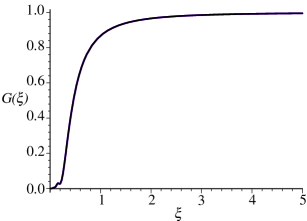
Figure 3: Adiabaticity function $G\left(\xi\right)$, Eq.(5).

Now we can carry out the numerical estimates. To compute the matrix elements of the perturbation, we approximate the bottom of the optical potential as that of harmonic oscillator of the frequency $\omega_{\mathrm{ho}}=\frac{2\pi}{\lambda_{L}}\sqrt{2V_{0}/M}$ and use the harmonic oscillator wavefunctions for $|\Phi_{n}\rangle$. For ²³Na and our lattice parameters ($\lambda_{L}\approx 250\,\mathrm{nm},V_{0}\approx 0.4\,\mathrm{mK}$ ), $\omega_{\mathrm{ho}}\approx 2\pi~{}\times~{}2\times 10^{6}\,\mathrm{Hz}$, while the Rabi frequency (for the extreme case of $dB/dz=2\times 10^{3}\mathrm{G/cm}$) $\Omega/2=2\pi\times 0.25\times 10^{5}\,\mathrm{Hz}$, i.e. even in the case of steep gradients we deal with an adiabatically slow pulse and the motional heating is suppressed by a factor of $\approx[\omega_{p0}/(\Omega/2)]^{2}$.

For a perturbation due to an interaction of magnetic moments with the gradient of magnetic field $W=\left(\mu_{|0\rangle}-\mu_{|1\rangle}\right)(dB/dz)z$. For our parameters, the probability of exciting motional quantum is just $P_{1}\sim 6\times 10^{-7}$.

Another source of coupling of internal and motional degrees of freedom is due to the difference in the dynamic polarizability $\alpha_{a}(\omega)$ for the two qubit states. This difference leads to a modification of $\omega_{\mathrm{ho}}\propto\sqrt{\alpha_{a}(\omega)}$. The relevant probability may be estimated as $P_{2}\approx G\left(\Omega/4\omega_{\mathrm{ho}}\right)\frac{1}{32}\left(2\mu_{B}B/\Delta\omega\right)^{2}\approx 10^{-10}\left(2\mu_{B}B/\Delta\omega\right)^{2}$, where $\Delta\omega$ is a detuning of the laser frequency from the energy of the intermediate state contributing the most to the dynamic polarizability $\alpha_{a}(\omega_{L})$. (Here we used the field gradient $dB/dz=20\mathrm{G/cm}$, so that $\tau_{\mathrm{NOT}}\approx\tau_{\mathrm{CNOT}}$, see section III.2.) In practice, $2\mu_{B}B/\Delta\omega\ll 1$, so that $P_{2}\ll 10^{-10}$. This probability can be reduced even further by adjusting the laser wavelength so that the dynamic polarizabilities of the two qubit states are the same Safronova et al. (2003).

Finally, we would like to emphasize that the motional heating is not an issue for our processor, because our QC is relatively slow. The C.M. cycles through many oscillations while the perturbing MW field is applied. This adiabatic averaging leads to the suppression of the motional heating.

V.2 Decoherences due to fluctuations of the magnetic field

The atoms in our quantum processor are required to have magnetic moments. This magnetic moments can couple to the ambient magnetic field. The fluctuations of these ambient fields can cause the qubit states to lose coherence. In addition, the Johnson/shot noise in the coils providing the gradient of the B-field can lead to the decoherences as well. Here we estimate the upper limit of tolerance to these fluctuations.

Before we carry out the estimate, we notice that the sensitivity to fluctuations of the magnetic fields can be avoided altogether using so-called Decoherence Free Subspaces (DFS) Duan and Guo (1998); Lidar et al. (1998); Zanardi and Rasetti (1997). The idea of the DFS is to redefine the qubit states using linear combinations of product of states of original qubits; each resulting state accumulates the same phase due to environmental interactions. Since the total phase of wavefunction is irrelevant, the DFS is highly stable with the respect to the external perturbations. This powerful DFS approach has been already experimentally verified in a number of cases, including trapped ions Kielpinski et al. (2001). Nevertheless, an introduction of the DFS requires reconsideration of the NMR algorithms, which is beyond the scope of the present paper. Below we estimate the decoherence of our original qubit defined as a couple of magnetic substates of an atom.

To make an order-of-magnitude estimate, we assume that the fluctuating field $B^{\prime}(t)$ is along the quantization axis and it has a white noise spectrum. With the fluctuating field present, the accumulated phase difference between the qubit states is $\delta\phi\approx 2\int_{0}^{t}\mu_{|0\rangle}B^{\prime}\left(t_{1}\right)dt_{1}$. (Here we assumed that $\mu_{|1\rangle}\approx-\mu_{|0\rangle}$.) Averaging over different realizations

$$\left\langle\exp\left(i\delta\phi\right)\right\rangle \approx 1+i\left\langle\delta\phi\right\rangle-\frac{1}{2}\left\langle\delta\phi^{2}\right\rangle$$

$$= 1+2i\int_{0}^{t}\mu_{|0\rangle}\left\langle B^{\prime}\left(t_{1}\right)\right\rangle dt_{1}$$

$$-2\mu_{|0\rangle}^{2}\int_{0}^{t}\int_{0}^{t}\left\langle B^{\prime}\left(t_{1}\right)B^{\prime}\left(t_{2}\right)\right\rangle dt_{1}dt_{2}\,.$$

This expression may be simplified using ensemble average $\left\langle B^{\prime}\left(t_{1}\right)\right\rangle=0$, and the autocorrelation function for a stochastic process with no memory

$$\left\langle B^{\prime}\left(t_{1}\right)B^{\prime}\left(t_{2}\right)\right\rangle=\left(B^{2}\right)_{\omega}\delta\left(t_{1}-t_{2}\right)\,,$$

where $\left(B^{2}\right)_{\omega}=\mathrm{const}$. If a measurement is carried out after $\tau_{\mathrm{CNOT}}$, the probabilities would differ from the exact result by

$$\varepsilon_{B}=(\left\langle\exp\left(i\delta\phi\right)\right\rangle-1)^{2}\approx 4\mu_{|0\rangle}^{2}~{}\left(B^{2}\right)_{\omega}\tau_{\mathrm{CNOT}}\,.$$

According to Knill , this error can be as high as 1%. This leads to a tolerable level of the B-field noise

$$\sqrt{\left(B^{2}\right)_{\omega}}\lesssim 10^{-10}\frac{\mathrm{T}}{\sqrt{\mathrm{Hz}}}\,.$$

This limit is relatively easy to attain experimentally Rom .

To summarize the main results of this section, we have demonstrated that for our quantum processor the motional heating caused by the gate operations is negligible. The derived formula  (4) is also applicable for an analysis of coupling of inner and motional degrees of freedom of QC based on heteronuclear molecules DeMille (2002). We also have evaluated the tolerable level of fluctuations in magnetic field. It is worth emphasizing that the sensitivity to environmental field noise can be greatly eliminated using decoherence free subspaces, as discussed in the beginning of this subsection.

There are other potential sources of decoherences, e.g. photon scattering, instabilities of laser output, and collisions with background gas. However, we do not address them at this point since they depend on specifics of experimental design. Still it is anticipated qis that the decoherence times for internal states may be in the order of minutes.

VI Complex open-shell atoms

In this paper we focused on alkali-metal atoms ($\mu=\mu_{B}$) and we found that wavelengths of $\lambda\sim 250$ nm are needed for $\tau_{\mathrm{CNOT}}\approx 3\,\mathrm{ms}$. While working with such short ultra-violet wavelengths still seems feasible, the restriction may be relaxed by using complex open-shell atoms with larger values of magnetic moments. This allows increasing the interaction strength ($\propto\mu^{2}$) and thus working with more conventional laser wavelengths.

For example, recently cooled and trapped Cr and Eu atomsCrE have magnetic moments of stretched states $\mu_{\mathrm{Cr}}=6\mu_{B}$ and $\mu_{\mathrm{Eu}}=7\mu_{B}$. Thus if a laser of a 400 nm wavelength is employed for constructing the optical lattice, the CNOT-gate operations would require $\tau_{\mathrm{CNOT}}\sim 0.1\,\mathrm{ms}$. The use of 30-mW violet 400 nm LD laser has been recently demonstrated in cooling and trapping experiments Park and Yoon (2003). The requirement $\tau_{\mathrm{CNOT}}\sim 1\,\mathrm{ms}$ would bring the wavelength to an even more practical 800 nm.

Another alternative is to use long-lived Derevianko (2001) metastable divalent atoms, Mg, Ca, Sr and Yb. Several groups have demonstrated cooling and trapping these atoms met , with Yb BEC recently attainedTakasu et al. (2003). Here the state of interest is ${}^{3}\!P_{2}$, with $\mu_{{}^{3}\!P_{2}}=3\mu_{B}$ and for a 400 nm laser $\tau_{\mathrm{CNOT}}\sim 1\,\mathrm{ms}$.

VII Conclusion

In summary, we proposed a scalable quantum computing architecture based on magnetically-interacting cold atoms confined to sites of a tight optical lattice. The atoms are placed in a non-uniform magnetic field and the individual addressing is attained by pulses of microwave radiation for a minimum duration of 10 $\mu$s. The universal two-qubit CNOT gates require times in the order of milliseconds. The multi-particle Hamiltonian of the system is equivalent to that of the QC based on NMR techniques so the already developed quantum algorithms may be adopted.

Compared to the popular neutral-atom QC scheme Jaksch et al. (2000), the distinct advantages of the present proposal are: (i) individual addressability of atoms with unfocused beams of microwave radiation, and (ii) coherent evolution due to the “always-on” magnetic-dipolar interactions between the atoms, (iii) substantial decoupling of the motional and inner degrees of freedom. While the main disadvantage of our QC is the slow rate of operation, it is anticipated that one could carry out $10^{4}$ CNOT operations on a single pair of atoms before the coherence is lost. When addressing tens of thousands of atoms is done in parallel, this would amass $10^{8}$ two-qubit operations and $10^{10}$ single-qubit operations.

- (1) Fortschr. Phys. 48, (2000), special focus issue on experimental proposals for quantum computation, edited by S. Braunstein and H.-K. Lo, and references therein.
- Jaksch et al. (2000) D. Jaksch, J. I. Cirac, P. Zoller, S. L. Rolston, R. Cote, and M. D. Lukin, Phys. Rev. Lett. 85, 2208 (2000).
- Jaksch et al. (1999) D. Jaksch, H.-J. Briegel, J. I. Cirac, C. W. Gardiner, and P. Zoller, Phys. Rev. Lett. 82, 1975 (1999).
- You and Chapman (2000) L. You and M. S. Chapman, Phys. Rev. A 62, 052302/1 (2000).
- Brennen et al. (2002) G. K. Brennen, I. H. Deutsch, and C. J. Williams, Phys. Rev. A 65, 022313/1 (2002).
- DeMille (2002) D. DeMille, Phys. Rev. Lett. 88, 067901 (2002).
- Cirac and Zoller (March 2004) J. I. Cirac and P. Zoller, Phys. Today pp. 38–44 (March 2004).
- R. Laflamme et al. (2002) R. Laflamme et al., Introduction to NMR quantum information processing (2002), arXiv:quant-ph/0207172.
- (9) A. G. Fowler, S. J. Devitt, and L. C. L. Hollenberg, quant-ph/0402196.
- Barenco et al. (1995) A. Barenco, D. Deutsch, A. Ekert, and R. Jozsa, Phys. Rev. Lett. 74, 4083 (1995).
- (11) Quantum Information Science and Technology Roadmap, Section 6.3: Neutral Atom Approaches to Quantum Information Processing and Quantum Computing, available from http://qist.lanl.gov.
- DiVincenzo (2000) D. DiVincenzo, Fortschr. Phys. 48, 771 (2000).
- Mintert and Wunderlich (2001) F. Mintert and C. Wunderlich, Phys. Rev. Lett. 87, 257904 (2001).
- (14) M. Greiner et al., Nature 415, 39 (2002); P. Rabl et al., Phys. Rev. Lett. 91, 110403 (2003).
- (15) G. K. Brennen, G. Pupillo, A. M. Rey, C. W. Clark, and C. J. Williams, e-print:quant-ph/0312069.
- Vuletic et al. (1996) V. Vuletic, T. W. Hänsch, and C. Zimmermann, Europhys. Lett. 36, 349 (1996).
- Leung et al. (2000) D. W. Leung, I. L. Chuang, F. Yamaguchi, and Y. Yamamoto, Phys. Rev. A 61, 042310/1 (2000).
- Safronova et al. (2003) M. S. Safronova, C. J. Williams, and C. W. Clark, Phys. Rev. A 67, 040303 (2003).
- Landau and Lifshitz (1997) L. D. Landau and E. M. Lifshitz, Quantum Mechanics, vol. III (Butterworth-Heinemann, 1997), 3rd ed.
- Duan and Guo (1998) L.-M. Duan and G.-C. Guo, Phys. Rev. A 57, 737 (1998).
- Lidar et al. (1998) D. Lidar, I. Chuang, and K. Whaley, Phys. Rev. Lett. 81, 2594 (1998).
- Zanardi and Rasetti (1997) P. Zanardi and M. Rasetti, Phys. Rev. Lett. 79, 3306 (1997).
- Kielpinski et al. (2001) D. Kielpinski, V. Meyer, M. Rowe, C. Sackett, W. Itano, C. Monroe, and D. Wineland, Science 291, 1013 (2001).
- (24) E. Knill, quant-ph/0404104.
- (25) M. Romalis, private communications.
- (26) J. Kim et al., Phys. Rev. Lett. 78, 3665 (1997); P. O. Schmidt et al., Phys. Rev. Lett. 91, 193201 (2003).
- Park and Yoon (2003) C. Y. Park and T. H. Yoon, Phys. Rev. A 68, 055401 (2003).
- Derevianko (2001) A. Derevianko, Phys. Rev. Lett. 87, 023002 (2001).
- (29) H. Katori et al., in Atomic Physics 17, edited by E. Arimondo, P. DeNatale, and M. Inguscia (AIP, New York, 2001); J. Grünert and A. Hemmerich, Phys. Rev. A 65, 041401 (2002); S. B. Nagel et al., Phys. Rev. A 67, 011401(R)(2003); X. Xu et al., J. Opt. Soc. Am. B 20, 968 (2003).
- Takasu et al. (2003) Y. Takasu, K. Maki, K. Komori, T. Takano, K. Honda, M. Kumakura, T. Yabuzaki, and Y. Takahashi, Phys. Rev. Lett. 91, 040404 (2003).