Conclusive and arbitrarily perfect quantum state transfer using parallel spin chain channels

Abstract

We suggest a protocol for perfect quantum communication through spin chain channels. By combining a dual-rail encoding with measurements only at the receiving end, we can get conclusively perfect state transfer, whose probability of success can be made arbitrarily close to unity. As an example of such an amplitude delaying channel, we show how two parallel Heisenberg spin chains can be used as quantum wires. Perfect state transfer with a probability of failure lower than $P$ in a Heisenberg chain of $N$ spin-$1/2$ particles can be achieved in a timescale of the order of $\frac{0.33\hbar}{J}N^{1.7}|\ln P|$. We demonstrate that our scheme is more robust to decoherence and non-optimal timing than any scheme using single spin chains.

I Introduction

The development of reliable methods to transfer quantum states is of fundamental importance in quantum information theory. Usually, flying qubits such as photons, ballistic electrons and guided atoms/ions are considered for this purpose. However, converting back and forth between stationary qubits (of say a quantum computer or as held by the communicating parties) and mobile carriers of quantum information and interfacing between different physical implementations of qubits is very difficult and may not be really worth for short communication distances.

An attractive alternative is to use a finite array of interacting but stationary qubits as an information bus. It would, however, not be very useful if the interactions between various pairs of stationary qubits have to be repeatedly switched on and off to perform the communication, because gating errors will then accumulate. Moreover, the local control required will be as high as that of a quantum computer. Only if we can utilize systems with permanently coupled material qubits (such as molecular spin chains), or systems without local control (such as Josephson junction arrays or optical lattices) with minimal global switchings, can we have a communication bus much before a quantum computer. In such schemes, both the amplitude and the phase damping (mechanisms of decoherence) can be ensured to be no worse than that of a single moving qubit, by ensuring that there is at most one excitation in the array during the communication process. With the above view in mind, recently the use of spin chains SB03 ; key-1 ; MCND+04 ; key-2 ; TJO04 ; key-3 ; FVMAM04 ; key-4 ; key-5 ; MYDL04 ; key-6 ; key-7 and harmonic chains PLENIO04 as quantum wires have been proposed.

The initial system independent proposal SB03 was inspired by the natural setting for spin chain molecules (and optical lattices): regular arrays without local accessibility. Single spin encoding was assumed to avoid quantum gates. For this simplicity, its specific realizations is already being proposed JOSEPH . However, it allows only imperfect communication fidelity and necessitate the use of entanglement distillation from a large ensemble, which destroy its simplicity. Later approaches of perfecting fidelity require either the engineering of the couplings MCND+04 ; key-2 , or an encoding of a qubit to several spins TJO04 ; key-3 . Independently, local measurements on each qubit along the chain FVMAM04 ; key-4 ; key-5 have been proposed. The above deviate either from naturalness or from simplicity. We are thus sorely in need of a scheme which remains natural and simple, yet achieves perfect quantum communication. This is achieved in this paper by using a dual-rail encoding.

The outline of the article is as follows. In Section II, we suggest a scheme for quantum communication using two parallel spin chains of the most natural type (namely those with constant couplings). We require modest encodings (or gates) and measurements only at the ends of the chains. The state transfer is conclusive, which means that it is possible to tell by the outcome of a quantum measurement, without destroying the state, if the transfer took place or not. If it did, then the transfer was perfect. The transmission time for conclusive transfer is no longer than for single spin chains. In Section III, we demonstrate that our scheme offers even more: if the transfer was not successful, then we can wait for some time and just repeat the measurement, without having to resend the state. By performing sufficiently many measurements, the probability for perfect transfer approaches unity. Hence the transfer is arbitrarily perfect. We will show in Section IV that the time needed to transfer a state with a given probability scales in a reasonable way with the length of the chain. Finally, in Section V we show that encoding to parallel chains and the conclusiveness also makes our protocol more robust to decoherence (a hitherto unaddressed issue in the field of quantum communication through spin chains).

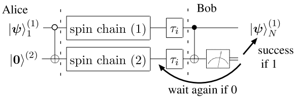
Figure 1: Quantum circuit representation of conclusive and arbitrarily perfect state transfer. The first gate at Alice’s qubits represents a NOT gate applied to the second qubit controlled by the first qubit being zero. The qubits $\left|\bm{\psi}\right\rangle_{1}^{(1)}$ on the left hand side represents an arbitrary input state at Alice’s site, and the qubit $\left|\bm{\psi}\right\rangle_{N}^{(1)}$ represents the same state, successfully transferred to Bob’s site. The $\tau_{i}$-gate represents the unitary evolution of the spin chains for a time interval of $\tau_{i}$.

II Scheme for conclusive transfer

We intend to propose our scheme in a system independent way with occasional references to systems where conditions required by our scheme are achieved. We assume that our system consists of two identical uncoupled spin-$1/2$-chains $(1)$ and $(2)$ of length $N$, described by the Hamiltonian

$$H=H^{(1)}\otimes I^{(2)}+I^{(1)}\otimes H^{(2)}-E_{g}I^{(1)}\otimes I^{(2)}.$$ (1)

The term identical states that $H^{(1)}$ and $H^{(2)}$ are the same apart from the label of the Hilbert space they act on. The requirement of parallel chains instead of just one is not problematic, since in many experimental realizations of spin chains, it is much easier to produce a whole bunch of parallel uncoupled NMEE96 ; GAMBARDELLA chains than just a single one.

We assume that the ground state of each chain is $\left|\mathbf{0}\right\rangle^{(i)}\equiv\left|0_{1}\ldots 0_{N}\right\rangle^{(i)}$, i.e. a ferromagnetic ground state, with $H^{(i)}\left|\mathbf{0}\right\rangle^{(i)}=E_{g}\left|\mathbf{0}\right\rangle^{(i)},$ and that the subspace consisting of the single spin excitations $\left|\mathbf{n}\right\rangle^{(i)}\equiv\sigma_{n}^{+(i)}\left|\mathbf{0}\right\rangle^{(i)}\,(n=1,\ldots,N)$ is invariant under $H^{(i)}.$ An arbitrary qubit at the site $n$ of system $(i)$ can be written as

$$\left|\bm{\psi}\right\rangle_{n}^{(i)}\equiv\alpha\left|\mathbf{0}\right\rangle^{(i)}+\beta\left|\mathbf{n}\right\rangle^{(i)}.$$ (2)

The dynamics restricted to this subspace can be expressed in terms of the transition amplitudes

$$f_{r,s}(t)\equiv\left\langle\mathbf{r}\right|^{(i)}e^{iH^{(i)}t}\left|\mathbf{s}\right\rangle^{(i)}.$$ (3)

The aim of our protocol is to transfer quantum information from the $1$st (“Alice”) to the $N$th (“Bob”) qubit of the first chain,

$$\left|\bm{\psi}\right\rangle_{1}^{(1)}\longrightarrow\left|\bm{\psi}\right\rangle_{N}^{(1)}.$$ (4)

To achieve this, we need $f_{1,N}(t)\neq 0$ (which is valid for a Heisenberg chain, for example SB03 ). An advantage of Heisenberg ferromagnetic chains over a non-interacting qubit array is that some XXZ anisotropy can make the states $\left|\mathbf{0}\right\rangle$ and $\left|\mathbf{n}\right\rangle$ stable against excitations at finite temperatures key-8 . Even a small anisotropy in the coupling $J$ may suffice (as $J$ itself can be as high as $2000K$ NMEE96 ). Alternatively, one can prevent thermal excitations by applying an uniform magnetic field to the chain.

The initial state of the system is $\left|\bm{\psi}\right\rangle_{1}^{(1)}\otimes\left|\mathbf{0}\right\rangle^{(2)}$. The first step of the protocol is to encode the input qubit in a “dual-rail” ILC96 by applying a NOT gate on the first qubit of system $(2)$ controlled by the first qubit of system $(1)$ being zero, resulting in a superposition of excitations in both systems,

$$\left|\mathbf{\bm{s}}(0)\right\rangle=\alpha\left|\mathbf{0}\right\rangle^{(1)}\otimes\left|\mathbf{1}\right\rangle^{(2)}+\beta\left|\mathbf{1}\right\rangle^{(1)}\otimes\left|\mathbf{0}\right\rangle^{(2)}.$$ (5)

This is assumed to take place in a much shorter timescale than the system dynamics. Even though a 2-qubit gate in solid state systems is difficult, such a gate for charge qubits has been reported TYYAP+03 . For the same qubits, Josephson arrays have been proposed as single spin chains for quantum communication JOSEPH . For this system, both requisites of our scheme are thus available. In fact, the demand that Alice and Bob can do measurements and apply gates to their local qubits (i.e. the ends of the chains) will be naturally fulfilled in practice since we are suggesting a scheme to transfer information between quantum computers.

Under the system Hamiltonian, the excitation in Eq. (5) will travel along the two systems. The state after the time $\tau_{1}$ can be written as

$$\left|\mathbf{\bm{\phi}}(\tau_{1})\right\rangle=\sum_{n=1}^{N}f_{n,1}(\tau_{1})\left|\mathbf{s}(n)\right\rangle,$$ (6)

where $\left|\mathbf{s}(n)\right\rangle=\alpha\left|\mathbf{0}\right\rangle^{(1)}\otimes\left|\mathbf{n}\right\rangle^{(2)}+\beta\left|\mathbf{n}\right\rangle^{(1)}\otimes\left|\mathbf{0}\right\rangle^{(2)}$. We can decode the qubit by applying a CNOT gate at Bob’s site. The state thereafter will be

$$\sum_{n=1}^{N-1}f_{n,1}(\tau_{1})\left|\mathbf{s}(n)\right\rangle+f{}_{N,1}(\tau_{1})\left|\bm{\psi}\right\rangle_{N}^{(1)}\otimes\left|\mathbf{N}\right\rangle^{(2)}.$$ (7)

Bob can now perform a measurement on his qubit of system $(2).$ If the outcome of this measurement is $1$, he can conclude that the state $\left|\bm{\psi}\right\rangle_{1}^{(1)}$ has been successfully transferred to him. This happens with the probability $\left|f_{N,1}(\tau_{1})\right|^{2}.$ If the outcome is $0$, the system is in the state

$$\frac{1}{\sqrt{P(1)}}\sum_{n=1}^{N-1}f_{n,1}(\tau_{1})\left|\mathbf{s}(n)\right\rangle,$$ (8)

where

$$P(1)=1-\left|f_{N,1}(\tau_{1})\right|^{2}$$ (9)

is the probability of failure for the first measurement. If the protocol stopped here, and Bob would just assume his state as the transferred one, the channel could be described as an amplitude damping channel, with exactly the same fidelity as the single chain scheme discussed in SB03 . But success probability is more valuable than fidelity: Bob has gained knowledge about his state, and may reject it and ask Alice to retransmit. However, as we will show in the next section, this is not necessary.

III Arbitrarily perfect state transfer

Because Bob’s measurement has not revealed anything about the input state, the information is still residing in the chain. By letting the state (8) evolve for another time $\tau_{2}$ and applying the CNOT gate again, Bob has another chance of receiving the input state. The state before performing the second measurement is easily seen to be

$$\frac{1}{\sqrt{P(1)}}\sum_{n=1}^{N}\left\{f_{n,1}(\tau_{2}+\tau_{1})-f_{n,N}(\tau_{2})f_{N,1}(\tau_{1})\right\}\left|\mathbf{s}(n)\right\rangle.$$ (10)

Hence the probability to receive the qubit at Bobs site at the second measurement is

$$\frac{1}{P(1)}\left|f_{N,1}(\tau_{2}+\tau_{1})-f_{N,N}(\tau_{2})f_{N,1}(\tau_{1})\right|^{2}.$$ (11)

If the transfer was still unsuccessful, this strategy can be repeated over and over. Each time Bob has a probability of failed state transfer that can be obtained from the generalization of Eq. (10) to an arbitrary number of iterations. The joint probability that Bob fails to receive the state all the time is just the product of these probabilities. We denote the joint probability of failure for having done $l$ unsuccessful measurements as $P(l)$. This probability depends on the time intervals $\tau_{i}$ between the $(i-1)$th and $i$th measurement, and we are interested in the case where the $\tau_{i}$ are chosen such that the transfer is fast. It is possible to write a simple algorithm that computes $P(l)$ for any transition amplitude $f_{r,s}(t).$ Figure 2 shows some results for a Heisenberg spin-$1/2$-chain with equal nearest neighbor couplings,

$$H^{(i)}=-J\sum\vec{\sigma}_{n}^{(i)}\cdot\vec{\sigma}_{n+1}^{(i)}.$$ (12)

This model is exactly solvable, and the transition amplitude is given explicitly in SB03 . However, the results are valid for a wide class of anisotropies and in the presence of a uniform magnetic field, too.

Figure 2: Semilogarithmic plot of the joint probability of failure $P(l)$ as a function of the number of measurements $l$. Shown are Heisenberg spin-$1/2$-chains with different lengths $N$. The times between measurements $\tau_{i}$ have been optimized numerically.

An interesting question is whether the joint probability of failure can be made arbitrary small with a large number of measurements. Since $P(l)$ is a bounded, monotonic decreasing series, it must have a limit. In fact, the times $\tau_{i}$ can be chosen such that the transfer becomes arbitrarily perfect. This has been proven in BBG , where a generalization of the above scheme and a much wider class of Hamiltonians is considered. In the limit of large number of measurements, the spin channel will not damp the initial amplitude, but only delay it.

IV Estimation of the timescale the transfer

The achievable fidelity is an important, but not the only criteria of a state transfer protocol. In this Section, we give an heuristic approach to estimate the time that it needs to achieve a certain fidelity in a Heisenberg spin chain. The comparison with numeric examples is confirming this approach.

Let us first describe the dynamic of the chain in a very qualitative way. Once Alice has initialized the system, an excitation wave packet will travel along the chain. As shown in SB03 , it will reach Bob at a time of the order of

$$\tau_{max}\approx\frac{\hbar N}{2J},$$ (13)

with an amplitude of

$$\left|f_{N,1}(\tau_{max})\right|^{2}\approx 1.35N^{-2/3}.$$ (14)

It is then reflected and travels back and forth along the chain. Since the wave packet is also dispersing, it starts interfering with its tail, and after a couple of reflections the dynamic is becoming quite randomly. This effect becomes even stronger due to Bobs measurements, which change the dynamics by projecting away parts of the wave packet. However, $2\tau_{max}$ (the time it takes for a wave packet to travel twice along the chain) remains a good estimate of the timescale in which significant probability amplitude peaks at Bobs site occur, and Eq. (14) remains a good estimate of the amplitude of these peaks. Therefore, the joint probability of failure is expected to scale as

$$P(l)\approx\left(1-1.35N^{-2/3}\right)^{l}$$ (15)

in a time of the order of

$$t(l)\approx 2\tau_{max}l=\frac{N\hbar l}{J}.$$ (16)

If we combine Eq. (15) and (16) and solve for the time $t(P)$ needed to reach a certain probability of failure $P$, we get

$$t(P)\approx\frac{0.51\hbar N^{5/3}}{J}\left|\ln P\right|.$$ (17)

We compare this rough estimate with exact numerical results in Fig. 3

Figure 3: Time $t$ needed to transfer a state with a given joint probability of failure $P$ across a chain of length $N$. The points denote exact numerical data, and the fit is given by Eq. (18).

. The best fit is given by

$$t(P)=\frac{0.33\hbar N^{5/3}}{J}\left|\ln P\right|.$$ (18)

We can conclude that the transmission time for arbitrarily perfect transfer is scaling not much worse with the length $N$ of the chains than the single spin chain schemes. Despite of the logarithmic dependence on $P,$ the time it takes to achieve high fidelity is still reasonable. For example, a system with $N=100$ and $J=20K*k_{B}$ will take approximately $1.3ns$ to achieve a fidelity of 99%. In many systems, decoherence is completely negligible within this timescale. For example, some Josephson junction systems key-11 have a decoherence time of $T_{\phi}\approx 500ns$, while trapped ions have even larger decoherence times.

V Decoherence and imperfections

If the coupling between the spins $J$ is very small, or the chains are very long, the transmission time may no longer be negligible with respect to the decoherence time (see Section IV). It is interesting to note that the dual-rail encoding then offers some significant general advantages over single chain schemes. Since we are suggesting a system-independent scheme, we will not study the effects of specific environments on our protocol, but just qualitatively point out its general advantages.

At least theoretically, it is always possible to cool the system down or to apply a strong magnetic field such that the environment is not causing further excitations. Then, there are two remaining types of quantum noise that will occur: phase noise and amplitude damping. Phase noise is a serious problem and arises here only when an environment that can distinguish between spin flips on the first chain and spin flips on the second chain. It is therefore important that the environment cannot resolve their difference. In this case, the environment will only couple with the total $z$-component

$$S_{z,n}=\sigma_{z,n}^{(1)}+\sigma_{z,n}^{(2)}$$ (19)

of the spins of both chains at each position $n$. This has been discussed for spin-boson models in key-9 ; key-10 but should also hold for spin environments as long as the chains are close enough. The qubit is encoded in a decoherence-free subspace DFSUB and the scheme is fully robust to phase noise. Even though this may not be true for all implementations of dual-rail encoding, it is worthwhile noticing it because such an opportunity does not exist at all for single chain schemes, where the coherence between two states with different total z-component of the spin has to be preserved. Having shown one way of avoiding phase noise, at least in some systems, we now proceed to amplitude damping.

The evolution of the system in presence of amplitude damping of a rate $\Gamma$ can be easily derived using a quantum-jump approach QJUMP . Like for phase noise, it is necessary that the environment acts symmetrically on the chains. The dynamics is then given by an effective non-unitary Hamiltonian

$$H_{eff}=H+i\Gamma\sum_{n}\left(S_{z,n}+2\right)/2$$ (20)

if no jump occurs, and the effect of a jump is given by the operator

$$\sum_{n}S_{n}^{-},$$ (21)

which will put the system in the ground state. As this can be solved analytically, we do not go into numerics. The state of the system before the first measurement conditioned on no jump is given by

$$e^{-\Gamma t}\sum_{n=1}^{N}f_{n,1}(t)\left|\mathbf{s}(n)\right\rangle,$$ (22)

and this happens with the probability of $e^{-2\Gamma t}$ (the norm of the above state). If a jump occurs, the system will be in the ground state

$$\sqrt{1-e^{-2\Gamma t}}\left|\mathbf{0}\right\rangle^{(1)}\otimes\left|\mathbf{0}\right\rangle^{(2)}.$$ (23)

The density matrix at the time $t$ is given by a mixture of (22) and (23). In case of (23), the quantum information is completely lost and Bob’s error check qubit will never show success. If Bob however measures a success, it is clear that no jump has occurred and he has the perfectly transferred state. Therefore the protocol remains conclusive, but the success probability is lowered by $e^{-2\Gamma t}.$ This result is still valid for multiple measurements, which leave the state (23) unaltered. The probability of a successful transfer at each particular measurement $l$ will decrease by $e^{-2\Gamma t(l)}$, where $t(l)$ is the time of the measurement. After a certain number of measurements, the joint probability of failure will no longer decrease. Thus the transfer will no longer be arbitrarily perfect, but can still reach a very high fidelity. Some numerical examples of the minimal joint probability of failure that can be achieved,

$$P_{\infty} \equiv \lim_{l\rightarrow\infty}P(l)$$ (24)

$$\approx \prod_{l=1}^{\infty}\left(1-1.35N^{-2/3}e^{-\frac{2\Gamma N\hbar}{J}l}\right)$$ (25)

are given in Fig. 4. For $J/\Gamma=50K\>ns$ nearly perfect transfer is still possible for chains up to a length of $N\approx 40$. In a single Heisenberg chain using the scheme described in SB03 , this system could only achieve a fidelity of $0.23$ when transferring an exitation.

Figure 4: The minimal joint probability of failure $P(l)$ for chains with length $N$ in the presence of amplitude damping. The parameter $J/\Gamma$ of the curves is the coupling of the chain (in Kelvin) divided by the decay rate ($ns^{-1}$).

Even if the amplitude damping is not symmetric, its effect is weaker than in single spin schemes. This is because it can be split in a symmetric and asymmetric part. The symmetric part can be overcome with the above strategies. For example, if the amplitude damping on the chains is $\Gamma_{1}$ and $\Gamma_{2}$ with $\Gamma_{1}>\Gamma_{2},$ the state (22) will be

$$\sum_{n=1}^{N}f_{n,1}(t)\left\{\alpha e^{-\Gamma_{2}t}\left|\mathbf{0n}\right\rangle+\beta e^{-\Gamma_{1}t}\left|\mathbf{n0}\right\rangle\right\}$$ (26)

$$= e^{-\Gamma_{2}t}\sum_{n=1}^{N}f_{n,1}(t)\left\{\alpha\left|\mathbf{0n}\right\rangle+\beta e^{-\left(\Gamma_{1}-\Gamma_{2}\right)t}\left|\mathbf{n0}\right\rangle\right\}$$ (27)

$$\approx e^{-\Gamma_{2}t}\sum_{n=1}^{N}f_{n,1}(t)\left|\mathbf{s}(n)\right\rangle$$ (28)

provided that $t\ll\left(\Gamma_{1}-\Gamma_{2}\right)^{-1}.$ Using a chain of length $N=20$ with $J=20K*k_{B}$ and $\Gamma_{1}^{-1}=4ns$, $\Gamma_{2}^{-1}=4.2ns$ we would have to fulfill $t\ll 164ns$. We could perform approximately $10$ measurements (cf. Eq. (16)) without deviating too much from the state (28). In this time, we can use our protocol in the normal way. The resulting success probability given by the finite version of Eq. (25) would be $75$%. A similar reasoning is valid for phase noise, where the environment can be split into common and seperate parts. If the chains are close, the common part will dominate and the seperate parts can be neglected for short times.

Finally, let us mention another advantage of our scheme. In single chain schemes, Bob has to extract the state precisely at an optimal time to obtain it with high fidelity. Our scheme is robust to the errors in this. Even if Bob measures to extract his state at an incorrect (non-optimal) time, he will receive the perfect state conditional on his measurement outcome. If he is unsuccessful, he simply tries again, without having Alice to resend. Also, due to the conclusive nature of the protocol, once Bob has received the state, the rest of the channel is automatically in the ground state and does not need to be reset for the next transfer (as opposed to many of the existing schemes SB03 ; key-1 ; key-4 ; FVMAM04 ).

VI Conclusions

In conclusion, we have presented a simple and efficient scheme for conclusive and arbitrarily perfect quantum state transfer. To achieve this, two parallel spin chains (individually amplitude damping channels) have been used as one amplitude delaying channel. We have shown that our scheme is more robust to decoherence and imperfect timing than the single chain schemes. Even though the encoding is simple, it has made spin-chain based communications both realistic and perfect at the same time.

Our strategy can be generalized to graphs interconnecting many different users, and to many other systems. As an example, we will now briefly mention how our scheme can be adapted to a single chain of qutrits. The correct generalization of the exchange interaction for a chain of 3-level quantum system is a SU(3) chain BS75 . For example, a chain of atoms with three internal levels, $\left|-1\right\rangle$, $\left|0\right\rangle$ and $\left|1\right\rangle$ in an optical lattice, where the atoms can hop from site to site but more than one atom cannot occupy a single site, will form a SU(3) chain. If we relabel our parallel spin chain states $\left|\mathbf{0}\right\rangle^{(1)}\left|\mathbf{0}\right\rangle^{(2)}$ by $\left|0_{1}\ldots 0_{n}\ldots 0_{N}\right\rangle$, $\left|\mathbf{n}\right\rangle^{(1)}\left|\mathbf{0}\right\rangle^{(2)}$ by $\left|0_{1}\ldots 1_{n}\ldots 0_{N}\right\rangle$ and $\left|\mathbf{0}\right\rangle^{(1)}\left|\mathbf{n}\right\rangle^{(2)}$ by $\left|0_{1}\ldots-1_{n}\ldots 0_{N}\right\rangle$, then our protocol can be mapped to a single chain of qutrits interacting via SU(3) exchange. Though the state is no longer encoded in a decoherence free subspace as before, in an optical lattice implementation, one can use three hyperfine ground states of atoms as $\left|-1\right\rangle$, $\left|0\right\rangle$ and $\left|1\right\rangle$ to completely avoid amplitude damping.

This work was supported by the UK Engineering and Physical Sciences Research Council grant Nr. S627961/01 and the QIPIRC.

References

- (1) Sougato Bose, Phys. Rev. Lett. 91, 207901 (2003)
- (2) V. Subrahmanyam, Phys. Rev. A 69, 034304 (2004)
- (3) M. Christandl, N. Datta, A. Ekert and A. J. Landahl, Phys. Rev. Lett. 92, 187902 (2004)
- (4) C. Albanese, M. Christandl, N. Datta and A. Ekert, Phys. Rev. Lett. 93, 230502 (2004)
- (5) T. J. Osborne and N. Linden, Phys. Rev. A 69, 052315 (2004)
- (6) H. L. Haselgrove, quant-ph/0404152.
- (7) F. Verstraete, M. A. Martin-Delgado and J. I. Cirac, Phys. Rev. Lett. 92, 087201 (2004)
- (8) F. Verstraete, M. Popp and J. I. Cirac, Phys. Rev. Lett. 92, 027901
- (9) B.-Q. Jin and V. E. Korepin, Phys. Rev. A 69, 062314 (2004).
- (10) MH Yung, DW Leung and S. Bose, Quant. Inf. & Comp. 4, 174 (2004)
- (11) L. Amico, A. Osterloh, F. Plastina, R. Fazio and G. M. Palma, Phys. Rev. A 69, 022304 (2004)
- (12) V. Giovannetti and R. Fazio, quant-ph/0405110.
- (13) M.B. Plenio, J. Hartley and J. Eisert, New J. of Phys. 6, 36 (2004).
- (14) A. Romito, R. Fazio, C. Bruder, quant-ph/0408057.
- (15) N. Motoyama, H. Eisaki and S. Uchida, Phys. Rev. Lett. 76, 3212 (1996).
- (16) P. Gambardella, A. Dallmeyer, K. Maiti, M.C. Malagoli, W. Eberdardt, K. Kern and C. Carbone, Nature 416, 301 (2002).
- (17) J. B. Torrance and M. Tinkham, Phys. Rev. 187, 587 (1969)
- (18) I. L. Chuang and Y. Yamamoto, Phys. Rev. Lett. 76, 4281 (1996).
- (19) T. Yamamoto YA Pashkin, O. Astafiev, Y. Nakamura and JS Tsai, Nature 425, 941 (2003).
- (20) D. Burgarth, S. Bose and V. Giovannetti, quant-ph/0410175
- (21) D. Vion, A. Aassime, A. Cottet, P. Joyez, H. Pothier, C. Urbina, D. Esteve and M.H. Devoret, Science 296, 886 (2002)
- (22) G.M. Palma, K.A. Suominen and A.K. Ekert, Proc. R. Soc. Lond. A 452, 567 (1996)
- (23) WY Hwang, H. Lee, D. Ahn adn S. W. Hwang, Phys. Rev. A 62, 062305 (2000)
- (24) A. Beige, D.Braun and PL. Knight, New Journal of Physics 2, 22 (2000)
- (25) M. Plenio and P. Knight, Rev. Mod. Phys. 70, 101 (1998)
- (26) B. Sutherland, Phys. Rev. B 12, 3795 (1975).