The Fraunhofer Quantum Computing Portal
www.qc.fraunhofer.de
A web-based Simulator of Quantum Computing Processes

Abstract

Fraunhofer FIRST develops a computing service and collaborative workspace providing a convenient tool for simulation and investigation of quantum algorithms. To broaden the twenty qubit limit of workstation-based simulations to the next qubit decade we provide a dedicated high memorized Linux cluster with fast Myrinet interconnection network together with a adapted parallel simulator engine. This simulation service supplemented by a collaborative workspace is usable everywhere via web interface and integrates both hardware and software as collaboration and investigation platform for the quantum community. The modular design of our simulator engine enables the application of various implementations and simulation techniques and is open for extensions motivated by the experience of the users. The beta test version realizes all common one, two and three qubit gates, arbitrary one and two bit gates, orthogonal measurements as well as special gates like Oracle, Modulo function and Quantum Fourier Transformation. The main focus of our project is the simulation of experimentally realizations of quantum algorithms which will make it feasible to understand the differences between real and ideal quantum devices and open the view for new algorithms and applications. That’s why the simulator also can work with arbitrary Hamiltonians yielding its unitary transformation, spectrum and eigenvectors. To realize the various simulation tasks we integrate various implementations. The test version is able to simulate small quantum circuits and Hamiltonians exactly, the latter through the use of a standard diagonalization procedure. Circuits up to thirty qubits can be simulated exactly as well; Hamiltonians of that size, however, have to be approximated according to the Trotter formulae. For a restricted gate set we also develop a tensor-sum implementation, which makes it feasible to investigate circuits with up to sixty qubits.

PACS numbers: 03.67.-a, 03.67.Lx, 02.70.-c, 02.70.Hm, 03.67.Mn, 07.05.Tp, 07.05.Wr

I Introduction

Classical simulation of quantum processes seams like a Don Quixote enterprise. To simulate 31 qubits we need 32 GByte of memory, and every additional qubit will double the required resources: time, memory, power and space. Even the biggest supercomputers, if we could use them for quantum gate simulations, will give up around the forty qubit limit. This not only shows the surrender of the classical simulation, it also gives an impressive illustration of the exponential power of a quantum computer. So why should we make an effort in classical simulation of quantum systems?

There are some reasons, and the most important one may be: to get the knowledge for building a useful quantum computer today, not tomorrow. Realized quantum computers are very small (around seven qubits). Our quantum computing simulator is able to simulate 31 qubits in an easy-usable, reproducible way without the obstacles of experimental setups. The quantum computing community need not to wait anymore for the next generation quantum computer – new algorithms and ideas can be tested today.

Another good reason is the possibility of using the quantum computing simulator in a way like a chip simulator in semiconductor industry: as an useful tool in the first stage of the design process of new circuits. With its help it is possible to consider all conceivable quantum devices without a restriction to the experimental realizable ones. This opens the view for new ideas and concepts usable to invent new algorithms.

An important point is that simulation makes it possible to compare ideal quantum circuits with their experimental realizations. In an experiment the ideal dynamics of any real quantum device is disturbed by errors and decoherence. A simulator can describe both the ideal dynamics and its errors and decoherence effects. The non-ideal effects can be added in a controllable way which gives us an offer to test modifications of ideal algorithms improving their feasibility to run under real world conditions.

Finally, a quantum simulator may also be considered as an educational tool. Quantum mechanics is very demanding for human conceivability, yet it is the fundamental key for development and use of quantum computers. Anything which makes the processes of quantum computing more comprehensible will promote the development of this new kind of information processing. The visualization of the quantum computing processes is an important step to improve its public understanding. But not only the public image of Quantum Information Processing will get more lucidity, the simulator shows the computer scientist how quantum waves and particles process information and it will help the physicist to learn that quantum mechanics can be used for more then the mere description of the material world.

These arguments illustrate the usefulness of quantum simulations and lead to the question: What software concept should we use to realize it? There are two contradicting requirements to regard. At first, classical simulation of quantum circuits requires high memorized hardware. A reasonable compromise between qubit size and costs is a multiprocessor cluster with standard boards. This induces the fact that the implementation of the simulator has to be parallel, which deeply restricts the group of potential users. On the other hand, only an easily accessible simulator without special hardware requirements would be a practicable and useful tool for the quantum computing community. The contradiction between hardware requirements and public availability can be solved by the software concept of an web-based computing service.

This service is accessible from everywhere by everybody with a standard web-browser. The user draws up a simulation task with help of a small browser applet and sends this simulation job to a server. This server can be equipped with all necessary parallel hardware and dedicated parallel simulator engines. By this concept we get two advantages: The simulator implementation can be optimally adapted to the hardware employed, and there is no need to make it compatible with diverse user platforms. The user is freed from any installation, administration and support tasks which could be slightly complicated in case of parallel hardware.

The Fraunhofer Quantum Computing Service provides a dedicated 56 GByte RAM Linux cluster with fast Myrinet interconnection network enabling simulations up to 31 qubits. We have supplemented the simulator by a collaborative workspace based on the Plone/Zope plo (2004) content management system which opens the possibility not only to simulate problems but also to exchange, publish or discuss simulation runs, documents and ideas within the user community. We use a modular software design for our simulator engine taking into account the diversity of implementations and simulation techniques needed for the simulation of quantum processes. Additionally, this modular concept makes the simulator easily adaptable and open for extensions motivated by the experience of the users.

The next section will outline structure and rationale of the architecture of the simulator. Then we will give a short description of the physical background and numerical techniques used for the quantum simulations engines. The last section will discuss the potentials and future developments of the Fraunhofer Quantum Computing Services.

II Software Concept and Technology

The structure of the Fraunhofer Quantum Simulator is given by three main components: Web Interface, translator, and various modular computing engines (see Figure 1).

Figure 1: Software architecture of the Fraunhofer Quantum Computing Simulator.

• The Web Interface provides graphical editing of quantum gate circuits and interaction graphs, and handles all the administrative work. It has been written in Java.

• For the various simulation services offered, there is a number of computing engines (see below).

• The Web Interface contains a configurator, whose principal activity is to analyze the job submitted by the user so as to infer the appropriate computing engine, the memory demand, the number of processors, and the expected computation time.

• The Web Interface communicates with the translator in both directions by files with QML texts (Quantum Markup Language). These files describe the jobs and their results, respectively, in a self-contained fashion. Syntactically, QML is an XML subset and hence human-readable; for more information see the online documentation.

• Apart from the activities in the web interface, the execution of a job consists of the following steps:

  1. The translator translates the QML input to a language-independent data structure (see below).

  2. The translator invokes the computing engine selected by the configurator, passing said data structure.

  3. The computing engine performs the requested computations and writes the results to an output file.

  4. The translator constructs a QML result file for the web interface from the output of the computing engine and the original input file.

All in all, the system makes the computing power of a parallel machine accessible at an ease of use similar to that of a pocket calculator.

Input and output data.

The data passed from the translator to the computing engine consists of an operator/operand tree and administrative information. The tree describes a concatenation of quantum gates as product of the corresponding operators on the state space. These gates comprise “conventional” ones such as CNOT, Toffoli, etc., as well as measurement gates (probabilistic projection operators), and finally exponentials of subtrees that represent sums of Hamiltonians.

As to the output of gate simulations, after every time step (which may contain several gates as long as they do not act on common bits), the following information about the state $s$ is made available: (i) The Bloch vectors, i.e., the scalar products $\langle s,\sigma_{\ldots}^{(i)}s\rangle$ for each $\sigma_{x}$, $\sigma_{y}$, and $\sigma_{z}$ and each $i^{\textrm{th}}$ quantum bit; (ii) the amplitudes and phases of those base states whose amplitude exceeds a certain threshold; (iii) the entropy.

The computing engines.

Purpose	Computing engine
simulation of quantum gate circuits and Hamiltonians	state representation by distributed tree, actions of small matrices only; approximation of Hamiltonians by Trotter-Suzuki formulae Trotter (1959); Suzuki (1977)
simulation of quantum gate circuits and Hamiltonians of limited size	construction, diagonalization, exponentiation, and application of entire~matrix (e.g., by Householder method Golub and van Loan (1996))
simulation of quantum gates circuits (no Hamiltonians) of larger size	space-saving state representation through analysis of gate topology
simulation of quantum gates (no Hamiltonians) of larger size	approximated state representation by truncated series of tensor states
computation of full spectrum of a Hamiltonian of limited size	construction and diagonalization of entire matrix
computation of margins of spectrum of a Hamiltonian	Lanczos method Golub and van Loan (1996)

Table 1: The computing engines

The actual numerical work is done by the computing engines. Each computing engine solves a particular problem by a particular algorithm and data representation with its individual advantages. In other words, the computing engines populate a two-dimensional space whose dimensions might be called “problem classes” and “solution concepts”. This set of computing engines is the place where future extensions are likely to be incorporated. Therefore, in order not to hamper creativity, no structure is preimposed on this set. Adding a computing engine essentially involves the following actions:

• Programming the computing engine as a C++ class that meets a certain interface;

• devising criteria when to favor this computing engine over the others, and incorporating these criteria in the configurator.

The computing engines that are currently available or under construction are sketched in Table 1. They employ various state representation concepts and algorithms, which, for instance, exploit certain redundancies of the quantum gate topology or certain approximations of the state representation in order to make the simulation of larger systems possible. The details will be fixed and published later. The parallel implementations use MPI.

Flexibility is further facilitated by a the fact that the QML language can easily be extended with new element and attribute names, and that the internal intermediate data structure shields the computing engines from language idiosyncrasies.

III Quantum Simulation

This section describes the physical background of the quantum simulations engines. The simulation of quantum systems is one of the most complicated problems in physics. To define this problem, consider a time-dependent state $\left|\psi(t)\right\rangle$ in some Hilbert space. The dynamics of this state is given by the Schrödinger equation

$$i\frac{\partial}{\partial t}\left|\psi(t)\right\rangle=\widehat{H}\left|\psi(t)\right\rangle$$ (1)

with Hamiltonian $\widehat{H}$. Methods to solve this equation emerge as important tools to simulate for instance molecular Kosloff and Kosloff (1983); Horbatsch (1984) and nuclear collisions Flocard et al. (1978); Grün et al. (1982); Negele (1982), atom-surface interactions Kosloff and Cerjan (1984), high-resolution electron-microscopy image simulation Spence (1981), light propagation in optical fibers Feit and Fleck Jr. (1980), electron motion in disordered materials Kramer et al. (1981) etc. A general overview can be found in Doll and Gubernatis (1990) for instance. The formal solution to equation (1) is given by

$$\left|\psi(t)\right\rangle=\exp(-it\widehat{H})\left|\psi(0)\right\rangle$$ (2)

which is complicate to calculate. First we remark that the Hamiltonian $\widehat{H}$ is an element of the Lie algebra of the automorphisms of the Hilbert space, which is the unitary group $U(n)$ for some natural number $n$ including the case $n\rightarrow\infty$ which is the dimension of the Hilbert space. Then the exponential is a map from the Lie algebra to the Lie group. Thus, the generator $\exp(-it\widehat{H})$ of the formal solution generates for all possible Hamiltonians all unitary transformations, i.e., all elements of the group $U(n)$. Therefore we obtain two possibilities to generate unitary transformations which serve as quantum computing operations: by fixing a Hamiltonian or a unitary matrix. The so-called "Quantum Emulator" of De Raedt et.al. De Raedt et al. (2000) is the most important example of a quantum computing simulator using a Hamiltonian for the computation.

Now we choose a 2-level system describing the qubit

$$\left|\varphi\right\rangle=a\left|0\right\rangle+b\left|1\right\rangle\;\;\;|a|^{2}+|b|^{2}=1$$

which can concretely represented by the spin $\left|0\right\rangle={\uparrow}$ and $\left|1\right\rangle={\downarrow}$. Next we orient the spin in the z-direction, i.e. the Pauli matrix

$$\sigma_{z}=\left(\begin{array}[]{rr}1&0\\ 0&-1\end{array}\right)$$

is diagonal. The other Pauli matrices are given by

$$\sigma_{x}=\left(\begin{array}[]{rr}0&1\\ 1&0\end{array}\right),\qquad\sigma_{y}=\left(\begin{array}[]{rr}0&i\\ \!\!-i&0\end{array}\right)\>.$$

Then the Hilbert space for $N$ qubits is a $2^{N}$-dimensional complex vector space, and a state is the sum of tensor states. In our simulator we use the two possibilities described above to choose a unitary transformation. At first there is a library of quantum gates or unitary gates (CNOT, Toffoli, etc.) represented by matrices, for instance

$$\left(\begin{array}[]{cccc}1&0&0&0\\ 0&1&0&0\\ 0&0&0&1\\ 0&0&1&0\end{array}\right)$$

is the CNOT gate. Furthermore there is a collection of scalable gates like QFT, Grover Step, Oracle and the Grover gate. Among them there is a special gate, the EXP gate which is unitary gate by fixing the Hamiltonian.

Before we describe the EXP gate, we have to fix some notation. Let $\overrightarrow{\sigma}=(\sigma_{x},\sigma_{y},\sigma_{z})$ be the “vector” of Pauli matrices and $\sigma_{x,y,z}^{(i)}$ is the action of a Pauli matrix on the $i$-th qubit, i.e.

$$\sigma_{x,y,z}^{(i)}=\underbrace{1\otimes 1\otimes...\otimes}_{i-1}\sigma_{x,y,z}\otimes\underbrace{1\otimes...\otimes 1}_{N-i}$$

where $1$ is the $2\times 2$ unit matrix. For the Hamiltonian, we assume only nearest neighbor interactions, i.e. only 2-qubit interactions. That is, we have to fix two couplings matrices $E_{ij}^{(2)},E_{i}^{(1)}$ for the 2-qubits interactions and for the 1-qubit interaction with an external field, respectively. Furthermore we need the adjacency matrix $J_{ij}$ containing the interaction structure of the qubits. Finally we obtain our Hamiltonian

$$\widehat{H}=\sum_{i<j}\>J_{ij}\left(\left(\overrightarrow{\sigma}^{(i)}\right)^{T}E_{ij}^{(2)}\overrightarrow{\sigma}^{(j)}\right)+\sum_{i}\>E_{i}^{(1)}\overrightarrow{\sigma}^{(i)}$$ (3)

where $\overrightarrow{\sigma}^{T}$ denotes the transpose Pauli “vector” with the obvious rule

$$E_{ij}^{(2)}=\left(E_{ji}^{(2)}\right)^{T}\;.$$

To illustrate this, we write down the ordinary quantum Ising model, i.e. with $\sigma_{z}\otimes\sigma_{z}$-coupling and the external field into the $\sigma_{x}$-direction. Then we have to fix the matrices for all combinations of $i,j$ to be

$$E_{ij}^{(2)}=\left(\begin{array}[]{ccc}0&0&0\\ 0&0&0\\ 0&0&E_{0}\end{array}\right)\qquad E_{i}^{(1)}=\left(\begin{array}[]{c}B\\ 0\\ 0\end{array}\right)$$

with $B$ as the external field and $E_{0}$ as interaction energy.

Now we are left with only one problem: the exponential of the Hamiltonian to get the unitary transformation related to the Hamiltonian. For small values of $N$, the number of qubits, one can calculate the spectrum of $\widehat{H}$ to express the exponential according to the rules of linear algebra. But for higher values of $N$ we use an approximation. One method is the so-called Cranck-Nicholson method where the approximation is given by

$$\exp\left(-it\widehat{H}\right)\approx\frac{2-it\widehat{H}}{2+it\widehat{H}}$$

where we have the problem to calculate the inverse $\left(2+it\widehat{H}\right)^{-1}$which is also complicated enough. Here we choose another method know as Trotter-Suzuki formula Trotter (1959); Suzuki (1977). Lets assume that the Hamiltonian is a sum of two terms

$$\widehat{H}=H_{0}+H_{1}$$

and we obtain from the Trotter-Suzuki formula the approximation

$$\exp\left(-it\widehat{H}\right)\approx\left(\exp(-itH_{0}/n)\exp(-itH_{1}/n)\right)^{n},$$

which is correct to order $t$. In De Raedt (1987), De Raedt introduces a second and a fourth order refinement of this formula. The second order approximation is given by

$$\exp\left(-it\widehat{H}\right) \approx \left(\exp(-itH_{1}/(2n))\exp(-itH_{0}/n)\right.$$

$$\left.\exp(-itH_{1}/(2n))\right)^{n}$$

correct of order $t^{3}$. In our simulator we implement this approximation whereas in a future extension we will also implement the forth order approximation given by

$$\exp\left(-it\widehat{H}\right) \approx \left(\exp(-itH_{0}/(2n))\exp(-itH_{1}/(2n))\right.$$

$$\exp(it^{3}C/n^{3})\exp(-itH_{1}/(2n))$$

$$\left.\exp(-itH_{0}/(2n))\right)^{n}$$

correct of order $t^{5}$ where the operator $C$ is given by

$$C=[H_{0}+2H_{1},[H_{0},H_{1}]]/24\;.$$

Of course we use these formulas recursively to calculate the full Hamiltonian (3). At the end of this section we will describe the output of a simulation. In the current version of the simulator we have 3 kinds of output: the Bloch vector, a kind of entropy as well as the probability and phase of the most important base vectors. Lets consider a state

$$\left|\psi\right\rangle=\sum_{i=0}^{2^{N}-1}\;c_{i}\left|\phi_{i}\right\rangle$$

with base vectors $\left|\phi_{i}\right\rangle.$ Then the probability $p_{i}$ and the phase $\varphi_{i}$ of a base vector is given by

$$p_{i}=|c_{i}|^{2}\qquad\varphi_{i}=\arg(c_{i})$$

and we define the entropy $S(\left|\psi\right\rangle)$ of $\left|\psi\right\rangle$ to be

$$S(\left|\psi\right\rangle)=-\sum_{i}|c_{i}|^{2}\frac{\ln(|c_{i}|^{2})}{\ln(2)}\;.$$

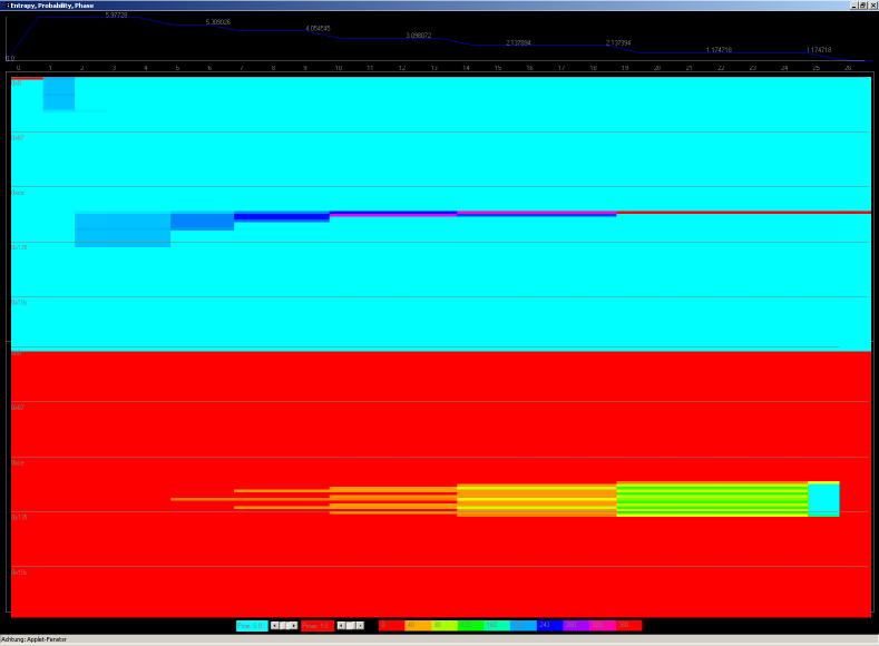
Figure 2: Simulation result for a 9 qubit Shor algorithm.

The Bloch vector $\overrightarrow{v_{i}}$ for the $i$-th qubit is given by the expectation value

$$\overrightarrow{v_{i}}=\left\langle\psi\right|\overrightarrow{\sigma}^{(i)}\left|\psi\right\rangle$$

in the notation above.

Before we close this section we will remark that the Hamiltonian above will be extended to more realistic cases like NMR by adding a periodic term in the matrix $E_{i}^{(1)}$. Furthermore we remark that the structure of the Hamiltonian above includes also all interesting cases known from condensed matter physics. There, the electron creation $a^{+}$ and annihilation $a$ operators are needed. With the settings $a^{+}=(\sigma_{x}-i\sigma_{y})/2$ and $a=(\sigma_{x}+i\sigma_{y})/2$ one can formulate a substitute of the model in terms of the Hamiltonian (3).

Example: Shor algorithm

Here we will describe the output of the Shor algorithm for the number $N=899$ with the random number $a=11$ (see Figure 2). The starting point is the division of all qubits into two registers: the $x$-register $\left|x\right\rangle$ and the $y$-register $\left|y\right\rangle$ where the length $n_{x}$ of the $x$-register is at least twice the length $n_{y}=n_{x}/2$ of the $y$-register. In this case we need $n_{y}=10$ qubits for the $y$-register encoding the number $N=899$ and at least $n_{x}=20$ qubits for the $x$-register giving 30 qubits for the whole circuit. Here we use the full capacity of the simulator with 31 qubits. At first (time step 1) we construct a Hadamard state on the $x$-register, i.e.

$$\left|x\right\rangle=\bigotimes_{i=1}^{n_{x}}\frac{1}{\sqrt{2}}\left(\left|0\right\rangle+\left|1\right\rangle\right)$$

Then we have the apply the MODULO Gate (time step 2)

$$\left|x\right\rangle\otimes\left|y\right\rangle\Rightarrow\left|x\right\rangle\otimes\left|(y\oplus(a^{x}\bmod N))\right\rangle$$

with a measurement (time step 3) of the $y$-register afterwards. Now we have an entanglement between both registers, as can be seen by the vanishing of some Bloch vectors. Beginning with time step 4, the quantum Fourier transformation “removes” all unnecessary states by interference and we are left with one state with high probability and a lot of states with low probability. Thus after the measurement of the $x$ register the algorithm is finished. A short look into the Bloch vector of the $x$-register shows the value $M=954733$. A continuous fraction expansion leads to the fraction represented by $[10,5,1,3,9,1,6,3]$ and we obtain for the proposed value of the exponent $r=7$. Only factors of this value are the solution and in our case

$$11^{210}\bmod 899=869$$

Finally we are looking for the greatest common divisors (gcd)

$$gcd(869-1,899)=31$$

$$gcd(869+1,899)=29$$

and we obtain the factors $29$ and $31$ of the number $899$.

The Figure 2 visualizes the main base states and their phases as well as the entropy of the states of a 9 qubit Shor algorithm with a 6 qubit x register and a 3 qubit y register. The problem is the factorization of $N=6$ with a random number $a=4$. We have done the simulation also for a 31 qubit Shor algorithm. The results look similar, but possess a huge number of base states, which are too many for a instructive visualization. After the first time step the entropy increases to the size of the x register, and we obtain all possible base states. Then the modulo gate mixes these states with the states of y register, and the measurement thins out some of them. Beginning with time step 4, the most interesting part starts – the quantum Fourier transformation. During this process the number of interesting base states decreases and we finish with only one state with a high probability and many states of low probability.

IV Quantum Investigations at the Internet Cafe

We have seen that the Fraunhofer Quantum Computing Service is characterized by three decisive aspects: it is a web-based computing service, it combines a simulator with a collaborative workspace, and it has a modular, extensible, and open software design. In the following let us discuss each aspect and its potentials for future developments.

The web-based design gives the simulator a ubiquitous availability. There is no need to install any software or to buy special hardware, the computing service makes quantum investigations feasible everywhere – at the institute, at home or even at the Internet cafe. All simulation runs are stored at the server and can be accessed everywhere and anytime. Especially this advantage could be a source of mistrust: the own ideas and investigations should stored on a foreign server? This sensitive aspect has to be justified by strong security protocols and high privacy standards. Each simulation job has to be encoded and unambiguously signed by owner and date making the authorship pursuable.

Closely connected to this point is the collaborative aspect of the portal. The central availability, publishing and discussion of the newest research data and documents is a key element of scientific success. The integrated content management system of the portal supports all appropriate forms of collaborative work like publishing with and without review, discussion groups, news, wiki systems etc. The quantum circuits and simulation results can be exchange by the uniform QML document format.

An important feature of the QML-based data definition is its hypertext ability. QML files with well-tried quantum circuits can be stored on any web server building a library of established modules of quantum algorithms. This modules can be included as sub-circuits in other QML files by a simple HTML reference. This facilitates the self-organized formation of a public library of quantum algorithms by the community.

This community-based building of a library of quantum circuits can be supplemented by an establishment of a network of simulation servers. The modular design of the simulation engines provides an easy way for integration of already used simulation software developed by other research groups. The requirements to integrate other simulators in our system are very low. The software has to be extended by a QML parser which will realize a common interface for all various simulators. Then, the new QML-capable engine could be run at our cluster providing a new computing service for the community. But it is also possible to install a small Java-server on the cluster of the partner group dispatching all simulation jobs which requesting the new engine. The user will not see this infrastructure details, he will only note that the portal offers more and more simulation features which are provided by more and more research groups of the community. Currently we start a cooperation with the quantum computing group at the University of Newcastle to integrate group-theoretical quantum algorithms.

We hope that our simulator and workspace will become a useful tool for the community and we will get many user responses and comments which help us to stabilize, improve and extent the system leading to the one objective of our intension: to support all efforts which brings the quantum computer from dream to reality.

V Acknowledgement

This work is supported by the German Federal Ministry of Education and Research, and we thank Marius van der Meer for facilitating the EIQU Project (FZK: 01IBB01A). We thank the group of Thomas Beth, especially Dominik Janzing, for fruitful discussions, and Uwe Der for his hard effort and deep support to bring the cluster running. Our special thank goes to Stefan Jähnichen – without whose great dedication this project would never have been started.

References

- plo (2004) Plone/Zope, http://plone.org and http://zope.org (2004).
- Trotter (1959) H. Trotter, Proc. Am. Math. Soc 10, 545 (1959).
- Suzuki (1977) M. Suzuki, Comm. Math. Phys. 57, 193 (1977).
- Golub and van Loan (1996) G. H. Golub and C. F. van Loan, Matrix Computations (The Johns Hopkins University Press, Baltimore, 1996).
- Kosloff and Kosloff (1983) R. Kosloff and D. Kosloff, J. Chem. Phys. 79, 1823 (1983).
- Horbatsch (1984) M. Horbatsch, J. Phys. B 17, 2591 (1984).
- Flocard et al. (1978) H. Flocard, S. Koonin, and M. Weiss, Phys. Rev. C 17, 1682 (1978).
- Grün et al. (1982) N. Grün, A. Müllhans, and W. Scheid, J. Phys. B 15, 4043 (1982).
- Negele (1982) J. Negele, Rev. Mod. Phys. 54, 913 (1982).
- Kosloff and Cerjan (1984) R. Kosloff and C. Cerjan, J. Chem. Phys. 81, 3722 (1984).
- Spence (1981) J. Spence, Experimental High-Resolution Electron Microscopy (Clarendon Press, Oxford, 1981).
- Feit and Fleck Jr. (1980) M. Feit and J. Fleck Jr., Appl. Opt. 19, 1154ff,2240ff,3140ff (1980).
- Kramer et al. (1981) B. Kramer, A. MacKinnon, and D. Weaire, Phys. Rev. B 23, 6357 (1981).
- Doll and Gubernatis (1990) J. Doll and J. Gubernatis, eds., Quantum Simulations (World Scientific, Singapore, 1990).
- De Raedt et al. (2000) H. De Raedt, A. Hams, K. Michielsen, and K. De Raedt, Comp. Phys. Comm. 132, 94 (2000).
- De Raedt (1987) H. De Raedt, Computer Phys. Rep. 7, 1 (1987).