Fermionic concurrence in the extended Hubbard dimer

Abstract

In this paper, we introduce and study the fermionic concurrence in a two-site extended Hubbard model. Its behaviors both at the ground state and finite temperatures as function of Coulomb interaction $U$ (on-site) and $V$ (nearest-neighbor) are obtained analytically and numerically. We also investigate the change of the concurrence under a nonuniform field, including local potential and magnetic field, and find that the concurrence can be modulated by these fields.

I Introduction

Recently, many efforts have been devoted to the entanglement in strongly correlated systemsKMOConnor2001 ; MCArnesen2001 ; XWang_PRA_64_012313 ; VSubrahmanyam04 ; SJGurecent ; AOsterloh2002 ; TJOsbornee ; Shi ; GVidal2003 ; OFSylju03 ; SJGu03 ; JVidal04 ; JSchliemann_PRA ; PZanardi_PRA_65_042101 ; JWang03 ; SJGurecent1 , in the hope that its non-trivial behavior in these systems may shed new lights on the understanding of physical phenomena of condensed matter physics. A typical case is the relation of entanglement to quantum phase transitionAOsterloh2002 ; TJOsbornee ; Shi ; GVidal2003 ; OFSylju03 ; SJGu03 ; JVidal04 . For example, Osterloh el al.,AOsterloh2002 reported that the entanglement shows scaling behavior in the vicinity of quantum phase transition point of the transverse-field Ising model. Most of previous works are for spin 1/2 systems, where the degrees of freedom at each site (or qubit) is 2. For these systems, the entanglement of formation, i.e., the concurrenceWKWootters98 , is often used as a measure of pairwise entanglement between two qubits. Such measure is only valid for $2\otimes 2$ systems. If the degrees of freedom at each qubit is larger than 2 (for example, the spin 1 system or systems consisting of fermions with spin), how to quantity the entanglement of arbitrary entangled state is a challenging issue. Several studies APeres96 ; GVidal02 ; FVerstraete04 ; FMintert04 were devoted to this issue. For example, Mintert et al. obtained a lower bound for the concurrence of mixed bipartite quantum states in arbitrary dimensions. Nevertheless, it is still very difficult to provide a reliable measure for the pairwise entanglement of systems with the number of local states larger than 2. To the best of our knowledge, none of previous work investigated the pairwise entanglement for systems consisting of electrons with spin, such as the Hubbard model, although there were a few works studied the local entanglement of fermionic models PZanardi_PRA_65_042101 ; SJGurecent1 ; JWang03 .

In this paper, we introduce and study the fermionic concurrence by using the extended Hubbard dimer as an example. Besides its importance in exploring many-body correlation in condensed matter physics, a dimer system also has potential utility in the design of quantum deviceSHill03 . By considering the Pauli’s principle, we first illustrate how to quantify the fermionic concurrence in the Hubbard model and formulate it in terms of fermion occupation and correlation so one can easily calculate it. Then based on the exact solution of the Hubbard dimer, we obtain the result at the ground state and show that the fermionic concurrence could be used to distinguish state exhibiting charge-density correlation from state exhibiting spin-density correlation. We also study its behavior at finite temperatures MCArnesen2001 , and find that it is a decreasing function of temperature. Moreover, we investigate the behavior of the concurrence under a nonuniform local potential and magnetic field GLagmago2002 ; YSun03 ; GFZhang2003 . We find that the concurrence could be modulated by these local fields. Our work therefore not only provides a possible way to investigate the pairwise entanglement in the electronic system, but also enriches our physical intuition on the systems with both charge and spin degree of freedom. Some results are instructive for future experiments.

II The model and formulism

The Hamiltonian of the one-dimensional extended Hubbard model reads

$$H=-t\sum_{\sigma,j,\delta}c^{\dagger}_{j,\sigma}c_{j+\delta,\sigma}+U\sum_{j}n_{j\uparrow}n_{j\downarrow}+V\sum_{j}n_{j}n_{j+1}.$$ (1)

where $\sigma=\uparrow,\downarrow;\,j=1,\dots,L;\delta=\pm 1$, $c^{\dagger}_{j\sigma}$ and $c_{j\sigma}$ create and annihilate an electron of spin $\sigma$ at site $j$, respectively, and the hoping amplitude $t$ is set to unit. At each site, there are four possible states, $|0\rangle_{j},\,|\uparrow\rangle_{j},\,|\downarrow\rangle_{j},\,|\uparrow\downarrow\rangle_{j}$ denoted by $|\nu\rangle_{j},\,\nu=1,2,3,4$. The Hilbert space of $L$-site system is of $4^{L}$ dimension, and $|\nu_{1},\,\nu_{2}\,\cdots\nu_{L}\rangle=\prod_{j=1}^{L}|\nu_{j}\rangle_{j}$ are its natural bases. Therefore any state in such a system can be expressed as a superposition of the above bases. We consider reduced density matrix $\rho_{jl}={\rm Tr}_{jl}\rho$ of site $j$ and $l$, where $\rho$ is the thermal density matrix of the system, and ${\rm Tr}_{jl}$ stands for tracing over all sites except the freedom of $j$th and $l$th site. Thus $\rho_{jl}$ defines the quantum correlation between site $j$ and site $l$. However, since there does not exist a well-defined entanglement measurement for a mixed state of $4\otimes 4$ bipartite systems, it is impossible to study the entanglement between two sites exactly. Fortunately, the Hilbert space of site $j$ and $l$ can be expressed in a direct-product form of electrons with spin up and spin down, that is, for site $j$ and $l$, we have two subspaces, one with the bases $|0,0\rangle,|0,\uparrow\rangle,|\uparrow,0\rangle,|\uparrow,\uparrow\rangle$, and the other one with $|0,0\rangle,|0,\downarrow\rangle,|\downarrow,0\rangle,|\downarrow,\downarrow\rangle$, respectively. It is therefore possible to investigate the problem in a given sector with spin up or spin down separately. For convenience, we restrict our studies in the subspace of spin up electrons, and the other part can be simply obtained via the $Z_{2}$ symmetry. The Hamiltonian (1) possesses U(1)$\times$SU(2) symmetry, i.e., it is invariant under the gauge transformation $c_{j,\sigma}\rightarrow e^{i\theta}c_{j,\sigma}$ and spin rotation $c_{j,\sigma}\rightarrow U_{\sigma\delta}c_{j,\delta}$, which manifest the charge and spin conservation. The latter implies the absence of coherent superposition between configurations with different eigenvalues of $n_{j,\uparrow}+{n_{j+1,\uparrow}}$. Thus the reduced density of electrons with spin-up on two sites has the form

$$\rho_{j,l}=\begin{pmatrix}u^{+}&0&0&0\\ 0&w_{1}&z&0\\ 0&z^{*}&w_{2}&0\\ 0&0&0&u^{-}\end{pmatrix}$$ (2)

in the standard bases $|0,0\rangle,|0,\uparrow\rangle,|\uparrow,0\rangle,|\uparrow,\uparrow\rangle$. Elements in the density matrix $\rho_{jl}$ are related to single occupation and correlations between the two sites,

$$z=\langle c_{j,\uparrow}^{\dagger}c_{l,\uparrow}\rangle,$$

$$u^{-}=\langle n_{j,\uparrow}n_{l,\uparrow}\rangle,$$

$$w_{1}=w_{2}=\langle n_{j,\uparrow}\rangle-\langle n_{j,\uparrow}n_{j+1,\uparrow}\rangle,$$

$$u^{+}=1-2\langle n_{j,\uparrow}\rangle+\langle n_{j,\uparrow}n_{j+1,\uparrow}\rangle.$$ (3)

where $\langle\rangle$ denotes the expectation value of the corresponding operator.

We use the concurrence as a measure of entanglement for such two-qubit system. It is defined in terms of the spectrum of the matrix $\rho_{jl}\tilde{\rho}_{jl}$WKWootters98 where $\tilde{\rho}_{jl}=\sigma^{y}_{j}\otimes\sigma_{l}^{y}\rho_{jl}^{*}\sigma_{j}^{y}\otimes\sigma^{y}_{l}$. Precisely, if $\lambda_{i}$s are eigenvalues of $\rho_{jl}\tilde{\rho}_{jl}$ and $\lambda_{1}\geq\lambda_{2}\geq\lambda_{3}\geq\lambda_{4}$, the concurrence can then be calculated as

$$C=\max\left[0,\sqrt{\lambda_{1}}-\sqrt{\lambda_{2}}-\sqrt{\lambda_{3}}-\sqrt{\lambda_{4}}\right].$$ (4)

Since there exists a monotonous relation between the concurrence and the entanglement of formation $E_{f}$, $E_{f}=-x\log_{2}x-(1-x)\log_{2}(1-x)$, where $x=1/2+\sqrt{1-C^{2}}/2$ WKWootters98 , we will hereafter use the concurrence instead of entanglement of formation in our study. From Eq. (2), the fermionic concurrence can be calculated as

$$C=2\max\left\{|\langle c_{j,\uparrow}^{\dagger}c_{l,\uparrow}\rangle|-\langle n_{j,\uparrow}n_{l,\uparrow}\rangle,\;0\right\}$$ (5)

III Hubbard dimer with two electrons

In this section, we consider a model which consists of two sites and two electrons, because not only can it be exactly solved, but also it gives us a clear physical picture. The Hamiltonian for the dimer reads

$$H = -2\sum_{\sigma}(c^{\dagger}_{1,\sigma}c_{2,\sigma}+c^{\dagger}_{2,\sigma}c_{1,\sigma})$$ (6)

$$+U(n_{1,\uparrow}n_{1,\downarrow}+n_{2,\uparrow}n_{2,\downarrow})+2Vn_{1}n_{2}.$$

In the standard bases $|\uparrow,\downarrow\rangle,|\downarrow,\uparrow\rangle,|\uparrow\downarrow,0\rangle,|0,\uparrow\downarrow\rangle$ of the reduced subspace with zero magnetization: $S^{z}=0$, $H$ is a $4\times 4$ matrix

$$H=\begin{pmatrix}U&0&-2&-2\\ 0&U&-2&-2\\ -2&-2&2V&0\\ -2&-2&0&2V\end{pmatrix},$$ (7)

and we can easily obtain its eigenfunction

$$\Psi_{1}=\frac{\sin\theta}{\sqrt{2}}\left[|\uparrow\downarrow,0\rangle+|0,\uparrow\downarrow\rangle\right]+\frac{\cos\theta}{\sqrt{2}}\left[|\uparrow,\downarrow\rangle+|\downarrow,\uparrow\rangle\right]$$

$$\Psi_{2}=\frac{\cos\theta}{\sqrt{2}}\left[|\uparrow\downarrow,0\rangle+|0,\uparrow\downarrow\rangle\right]-\frac{\sin\theta}{\sqrt{2}}\left[|\uparrow,\downarrow\rangle+|\downarrow,\uparrow\rangle\right]$$

$$\Psi_{3}=\frac{1}{\sqrt{2}}\left[|\uparrow\downarrow,0\rangle-|0,\uparrow\downarrow\rangle\right]$$

$$\Psi_{4}=\frac{1}{\sqrt{2}}\left[|\uparrow,\downarrow\rangle-|\downarrow,\uparrow\rangle\right]$$ (8)

where $\theta$ is defined as

$$\tan\theta=\frac{4}{(U/2-V)+\sqrt{(U/2-V)^{2}+16}}.$$

The corresponding eigenvalues are

$$E_{1}=\frac{1}{2}(U+2V-\sqrt{64+(U-2V)^{2}}),$$

$$E_{2}=\frac{1}{2}(U+2V+\sqrt{64+(U-2V)^{2}}),$$

$$E_{3}=U,$$

$$E_{4}=2V.$$ (9)

¿From the ground-state wavefunction, we have

$$\langle c^{\dagger}_{1,\uparrow}c_{2,\uparrow}\rangle = \sin\theta\cos\theta$$

$$\langle n_{1,\uparrow}n_{2,\uparrow}\rangle = 0.$$ (10)

Thus, the fermionic concurrence takes the form of

$$C=|\sin 2\theta|.$$ (11)

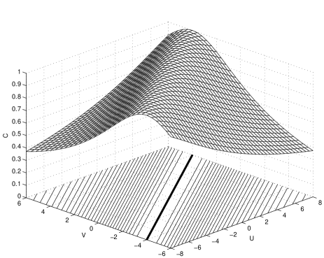
Figure 1: The fermionic concurrence of the extended Hubbard dimer as a function of $U$ and $V$. The curves in the $C=0$ plane constitutes a contour map, and the thick line denotes the local extremum.

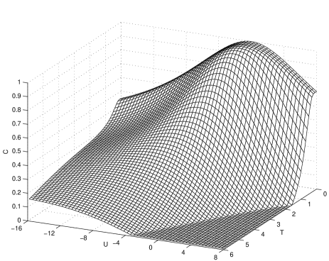
Figure 2: The fermionic concurrence of the Hubbard dimer ($V=0$) as a function of $U$ and $T$.

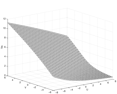
Figure 3: The threshold temperature $T_{th}$ of the fermionic concurrence as a function of $U$ and $V$.

Clearly, the ground-state wavefunction simultaneously comprises the states of the double occupied state $|\uparrow\downarrow,0\rangle+|0,\uparrow\downarrow\rangle$ and the single occupied state $|\uparrow,\downarrow\rangle+|\downarrow,\uparrow\rangle$. The magnitude of $\theta$ determines which of them dominates in the ground state. From its definition, it is easy to learn that the line $U=2V$, i.e. $\theta=45^{\circ}$, separates the two regions. One region dominated by $|\uparrow\downarrow,0\rangle+|0,\uparrow\downarrow\rangle$ corresponds to the charge-density-wave state for a large system, and the other one dominated by $|\uparrow,\downarrow\rangle+|\downarrow,\uparrow\rangle$ corresponds to the spin-density-wave state. Clearly, the fermionic concurrence reaches a maximum at the line $V=U/2$, and shows the mirror symmetry along the line $V=U/2$ (See figure 1).

At finite temperatures, the expectation value of a given operator $O$ is $\langle O\rangle=\sum_{n}\langle n|O|n\rangle e^{-\beta E_{n}}/Z$, where $\beta=1/T$, $Z$ is the partition function, and $E_{n}$ denotes the energy spectra. For the present model, we should also take into account states in the subspace with $S^{z}=\pm 1$ besides that of $S^{z}=0$. Then we have two additional states $\Psi_{5(6)}=|\uparrow,\uparrow\rangle(|\downarrow,\downarrow\rangle)$ with the same eigenvalue $E_{5(6)}=2V$. Thus the fermionic concurrence of the Hubbard dimer takes the form,

$$C(T)=\frac{1}{Z}\max\left[|\sin 2\theta(e^{-\beta E_{1}}-e^{-\beta E_{2}})|-2e^{-\beta E_{5}},\,0\right].$$ (12)

It is not difficult to prove that the above expression is a decreasing function of $T$, as shown in figure 2 for a specific value of $V=0$.

In the high temperature limit, $T\rightarrow\infty$, the Boltzmann weight of each eigenstate becomes almost equal, so the first term in the square brackets of Eq. (12) becomes negative and we have a vanishing fermionic concurrence. Hence we expect that there exists a threshold temperature $T_{\rm th}$ at which the concurrence becomes zero. Precisely, it is determined by

$$\left|\sin 2\theta(e^{-E_{1}/T_{\rm th}}-e^{-E_{2}/T_{\rm th}})\right|-2e^{-E_{5}/T_{\rm th}}=0.$$ (13)

Clearly, the hoping-correlation $\langle c_{j,\uparrow}^{\dagger}c_{l,\uparrow}\rangle$ arises from the state of $\Psi_{1}$ and $\Psi_{2}$, and charge correlation $\langle n_{1,\uparrow}n_{2,\uparrow}\rangle$ from $\Psi_{5}$. Since the Boltzmann weight $e^{-E_{1}/T_{\rm th}}$ of $\Psi_{1}$ is always larger than $e^{-E_{2}/T_{\rm th}}$, the term of absolute value is then positive for finite $T$. However, the term $U+2V$ in the expression of Boltzmann wight breaks the mirror symmetry of the fermionic concurrence at the ground-state along the line $U=2V$. For example, the concurrence in the fourth quadrant of the $U-V$ plane is more susceptive to thermal fluctuation and might be easily suppressed to zero than other quadrants. Therefore, in different quadrants, the effect of thermal fluctuation is quite different. Then from Eq. (13), we obtain a slope-like threshold temperature for the concurrence (see figure 3).

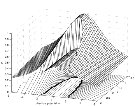
Figure 4: The fermionic concurrence as a function of the local potential $\mu$ ($u$ instead of $\mu$ as an indictor for axes) and V at the ground-state. Here, $U=2$.

IV Under a nonuniform field

In this section, we would like to consider the behavior of the concurrence under an external field. In general, a uniform external field, like the local potential or the magnetic field, suppresses the concurrence since it frustrates the hoping process. Thus we are only interested in the case with a nonuniform field. Moreover, differing from the previous investigation where calculations were done for canonical ensembles, we perform calculation for grand canonical ensembles. The first case we consider is to add site energy term to the Hamiltonian (6)

$$H_{\mu}=\mu_{1}(n_{1,\uparrow}+n_{1,\downarrow})+\mu_{2}(n_{2,\uparrow}+n_{2,\downarrow}).$$ (14)

For simplicity, we set $\mu=\mu_{1}=-\mu_{2}$, since the main physics is not changed under this condition.

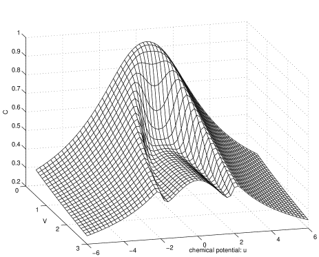
Figure 5: The fermionic concurrence as a function of chemical potential $\mu$ ($u$ instead of $\mu$ as an indictor for axes) and V at $T=0.1$. Here $U=2$.

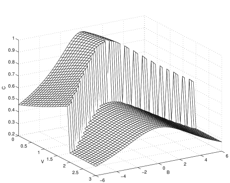
Figure 6: The fermionic concurrence as a function of magnetic field $B$ and V at the ground-state. Here $U=2$.

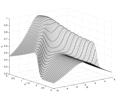
Figure 7: The fermionic concurrence as a function of magnetic field $B$ and V at $T=0.1$. Here $U=2$.

We show the fermionic concurrence as a function of $\mu$ and $V$ as well as its corresponding contour map in the ground-state for a specific value of $U=2$ in Fig. 4. Clearly the ground-state phase diagram can be obtained from the contour map. The area outside the arc is the spin singlet state described in Eq. (8), while the inside area is one-particle state. Thus the arc in the contour-map is just the level crossing point for different states. The level-crossing also leads to a jump on the surface of the concurrence in the $\mu-V$ plane. Since the experiments are always done at finite temperatures, it is useful to investigate the effect of thermal fluctuation. We show the dependence of the fermionic concurrence on $\mu$ and $V$ at $T=0.1$ in Fig. 5 where we observe that the jump at the level-crossing point in Fig. 4 is eliminated by the thermal fluctuation. We find, at some points, eg., $U=2$ and $V=1$, the concurrence is small when $\mu=0$. If we change the value of $\mu$ the thermal concurrence can be increased substantially. Such a role played by the local potential is important, because the change of $\mu$ in principle can be realized by the electric field so it provides a possible way to control the magnitude of the concurrence.

The second case we consider is to add a Zeeman-like term to the Hamiltonian (6)

$$H_{Zee}=-B_{1}(n_{1,\uparrow}-n_{1,\downarrow})/2-B_{2}(n_{2,\uparrow}-n_{2,\downarrow})/2.$$ (15)

For simplicity, we again set $B=B_{1}=-B_{2}$. We show the concurrence as a function of $B$ and $V$ for a specific value of $U=2$ in the ground state in Fig. 6, and at $T=0.1$ in Fig. 7, respectively. Similar to the first case, the magnetic field may also induce the level-crossing in the ground-state, which may lead to a quantum phase transition. The induced level-crossing results in a jump on the surface of the concurrence in the $B-V$ plane. Such a jump is blurred by the thermal fluctuation, as shown in Fig. 7. Here we have an interesting phenomena: although the fermionic concurrence is defined in a single sector, such as for spin-up electrons only, it can still be modulated by the other sector (spin-down electron) through magnetic field. For the present case, the magnetic field does not always decrease the concurrence, it may actually increase the concurrence in some regions. Therefore, a nonuniform magnetic field can be in favor of the entanglement of formation between two qubits.

V summary and acknowledgement

In summary, we first presented a possible way to study the concurrence as a measure of pairwise entanglement for fermionic systems. Then we studied its behavior in the Hubbard dimer both at zero and finite temperatures. It was interesting to observe that the classification of two different regions, one dominated by the charge-density correlation $[|\uparrow\downarrow,0\rangle+|0,\uparrow\downarrow\rangle]$ while the other one dominated by the spin-density correlation $[|\uparrow,\downarrow\rangle+|\downarrow,\uparrow\rangle]$, is closely related to the behavior of the fermionic concurrence at the ground state. At finite temperatures, we also obtained the explicit expression of $C$ for general $U$ and $V$, and found that it is a decreasing function of the temperature, which leads to a condition of the threshold temperature where the concurrence vanishes. We then obtained the threshold temperature as a function of $U$ and $V$ numerically. Our method, as we pointed out in the introduction, could be easily extended to other electronic systems. Results obtained in this paper help us gain more insight into physical properties of strongly correlated systems. Moreover, we studied the role of nonuniform local potential as well as magnetic field for the extended Hubbard dimer. We found that both of them can be used to modulate the concurrence. Though our analysis is based on a specific value of $U=2$, the main physics is the same for other positive $U$. Finally, we want to point out that although results obtained in this paper are for a 2-site (dimer) system, their qualitative features should be the same for big size system.

This work is supported by the Earmarked Grant for Research from the Research Grants Council (RGC) of the HKSAR, China (Project No 401703). We thank Prof. G. S. Tian for many helpful discussions.

References

- (1) K. M. O’Connor and W. K. Wootters, Phys. Rev. A 63, 052302 (2001).
- (2) M. C. Arnesen, S. Bose, and V. Vedral, Phys. Rev. Lett 87, 017901(2001).
- (3) X. Wang, Phys. Rev. A 64, 012313 (2001); X. Wang, Phys. Rev. A 66, 034302 (2002); X. Wang, Phys. Rev. A 66, 044305 (2002).
- (4) V. Subrahmanyam, Phys. Rev. A 69, 022311 (2004).
- (5) S. J. Gu, H. Li, Y. Q. Li, H. Q. Lin, quant-ph/0403026 (unpublished).
- (6) A. Osterloh, Luigi Amico, G. Falci and Rosario Fazio, Nature 416, 608 (2002).
- (7) T. J. Osborne and M.A. Nielsen, Phys. Rev. A 66, 032110 (2002).
- (8) Y. Shi, Phys. Lett. A 309, 254 (2003).
- (9) G. Vidal, J. I. Latorre, E. Rico, and A. Kitaev, Phys. Rev. Lett. 90, 227902 (2003).
- (10) O. F. Syljuåsen Phys. Rev. A 68, 060301 (2003).
- (11) S. J. Gu, H. Q. Lin, and Y. Q. Li, Phys. Rev. A 68, 042330 (2003).
- (12) J. Vidal, G. Palacios, and R. Mosseri, Phys. Rev. A 69, 022107 (2004); J. Vidal, R. Mosseri, and J. Dukelsky, Phys. Rev. A 69, 054101 (2004).
- (13) J. Schliemann, J. I. Cirac, M. Kus, M. Lewenstein, and D. Loss, Phys. Rev. A 64, 022303 (2001).
- (14) P. Zanardi, Phys. Rev. A 65, 042101 (2002); P. Zanardi and X. Wang, J. Phys. A: Math. Gen. 35, 7947 (2002).
- (15) J. Wang, and S. Kais, Int. J. Quant. Information 1, 375 (2003).
- (16) S. J. Gu, S. S. Deng, Y. Q. Li, H. Q. Lin, quant-ph/0405067 (unpublished).
- (17) W. K. Wootters, Phys. Rev. Lett. 80, 2245 (1998); S. Hill and W. K. Wootters Phys. Rev. Lett. 78, 5022 (1997).
- (18) A. Peres, Phys. Rev. Lett. 77, 1413 (1996).
- (19) G. Vidal, and R. F. Werner, Phys. Rev. A 65, 032314 (2002).
- (20) F. Verstraete, M. Popp, and J. I. Cirac, Phys. Rev. Lett. 92, 027901 (2004); F. Verstraete, M. A. Martín-Delgado, and J. I. Cirac, Phys. Rev. Lett. 92, 087201 (2004).
- (21) F. Mintert, M. Kuś, and A. Buchleitner, Phys. Rev. Lett. 92, 167902 (2004).
- (22) S. Hill, R. S. Edwards, N. Aliaga-Alcalde, G. Christou, Science 302, 1015 (2003).
- (23) G. L. Kamta and Anthony F. Starace, Phys. Rev. Lett. 88, 107901 (2002).
- (24) Y. Sun, Y. Chen, and H. Chen, Phys. Rev. A 68, 044301 (2003).
- (25) G. F. Zhang, J. Q. Liang, and Q. W. Yan, Chin. Phys. Lett. 20, 452 (2003).