Resonances for coupled Bose-Einstein Condensates

Abstract

We study some effects arising from periodic modulation of the asymmetry and the barrier height of a two-well potential containing a Bose-Einstein condensate. At certain modulation frequencies the system exhibits resonances, which may lead to enhancement of the tunneling rate between the wells and which can be used to control the particle distribution among the wells. Some of the effects predicted for a two-well system can be carried over to the case of a Bose-Einstein condensate in an optical lattice.

I Introduction

Since the experimental realization of Bose-Einstein condensates (BEC) one has considered the possibility of extending one-mode models to two or more modes [1]. This raises the issue of the relative phase between modes. As indicated by several authors [2], a two-well BEC may exhibit features that are not covered by the semiclassical description in terms of the Gross-Pitaevski equation. These features are significant at low particle numbers and for strong interactions. In previous work, we discussed some aspects of the dynamics of a two-well BEC in the strong-interaction regime [3]. This is close to the experimental situation for a BEC in a double-well trap, designed in Ref. [4].

A sensitive way to probe the properties of a BEC in a double-well potential with strong interatomic interactions is to look for resonant behavior when a parameter of the system is periodically modulated. The response of the system may be expected to be very sensitive to the value of the modulation frequency in the neighborhood of a resonance. A periodic perturbation can be implemented in various ways. One example would be periodically modulating the trapping potential. Salmond et al [5] study a numerical model of a double-well potential with periodically modulated coupling between the wells. This semiclassical analysis reveals the existence of uncoupled regions with chaotic and regular motion. The inclusion of the quantum nature of the evolution leads to transitions between these regions. Another type of periodic perturbation can be imposed by periodically modulating the energy difference between the ground states in the two wells.

Periodic modulations are known to give rise to dynamical localization in some cases. This effect has been widely discussed in the literature in the case a particle in a periodic potential, such as an electron in a crystal or an atom in an optical lattice [6] and [7]. When the particle also feels a uniform force in addition to the lattice potential (a tilted optical lattice), it is found to have an infinite discrete set of equidistant energy levels, with a level separation that is determined by the strength of the uniform force [7]. A variation of the magnitude of the uniform force affects the phase of the state. So, when this magnitude is periodically modulated, resonances may be expected. The population in one well is described by adding the amplitudes for arriving at this well from various other wells, each one with a different phase shift. In the long time limit, when the time of observation is long compared to the period of the modulation, this gives rise to destructive interference, leading to a suppression of the net tunneling rate. Hence, the asymptotic distribution over the wells coincides with the initial one, and dynamical localization has been realized.

Another example of dynamical localization arises for a single two-level atom in a driving field with a periodically modulated detuning [8]. For certain ratios of the modulation frequency and the strength of the field, the atom is localized in its ground state. The time scale is restricted by the modulation frequency.

In the present case of a BEC in a two-well potential with a fixed total number of atoms, the state space is finite dimensional. In the SU(2) representation of the operator algebra, the Hamiltonian has a quadratic term due to the interatomic interactions. So, in this sense the system is quite different from that of an atom in a tilted lattice, with its infinite number of states and a Hamiltonian that is linear in the SU(2) operators. Still, there are some obvious similarities: the discrete structure of the energy and the presence of interatomic interactions and tunneling between wells as competing processes. Therefore, we expect interesting effects also in the two-well case when the energy difference or the hopping between wells is periodically modulated. From a formal point of view, the analysis in the present paper may be regarded as a generalization of the process of dynamical localization for the Hamiltonian with a quadratic term. Specifically, this paper considers the possibilites of coherent control of a BEC in a double-well potential by using any kind of time-periodic perturbation.

II BEC in a double potential well

We describe a BEC in a double potential well in terms of a one-particle Hamiltonian $H^{(1)}$ and a two-particle interaction $U({\vec{r}},{\vec{r}}^{\prime})$. The states $\left|1\right\rangle$ and $\left|2\right\rangle$ are the the localized ground states in either well, with wave functions $\psi_{1}({\vec{r}})$ and $\psi_{2}({\vec{r}})$. On the basis of the states $\left|1\right\rangle$ and $\left|2\right\rangle$, the one-particle Hamiltonian has the matrix elements

$$\left\langle 1\right|H^{(1)}\left|1\right\rangle=-\left\langle 2\right|H^{(1)}\left|2\right\rangle=\hbar\varepsilon/2,\left\langle 1\right|H^{(1)}\left|2\right\rangle=\left\langle 2\right|H^{(1)}\left|1\right\rangle=-\hbar\delta/2\;.$$ (1)

In the case that $\varepsilon=0$, the coupling between the wells lifts their degeneracy, and creates an energy splitting $\hbar\delta$ between the even ground state $\left|g\right\rangle$ and the odd excited state $\left|e\right\rangle$, defined by

$$\left|g\right\rangle=\frac{1}{\sqrt{2}}(\left|1\right\rangle+\left|2\right\rangle);\;\left|e\right\rangle=\frac{1}{\sqrt{2}}(\left|1\right\rangle-\left|2\right\rangle)\;.$$ (2)

When we restrict ourselves to these two states, the field operator in second quantization has the standard form

$$\widehat{\Psi}(\overrightarrow{r})=\widehat{a}_{1}\psi_{1}({\vec{r}})+\widehat{a}_{2}\psi_{2}({\vec{r}}),$$ (3)

with $\widehat{a}_{i}$ the one-particle annihilation operator in the two states, which together with the corresponding creation operators obey the bosonic commutation rules. When we substitute this expression in the formal expression

$$\widehat{H}=\int d\overrightarrow{r}\widehat{\Psi}^{\dagger}(\overrightarrow{r})H^{(1)}\widehat{\Psi}(\overrightarrow{r})+\frac{1}{2}\int d\overrightarrow{r}d\overrightarrow{r}^{\prime}\widehat{\Psi}^{\dagger}(\overrightarrow{r})\widehat{\Psi}^{\dagger}(\overrightarrow{r}^{\prime})U({\vec{r}},{\vec{r}}^{\prime})\widehat{\Psi}(\overrightarrow{r})\widehat{\Psi}(\overrightarrow{r}^{\prime}).$$ (4)

for the second-quantized Hamiltonian, we find

$$\widehat{H}=\sum_{i,k}\hbar\left\langle i\right|H^{(1)}\left|k\right\rangle\widehat{a}_{i}^{\dagger}\widehat{a}_{k}+\frac{1}{2}\sum_{i,k,l,m}\hbar\left\langle i,k\right|U\left|l,m\right\rangle\kappa_{i,k,l,m}\widehat{a}_{i}^{\dagger}\widehat{a}_{k}^{\dagger}\widehat{a}_{l}\widehat{a}_{m},$$ (5)

where the indices $i$, $j$, $k$, $l=1$ or $2$, and the matrix elements are taken between the states $\psi_{1}$ and $\psi_{2}$. .

At sufficiently low energy, the two particle interaction is well approximated by the contact potential $U({\vec{r}},{\vec{r}}^{\prime})=(4\pi\hbar^{2}a/m)\delta({\vec{r}}-{\vec{r}}^{\prime})$, with $a$ the scattering length. The function $\psi_{1}$ and $\psi_{2}$ states have the same form, and we assume that they do not overlap. So we obtain the following expression for the Hamiltonian

$$\widehat{H}=\frac{\hbar\varepsilon}{2}\left(\widehat{a}_{1}^{\dagger}\widehat{a}_{1}-\widehat{a}_{2}^{\dagger}\widehat{a}_{2}\right)-\frac{\hbar\delta}{2}\left(\widehat{a}_{1}^{\dagger}\widehat{a}_{2}+\widehat{a}_{2}^{\dagger}\widehat{a}_{1}\right)+\frac{\hbar\kappa}{2}\left(\widehat{a}_{1}^{\dagger}\widehat{a}_{1}^{\dagger}\widehat{a}_{1}\widehat{a}_{1}+\widehat{a}_{2}^{\dagger}\widehat{a}_{2}^{\dagger}\widehat{a}_{2}\widehat{a}_{2}\right).$$ (6)

where the parameter $\kappa$ defined by

$$\hbar\kappa={\frac{4\pi\hbar^{2}a}{m}}\int d{\vec{r}}\;|\psi_{1}({\vec{r}})|^{4}\;$$ (7)

measures the strength of the interatomic interaction.

For convenience we express the Hamiltonian (6) in terms of SU(2) operators by applying the standard Schwinger representation of two modes. This leads to the definition

$$\widehat{J}_{z}={\frac{1}{2}}\left(\widehat{a}_{1}^{\dagger}\widehat{a}_{1}-\widehat{a}_{2}^{\dagger}\widehat{a}_{2}\right)\;,\;\widehat{J}_{+}=\widehat{a}_{1}^{\dagger}\widehat{a}_{2}\;,\;\widehat{J}_{-}=\widehat{a}_{2}^{\dagger}\widehat{a}_{1}.$$ (8)

These operators are related to the Cartesian components of a fictitious angular momentum by the standard relations $\widehat{J}_{\pm}=\widehat{J}_{x}\pm i\widehat{J}_{y}$. They obey the commutation rules for angular momentum operators

$$[\widehat{J}_{z},\widehat{J}_{\pm}]=\pm\widehat{J}_{\pm}\;,\;[\widehat{J}_{+},\widehat{J}_{-}]=2\widehat{J}_{z}\;,$$ (9)

which generate the SU(2) algebra. These operators commute with the operator for the total number of particles $\widehat{N}=\widehat{a}_{1}^{\dagger}\widehat{a}_{1}+\widehat{a}_{2}^{\dagger}\widehat{a}_{2}$. The Hamiltonian (6) can be rewritten in the form

$$\widehat{H}=\widehat{H}_{N}+\frac{\hbar\kappa}{4}\left(\widehat{N}^{2}-2\widehat{N}\right)\;,$$ (10)

where the $N$-particle Hamiltonian $\widehat{H}_{N}$ is defined by

$$\widehat{H}_{N}=\hbar\varepsilon\widehat{J}_{z}-\hbar\delta\widehat{J}_{x}+\hbar\kappa\widehat{J}_{z}^{2}.$$ (11)

For a given number of particles $N$, the last term in Eq. (10) is a constant, and it suffices to consider the dynamics of the subspace of the $N+1$ number states $\left|n,N-n\right\rangle$, with $n=0,1,\dots N$, with $n$ particles in well $1$, and $N-n$ particles in well $2$. This subspace has the structure of the angular momentum states, with $J=N/2$, and the $2J+1$ magnetic quantum numbers $\mu=n-N/2$, with $\mu=-J,-J+1,\dots,J$. Note that $\mu$ is half the difference of the particle number in two wells. For a given particle number $N$ we represent the number states by the quantum number $\mu$, so that $\left|\mu\right\rangle\equiv\left|n,N-n\right\rangle$. The action of the operators $\widehat{J}_{0}$ and $\widehat{J}_{\pm}$ on the Fock states has the well-known behavior

$$\widehat{J}_{z}\left|\mu\right\rangle=\mu\left|\mu\right\rangle\;,\;\widehat{J}_{\pm}\left|\mu\right\rangle=\sqrt{\left(J\mp\mu\right)\left(J\pm\mu+1\right)}\left|\mu\pm 1\right\rangle.$$ (12)

This also determines the action of the Cartesian operators $\widehat{J}_{x}$ and $\widehat{J}_{y}$.

III Quantum states in two wells

The Schwinger representation of the operators occurring in the Hamiltonian suggests in a natural way various possible choices of states of $N$ atoms in the two wells. Arecchi et al [9] introduced the spin coherent states (SCS) [10], in analogy to the Glauber coherent state of a mode of the quantum radiation field. The SCS follow from applying an arbitrary rotation to the state $\left|\mu\right\rangle$ with $\mu=J$. As rotation operator we take

$$\widehat{R}(\theta,\phi)=\exp(-i\phi\widehat{J}_{z})\exp(-i\theta\widehat{J}_{y})\exp(i\phi\widehat{J}_{z})=\exp[-i\theta(\widehat{J}_{y}\cos\phi-\widehat{J}_{x}\sin\phi)],$$ (13)

which represents a rotation over an angle $\theta$, around an axis in the $xy$-plane, specified by the angle $\phi$ with the $y$-axis. The SCS $\left|\theta,\phi;J\right\rangle$ is

$$\left|\theta,\phi;J\right\rangle=\widehat{R}(\theta,\phi)\left|J\right\rangle$$ (14)

which is also the eigenstate with eigenvalue $J$ of the component $\overrightarrow{u}\cdot\widehat{\overrightarrow{J}}$ of the angular-momentum vector in the direction $\overrightarrow{u}$ specified by the polar angle $\theta$ and the azimuthal angle $\phi$. Just as the Glauber coherent states of a mode with annihilation operator $\widehat{c}$ can be obtained by acting with a displacement operator $\widehat{D}\left(\zeta\right)=$ $\exp\left(\zeta\widehat{c}^{\dagger}-\zeta^{*}\widehat{c}\right)$ on the vacuum state, the SCS follows by a rotation $\widehat{R}(\theta,\phi)=\exp\left(\zeta\widehat{J}_{-}-\zeta^{*}\widehat{J}_{+}\right)$ with $\zeta=\left(\theta/2\right)\exp\left(i\phi\right)$, acting on the state $\left|J\right\rangle$. When we view this state $\left|J\right\rangle$ as the ground state, the operator $\widehat{J}_{+}$ is analogous to the annihilation operator, since $\widehat{J}_{+}\left|J\right\rangle=0$. An essential difference between the two cases is, of course, that the state space of a radiation mode has infinite dimensions, while the dimension of the angular-momentum state space is $2J+1$.

In our case, the analogy is carried one step further, since the SCS defined by (14) do not represent angular-momentum states, but refer to the states of $N$ atoms, distributed over two potential wells. The ground state $\left|J\right\rangle$ represents the state with all particles in the first well. When we substitute the identity $\left|J\right\rangle=\left(\widehat{a}_{1}^{\dagger}\right)^{N}\left|vac\right\rangle/\sqrt{N!}$ with $N=2J$ into the right-hand side of (14), we obtain an expression for the SCS in the language of the two wells, in the form

$$\left|\theta,\phi;J\right\rangle=\frac{1}{\sqrt{N!}}\left(\cos\frac{\theta}{2}\text{ }\widehat{a}_{1}^{\dagger}+e^{i\phi}\sin\frac{\theta}{2}\text{ }\widehat{a}_{2}^{\dagger}\right)^{N}\left|vac\right\rangle.$$ (15)

We can interpret (15) as a state with $N$ atoms in the one-particle superposition state

$\displaystyle\cos\frac{\theta}{2}\text{ }\left|1\right\rangle+e^{i\phi}\sin\frac{\theta}{2}\text{ }\left|2\right\rangle$

of the two wells. A special case arises for $\theta=\pi/2$, when the average populations of the two wells are the same. Then the state (15) describes a collective mode from two interfering sources of equal intensity, and its expansion in number states is given by

$$\left|\pi/2,\phi;J\right\rangle=\frac{1}{2^{N/2}}\sum_{n=0}^{N}\left(\begin{array}[]{l}N\\ n\end{array}\right)^{1/2}e^{i\left(N-n\right)\phi}\left|n,N-n\right\rangle$$ (16)

Such a state can be considered as a state with a well-defined phase difference $\phi$. The atom distribution over the two wells is binomial, and they have been termed phase states (PS) of a two-mode boson system in Ref. [11]. For simplicity, we suppress the value $\pi/2$ in this case, and we simply denote the PS as $\left|\phi;J\right\rangle$ . Upon rotation around the $z$-axis, a PS transforms as

$$\exp(-i\alpha\widehat{J}_{z})\left|\phi;J\right\rangle=\exp(-i\alpha J)\left|\phi+\alpha;J\right\rangle$$ (17)

The concept of Glauber coherent states of a radiation mode has been generalized by de Oliveira et al [12], who introduced so called displaced coherent states defining them as a displaced number state, rather than a displaced vacuum state. The corresponding generalization of a SCS is found when the rotation operator (13) acts on a number state $\left|\mu\right\rangle$. The resulting displaced spin coherent states (DSCS) are

$$\left|\theta,\phi;\mu\right\rangle=\widehat{R}(\theta,\phi)\left|\mu\right\rangle.$$ (18)

They are the eigenstates of the angular-momentum component $\overrightarrow{u}\cdot\widehat{\overrightarrow{J}}$ with eigenvalue $\mu$. In the special case that $\theta=\pi/2$ and $\phi=0$, we find that $\widehat{R}(\theta,\phi)=\exp(-i\pi\widehat{J}_{y}/2)$, and this component is simply $\widehat{J}_{x}$. Its eigenstates are denoted as

$\displaystyle\left|\pi/2,0;\mu\right\rangle=\left|\mu\right\rangle_{x}.$

and they obey the eigenvalue relation $\widehat{J}_{x}\left|\mu\right\rangle_{x}=\mu\left|\mu\right\rangle_{x}$. The state $\left|\mu\right\rangle_{x}$ describes a state with $J+\mu$ atoms in the even state $\left|g\right\rangle$, and $J-\mu$ atoms in the odd state $\left|e\right\rangle$. These states are coupled by the ladder operators

$$\widehat{J}_{x}^{\pm}\equiv\exp(-i\pi\widehat{J}_{y}/2)\widehat{J}_{\pm}\exp(i\pi\widehat{J}_{y}/2)=-\widehat{J}_{z}\pm i\widehat{J}_{y},$$ (19)

according to the relations

$\displaystyle\widehat{J}_{x}^{\pm}\left|\mu\right\rangle_{x}=\sqrt{\left(J\mp\mu\right)\left(J\pm\mu+1\right)}\left|\mu\pm 1\right\rangle_{x}.$

When $\theta=\pi/2$ and $\phi=\pi/2$, the DSCS are indicated as

$\displaystyle\left|\pi/2,\pi/2;\mu\right\rangle=\left|\mu\right\rangle_{y},$

which are eigenstates of $\overrightarrow{u}\cdot\widehat{\overrightarrow{J}}=\widehat{J}_{y}$, as specified by the relation $\widehat{J}_{y}\left|\mu\right\rangle_{y}=\mu\left|\mu\right\rangle_{y}$. The corresponding ladder operators are

$$\widehat{J}_{y}^{\pm}\equiv\exp(i\pi\widehat{J}_{x}/2)\widehat{J}_{\pm}\exp(-i\pi\widehat{J}_{x}/2)=\widehat{J}_{x}\mp i\widehat{J}_{z}.$$ (20)

In the special case that $\mu=J$, the DSCS $\left|\mu\right\rangle_{x}$ and $\left|\mu\right\rangle_{y}$ become the SCS $\left|J\right\rangle_{x}$ and $\left|J\right\rangle_{y}$, which are also the PS with $\phi=0$ and $\phi=\pi/2$, respectively.

IV Evolution in limiting cases

For a given number $N$ of atoms, the evolution is characterized by an evolution operator that is governed by the Hamiltonian (11), and that obeys the Schrödinger equation

$$i\hbar\frac{d\widehat{U}}{dt}=\widehat{H}_{N}\widehat{U}.$$ (21)

In order to get an intuitive insight into the evolution, we first consider two extreme cases, which are simple to understand. We assume that the two wells have equal energy, so that $\varepsilon=0$. If the interatomic interactions are negligible, the quadratic term in (11) can be skipped. For a possibly time-dependent coupling strength $\delta$, the evolution operator is

$$\widehat{U}(t)=\exp\left(i\eta\left(t\right)\widehat{J}_{x}\right),$$ (22)

with $\eta\left(t\right)=\int_{0}^{t}\delta(t^{{}^{\prime}})dt^{{}^{\prime}}$ the area of the coupling pulse. In the language of angular momentum, $\widehat{U}$ represent a rotation over an angle $-\eta$ around the $x$-axis. In this case, the states $\left|\mu\right\rangle_{x}$ are eigenstates of the evolution operator, so that these states acquire only a phase factor $\exp\left(i\eta\left(t\right)\mu\right)$. An initial state in the form of a single number state $\left|\mu\right\rangle$ state gets rotated by the operator (22) and evolves into a superpostion of number states. At the instant that $\eta\left(t\right)=\pi/2$ an initial number state has evolved into an eigenstate of the operator $\widehat{J}_{y}.$

Conversely, when the interatomic interactions are strong enough on the scale of tunneling, the hopping between the wells can get suppressed [3]. Now, a single number state $\left|\mu\right\rangle$ only acquires a phase factor $\exp(-i\kappa\mu^{2}t)$. The evolution operator takes the form

$$\widehat{U}\left(t\right)=e^{-i\kappa\widehat{J}_{z}^{\text{ }2}t},$$ (23)

which cannot be conceived as a rotation in the angular-momentum space. Since the eigenvalues of $\widehat{J}_{z}^{2}$ are discrete, the evolution (23) has revivals. First we consider the situation that the number of particles $N$ is even, so that the eigenvalues $\mu$ of $\widehat{J}_{z}^{\text{ }}$ are integer. Then the eigenvalues of $\widehat{U}$ are $\exp(-i\kappa\mu^{2}t)=1$ when $t=mT$, with $m$ an integer, and $T=2\pi/\kappa$ . At these times the initial state is reproduced, which proves that the evolution of any initial state is time periodic, with period $T$. For a time $t=T/2$, which is half the period, the eigenvalues of $\widehat{U}(T/2)$ are $\exp(-i\pi\mu^{2})=(-1)^{\mu}$, which proves that the evolution operator at this instant is equal to

$\displaystyle\widehat{U}(T/2)=\exp(-i\pi\widehat{J}_{z}).$

For an initial PS $\left|\Psi(0)\right\rangle=\left|\phi;J\right\rangle$, we find that the state at the time $t=T/2$ is

$\displaystyle\left|\Psi(T/2)\right\rangle=\exp(-i\pi J)\left|\phi;J\right\rangle,$

which is just the opposite PS. At other instants of time, that are a simple rational fraction of $T$, an initial PS can be transformed into a linear combination of a few PS. For $t=T/4$, the relevant eigenvalues of $\widehat{U}$ can be rewritten as

$\displaystyle\exp(-i\pi\mu^{2}/2)=\frac{1}{\sqrt{2}}\left(e^{-i\pi/4}+\exp(-i\pi\widehat{J}_{z})e^{i\pi/4}\right).$

The corresponding expression for the evolution operator is then

$\displaystyle\widehat{U}(T/4)=\frac{1}{\sqrt{2}}\left[e^{-i\pi/4}+e^{i\pi/4}\exp(-i\pi\widehat{J}_{z})\right].$

For the same initial state $\left|\Psi(0)\right\rangle=\left|\phi;J\right\rangle$, we apply Eq. (17), and arrive at the result for the state at $t=T/4$

$$\left|\Psi(T/4)\right\rangle=\frac{1}{\sqrt{2}}\left[e^{-i\pi/4}\left|\phi;J\right\rangle+e^{i\pi/4}e^{-i\pi J}\left|\phi+\pi;J\right\rangle\right],$$ (24)

which is the linear superposition of two PS’s. For times $t$ that are equal to other simple rational fractions of the period $T$ ($t=T/3$, $T/5$,..) a superposition of more PS’s is found. One may use the fact that the eigenvalues $\exp(-i\kappa\mu^{\text{ }2}t)$ of $\widehat{U}$ are periodic in $\mu$ with some integer period $p$. Therefore these eigenvalues can be expressed as a finite Fourier series in powers of $\exp(2\pi i\mu/p)$, which is equivalent to expressing the evolution operator $\widehat{U}(t)$ as a finite sum of rotations around the $z$-axis.

When the number $N$ of particles is odd, so that the values of $J$ and $\mu$ are half-integer, full revival of the initial state is again found after one period $t=T$. In fact, since $2\mu$ is an odd number, $(4\mu^{2}-1)/4$ is always an even integer, and it follows that both at time $T$ and $T/2$, the evolution operator is just a phase factor

$\displaystyle\widehat{U}(T)=\exp(-i\pi/2),\widehat{U}(T/2)=\exp(-i\pi/4).$

Hence, apart from a phase factor, full revival is found already at half the time $T$. In order to obtain the evolution operator at the time $t=T/4$, it is convenient to use the identity for half integer values of $\mu$

$\displaystyle\exp(-i\pi\mu^{2}/2)=\frac{1}{\sqrt{2}}e^{-i\pi/8}\left(e^{i\pi\mu/2}+e^{-i\pi\mu/2}\right).$

For the evolution operator this gives the expression

$\displaystyle\widehat{U}(T/4)=\frac{1}{\sqrt{2}}e^{-i\pi/8}\left[\exp(i\pi\widehat{J}_{z}/2)+\exp(-i\pi\widehat{J}_{z}/2)\right].$

For the initial PS $\left|\Psi(0)\right\rangle=\left|\phi;J\right\rangle$, we obtain for the state vector at time $T/4$

$\displaystyle\left|\Psi(T/4)\right\rangle=\frac{1}{\sqrt{2}}e^{-i\pi/8}\left[e^{i\pi J/2}\left|\phi-\pi/2;J\right\rangle+e^{-i\pi J/2}\left|\phi+\pi/2;J\right\rangle\right].$

Revivals of the state of a BEC have been observed in an optical lattice[13].

V Periodic modulation of energy difference

A simple example of a periodic modulation of the two-well system is to include a time-varying energy difference between the two wells. This is realized by substituting in the $N$-particle Hamiltonian (11) the harmonically varying parameter $\varepsilon\left(t\right)=\varepsilon_{1}\cos\omega t$, while $\delta$ and $\kappa$ remain constant. It is convenient to describe the evolution in an interaction picture that removes the diagonal terms in the Hamiltonian. We introduce the transformed state vector $\left|\Psi^{\prime}(t)\right\rangle$ by the relation

$$\left|\Psi\left(t\right)\right\rangle=\widehat{T}(t)\left|\Psi^{{}^{\prime}}\left(t\right)\right\rangle,$$ (25)

where the state vector $\left|\Psi\left(t\right)\right\rangle$ obeys the Schrödinger equation with the Hamiltonian (11), and the transformation operator $\widehat{T}(t)$ is defined by

$$\widehat{T}(t)=\exp\left[-i\theta\left(t\right)\widehat{J}_{z}-i\kappa t\widehat{J}_{z}^{2}\right],$$ (26)

with $\theta(t)=\int_{0}^{t}dt^{{}^{\prime}}\varepsilon\left(t^{{}^{\prime}}\right)=\varepsilon_{1}\left(\sin\omega t\right)/\omega$. Notice that the transformed state $\left|\Psi^{\prime}(t)\right\rangle$ has the same distribution over the number states $\left|\mu\right\rangle$ as the actual state $\left|\Psi(t)\right\rangle$. The transformed Schrödinger equation has the standard form

$$i\hbar\frac{d\left|\Psi^{{}^{\prime}}\left(t\right)\right\rangle}{dt}=\widehat{H}^{\prime}(t)\left|\Psi^{{}^{\prime}}\left(t\right)\right\rangle.$$ (27)

An explicit form of the transformed Hamiltonian

$$\widehat{H}^{\prime}(t)=-\hbar\delta\widehat{T}^{\dagger}(t)\widehat{J}_{x}\widehat{T}(t)$$ (28)

follows from the general transformation rule [14]

$$f(\widehat{J}_{z})\widehat{J}_{+}=\widehat{J}_{+}f(\widehat{J}_{z}+1).$$ (29)

Ths relation (29) holds for any analytical function $f$ of the operator $\widehat{J}_{z}$. After substituting (29) into (28), we arrive at the result

$\displaystyle\widehat{H}^{\prime}(t)=-\frac{\hbar\delta}{2}\left[\widehat{J}_{+}e^{i\theta(t)+i\kappa t\left(2\widehat{J}_{z}+1\right)}+\text{H.c.}\right].$

After a Fourier expansion of the exponentials, we find

$$\widehat{H}^{\prime}(t)=-\frac{\hbar\delta}{2}\sum_{n=-\infty}^{\infty\text{ }}J_{n}\left({\displaystyle{\varepsilon_{1}/\omega}}\right)\left(\widehat{J}_{+}e^{it\left[\kappa\left(2\widehat{J}_{z}+1\right)+n\omega\right]}+\text{H.c.}\right).$$ (30)

The form (30) of the operator $\widehat{H}^{\prime}(t)$ allows a clear physical interpretation. The oscillating energy difference $\varepsilon(t)$ is equivalent to a series of harmonic couplings between the wells with equally spaced driving frequencies $n\omega$. The amplitude for each harmonic is proportional to the Bessel function of the corresponding order. So the effective coupling between the number states $\left|\mu\right\rangle$ depends strongly on the frequency.

The Hamiltonian $\widehat{H}^{\prime}(t)$ contains only non-vanishing elements coupling neighboring number states $\left|\mu\right\rangle$ and $\left|\mu+1\right\rangle$. A resonance occurs for the $n$th harmonic when

$$n\omega+\kappa(2\mu+1)=0,$$ (31)

which requires that $\kappa\left(2\mu+1\right)/\omega$ is an integer.

The strength of this coupling is $-\Omega_{\mu}J_{n}(\varepsilon_{1}/e\omega)/2$, with

$$\Omega_{\mu}=\delta\sqrt{\left(J-\mu\right)\left(J+\mu+1\right)}.$$ (32)

The effective coupling by the $n$th harmonic is measured by the parameter

$$U_{\mu}^{n}=\frac{\Omega_{\mu}}{n\omega+\kappa(2\mu+1)}J_{n}\left({\displaystyle{\varepsilon_{1}\over\omega}}\right),$$ (33)

which is the ratio of the coupling strength and the detuning from resonance for the transition. Whenever $\left|U_{\mu}^{n}\right|\ll 1$, the coupling is weak.

When the oscillation frequency $\omega$ is large compared with the maximal diagonal frequency splitting $\kappa(2J+1)$, all the time-dependent couplings are weak, and the dominant coupling term is the static one with $n=0$. The effect of the modulated energy difference is then that the coupling term is reduced by the factor $J_{0}(\varepsilon_{1}/\omega)$. In the high-frequency limit $\omega\gg\varepsilon_{1}$, this factor is one, and we recover the case of a static and symmetric double-well potential with $\varepsilon_{1}=0$.

A simple isolated resonance between two number states can occur involving the states $\left|\mu\right\rangle$ with $\mu=-J$ or $\mu=J$, since these can be coupled to only one other state. Suppose that at $t=0$ all atoms are in one of the two wells, so that

$$\left|\Psi\left(t=0\right)\right\rangle=\left|-J\right\rangle.$$ (34)

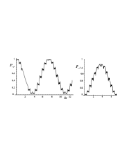
FIG. 1.: Time dependence of the populations $P_{\mu}$ for the state $\left|\mu\right\rangle=\left|-J\right\rangle$ and $\left|\mu\right\rangle=\left|-J+1\right\rangle.$ The parameters are taken as $\delta/\kappa=0.25$, $\varepsilon_{1}/\kappa=14$, $\omega/\kappa=3$, $N=2J=16$.

If one chooses the frequency $\omega$ such that the resonance condition (31) holds at certain integer $n_{0},$ the corresponding harmonic can be made dominant. Indeed, provided that $\left|U_{\mu}^{n}\right|\ll 1$ for $\mu=-J+1$, for all $n$, coupling to other states is weak, and we have an effective two-level system. This is possible provided that at resonance $\omega$ is large compared with $\kappa$, which in turn is large compared with the coupling parameter $\delta$. This is demonstrated in Fig. 1, where oscillations between the states $\left|-J\right\rangle$ and $\left|-J+1\right\rangle$ are displayed for the initial state (34). This means that a single atom out of $N$ atoms resonantly oscillates between the wells. Upon decreasing the coupling between the wells, the rate of off-resonant coupling is decreasing, so one approaches ideal Rabi oscillations between resonant levels. Weaker coupling implies a larger oscillation period. The two-level behavior can only occur for a system with a nonlinear term $\widehat{J}_{z}^{2}$, since for a linear system the various transitions are simultaneously in resonance [6] and [7].

In the case that the modulation frequency $\omega$ is of the same order as $\kappa$, resonances on the different transitions can coincide, and the initial state (34) can spread out over many number states. For example, in the simple case that $\omega=\kappa$, the resonance condition (31) shows that for each value of $\mu$, there is a harmonic $n=-(2\mu+1)$ that is resonant, and the population spreads out over all number states.

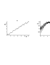
FIG. 2.: Time dependence of the fluctuation $\left\langle\widehat{J}_{z}\right\rangle^{2}$ of operator $\widehat{J}_{z}$ at resonance (a) $\omega=\kappa$ and out of resonance (b) $\omega=6\kappa.$ The other parameters are taken the same as in the previous figure.

The difference with the high-frequency case is demonstrated in Fig. 2, where we plot the fluctuations $\Delta J_{z}^{2}$ of $\widehat{J}_{z}$ as a function of time, for the initial condition (34), for $\omega=4\kappa$ (a) and $\omega=\kappa$ (b). In the first case, the fluctuations remain limited. In the second case, a resonance occurs on each transition, and $\Delta J_{z}^{2}$ continues to increase. Even for a very small coupling between wells, resonances designed in such a way can lead to enhancement in the tunneling rate. This is close to the experimental situation for the double-well trap presented in Ref. [4]. Again, this situation is specific for a system with a non-linear term $\widehat{J}_{z}^{2}$ in the Hamiltonian, since for a linear system various transitions have the same effective coupling. Since the coupling is proportional to $J_{n}\left(\varepsilon_{1}/\omega\right)$, a resonant transition can be turned off by setting the ratio $\varepsilon_{1}/\omega$ equal to a zero of the Bessel function.

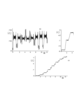
FIG. 3.: Time dependence of the expectation value of $\widehat{J}_{z}$ operator is plotted at resonance $\omega=\kappa$. The ratio $\varepsilon_{1}/\omega$ is chosen such that (a) $\varepsilon_{1}/\omega=24.26918$ ($J(_{13}\left(\varepsilon_{1}/\omega\right)=0$) , (b) $\varepsilon_{1}/\omega=23.2759$ ($J_{11}\left(\varepsilon_{1}/\omega\right)=0)$ (c) $\varepsilon_{1}/\omega=24.93493$ ($J_{7}\left(\varepsilon_{1}/\omega\right)=0$). The total number of particles is chosen $N=16$.

This can be used to restrict the evolution to a limited number of states, thereby locating a desired number of particles in one of the wells. We demonstrate this idea in Fig. 3. There we start from the same initial condition (34) and see that $11$ atoms out of $16$ are localized in the left well if one chooses the ratio $\varepsilon_{1}/\omega$ such that $J_{7}\left(\varepsilon_{1}/\omega\right)=0$ (Fig. 3a). Then, taking $J_{11}\left(\varepsilon_{1}/\omega\right)=0$, or $J_{15}\left(\varepsilon_{1}/\omega\right)=0$, one can localize $13$ or $16$ particles in one of the wells (Figs. 3b and 3c).

VI Generalization to an optical lattice

The discussion of the previous section for two wells with an energy difference can be generalized to the case of a multimode system, consisting of a chain of potential wells. As a model, we take a BEC in a tilted optical lattice [7]. As usual, we neglect the higher bands in the lattice, and we consider only a BEC trapped in the lowest energy band, that roughly speaking is composed of the ground states in all the wells [15]. If one takes the Wannier states $\left|l\right\rangle$ with $l=\ldots-2$, $-1$, $0$, $1$, $2$, $\ldots$as the basis of one-particle states, the Hamiltonian in second quantization is a direct generalization of Eq. (6) for two wells, and it takes the form

$$\widehat{H}_{BH}=-\frac{\hbar\delta}{2}\sum_{l}\left(\widehat{a}_{l+1}^{\dagger}\widehat{a}_{l}+\widehat{a}_{l}^{\dagger}\widehat{a}_{l+1}\right)+\frac{\hbar\kappa}{2}\sum_{l}\widehat{a}_{l}^{\dagger}\widehat{a}_{l}^{\dagger}\widehat{a}_{l}\widehat{a}_{l}+\hbar\varepsilon\left(t\right)\sum_{l}l\widehat{a}_{l}^{\dagger}\widehat{a}_{l},$$ (35)

where $\widehat{a}_{l\text{ }}\left(\widehat{a}_{l\text{ }}^{\dagger}\right)$ are bosonic annihilation (creation) operators in a single Wannier state, $\delta$ and $\kappa$ are the obvious multimode generalizations of two-mode definitions for the nearest neighbor coupling and interaction constant (1, 7), $\varepsilon$ is the energy difference in frequency units between neighboring Wannier states, which determines the uniform force. This Hamiltonian defines the so-called Bose-Hubbard model.

The time evolution in a lattice is governed by the time-dependent Schrödinger equation

$$i\hbar\frac{d\left|\Psi\left(t\right)\right\rangle}{dt}=\widehat{H}_{BH}\left|\Psi\left(t\right)\right\rangle.$$ (36)

The uniform force and the interatomic interaction can be eliminated by the substitution

$\displaystyle\left|\Psi_{BH}\left(t\right)\right\rangle=\widehat{T}_{BH}(t)\left|\Psi_{BH}^{{}^{\prime}}\left(t\right)\right\rangle,$

with

$\displaystyle\widehat{T}_{BH}(t)=\exp\left(-i\theta\left(t\right)\sum_{l}l\widehat{a}_{l}^{\dagger}\widehat{a}_{l}-\frac{i\kappa t}{2}\sum_{l}\widehat{a}_{l}^{\dagger}\widehat{a}_{l}^{\dagger}\widehat{a}_{l}\widehat{a}_{l}\right)$

and $\theta\left(t\right)=\int_{0}^{t}dt^{{}^{\prime}}\varepsilon\left(t^{{}^{\prime}}\right)$ is the area of pulse. The Schrödinger equation for the transformed state $\left|\Psi_{BH}^{{}^{\prime}}\left(t\right)\right\rangle$ follows by using the transformation properties of the annihilation operator

$\displaystyle\widehat{T}_{BH}^{\dagger}(t)\widehat{a}_{l}\widehat{T}_{BH}(t)=\widehat{a}_{l}\exp\left(-il\theta(t)-i\kappa t\left(\widehat{a}_{l}^{\dagger}\widehat{a}_{l}-1\right)\right)=\exp\left(-il\theta(t)-i\kappa t\widehat{a}_{l}^{\dagger}\widehat{a}_{l}\right)\widehat{a}_{l},$

which leads to the identity

$\displaystyle\widehat{T}_{BH}^{\dagger}(t)\widehat{a}_{l+1}^{\dagger}\widehat{a}_{l}\widehat{T}_{BH}(t)=\widehat{a}_{l+1}^{\dagger}\widehat{a}_{l}\exp\left[i\theta(t)+i\kappa t\left(\widehat{a}_{l+1}^{\dagger}\widehat{a}_{l+1}-\widehat{a}_{l}^{\dagger}\widehat{a}_{l}+1\right)\right].$

We obtain the evolution equation

$$i\hbar\frac{d\left|\Psi_{BH}^{\prime}\left(t\right)\right\rangle}{dt}=\widehat{H}_{BH}^{{}^{\prime}}\left|\Psi_{BH}^{\prime}\left(t\right)\right\rangle,$$ (37)

with the effective Hamiltonian

$$\widehat{H}_{BH}^{{}^{\prime}}=-\frac{\hbar\delta}{2}\sum_{l}\left(\widehat{a}_{l+1}^{\dagger}\widehat{a}_{l}\exp\left[i\theta(t)+i\kappa t\left(\widehat{a}_{l+1}^{\dagger}\widehat{a}_{l+1}-\widehat{a}_{l}^{\dagger}\widehat{a}_{l}+1\right)\right]+\text{H.c.}\right).$$ (38)

For the case of a periodically modulated uniform force, described by $\varepsilon\left(t\right)=\varepsilon_{1}\cos\omega t$, this Hamiltonian can be put in the form

$$\widehat{H}_{BH}^{{}^{\prime}}=-\frac{\hbar\delta}{2}\sum_{l}\sum_{n}J_{n}\left(\frac{\varepsilon_{1}}{\omega}\right)\left(\widehat{a}_{l+1}^{\dagger}\widehat{a}_{l}\exp\left[in\omega t+i\kappa t\left(\widehat{a}_{l+1}^{\dagger}\widehat{a}_{l+1}-\widehat{a}_{l}^{\dagger}\widehat{a}_{l}+1\right)\right]+\text{H.c.}\right).$$ (39)

This Hamiltonian couples collective number states $\left|\overrightarrow{N}\right\rangle=\left|\ldots,N_{-1},N_{0},N_{1},\ldots\right\rangle$ where two neighboring wells $l$ and $l+1$ have exchanged one particle. The coupling between states with $N_{l}=p$, $N_{l+1}=q$ and $N_{l}=p-1$, $N_{l+1}=q+1$ is resonant for a harmonic $n$ when

$$n\omega+\kappa\left(q-p+1\right)=0,$$ (40)

which is analogous to the resonance condition (31). At small tunneling rate we can exclude non-resonant coupling terms while assuming that their effective coupling rate is negligible. When the uniform force also contains a constant term, so that $\varepsilon(t)=\varepsilon_{0}+\varepsilon_{1}\cos\omega t$, we have to add a term $\varepsilon_{0}t$ to $\theta(t)$, and the resonance condition is modified into

$$n\omega+\varepsilon_{0}+\kappa\left(q-p+1\right)=0.$$ (41)

When $p-q=1$, this condition is independent of $\kappa$, and a resonant oscillation can occur between states with $N_{l}-N_{l+1}=\pm 1$.

Another interesting case is a Mott insulator state, with the same number of particles $N_{0}$ in each well. Such a state has been predicted in [15] and has been recently experimentally realized in ([16]), where one (two) atoms have been put in a single lattice site. So, $\left|\Psi\left(t=0\right)\right\rangle=\left|\ldots,N_{0},N_{0},N_{0},\ldots,\right\rangle.$ This state is directly coupled to the collective Fock state which arises if a boson escapes to a neighbouring well, so it has $N_{0}+1$ atoms in one lattice site, and $N_{0}-1$ in the neighboring one. Then the resonant condition is $n\omega+\varepsilon_{0}+\kappa=0$.

Just as in the case of two wells, resonances coincide when $\omega$ is of the same order as $\kappa$. When $\omega=\kappa$, there is always a harmonic that resonantly couples neighboring wells. In the absence of the constant term $\varepsilon_{0}$, the resonance condition takes the universal form $n+q-p+1=0$. So, if in the Mott insulator phase the number fluctuations are suppressed between wells, we obtain their increase at resonances.

VII Periodic modulation of coupling

In this Section we consider the effects of a periodic modulation of the coupling coefficient $\delta(t)$ between the wells. As a simple model, we assume that $\delta$ contains a harmonic component, so that

$$\delta\left(t\right)=\delta_{0}+\delta_{1}\cos\omega t.$$ (42)

In order that the even state $\left|g\right\rangle=(\left|1\right\rangle+\left|2\right\rangle)/\sqrt{2}$ is the ground state, we keep $\delta(t)$ positive at all times, and we choose $\delta_{1}$ to be smaller than $\delta_{0}$. Hence we assume that $\delta_{0}\geq\delta_{1}\geq 0$. Moreover, we take the energy of the two wells to be equal, so that $\varepsilon=0$. The Hamiltonian in the form of (11) with the coupling coefficient (42) can be easily implemented in practice. It describes a BEC in a two-well configuration with a periodically modulated barrier height. Precise calculations of the coupling coefficient are given in [5].

Since in the Hamiltonian (11) the term proportional to $\widehat{J}_{x}$ is periodically modulated, we expect that the basis of states $\left|\mu\right\rangle_{x}$, which are eigenstates of the operator $\widehat{J}_{x}$, is the natural basis to describe the evolution. Then it is convenient to describe the Hamiltonian in terms of the operators $\widehat{J}_{x}$ and $\widehat{J}_{x}^{\pm}$, which are defined in Eq. (19). By using the identities $\widehat{J}_{z}=-(\widehat{J}_{x}^{+}+\widehat{J}_{x}^{-})/2$ and $\widehat{J}_{x}^{+}\widehat{J}_{x}^{-}+\widehat{J}_{x}^{-}\widehat{J}_{x}^{+}=2[J(J+1)-\widehat{J}_{x}^{2}]$, we rewrite the $N$-particle Hamiltonian (11) in the form

$$\widehat{H}_{N}=-\hbar\delta\left(t\right)\widehat{J}_{x}+\frac{\hbar\kappa}{2}\left(J(J+1)-\widehat{J}_{x}^{2}\right)+{\displaystyle{\hbar\kappa\over 4}}\left(\widehat{J}_{x}^{+2}+\widehat{J}_{x}^{-2}\right).$$ (43)

This expression demonstrates that a state $\left|\mu\right\rangle_{x}$ is coupled only to its next nearest neighbors $\left|\mu\pm 2\right\rangle_{x}$. The coupling strength is measured by the matrix element

$$\Omega_{\mu}^{x}=\frac{\kappa}{4}\text{ }_{x}\left\langle\mu+2\right|\widehat{J}_{x}^{+2}\left|\mu\right\rangle_{x}=\frac{\kappa}{4}\sqrt{\left(J+\mu+1\right)\left(J+\mu+2\right)\left(J-\mu-1\right)\left(J-\mu\right)},$$ (44)

which depends on the interparticle interaction coefficient $\kappa$ and the particle number $N=2J$.

In order to get a closer insight to the role of periodic modulation and its resonances, we again eliminate the diagonal part of the Hamiltonian, now with respect to the basis of states $\left|\mu\right\rangle_{x}$. The time-dependent state is expressed

$$\left|\Psi\left(t\right)\right\rangle=\widehat{S}(t)\left|\Psi^{\prime\prime}\left(t\right)\right\rangle,$$ (45)

with

$$\widehat{S}(t)=\exp\left[i\eta\left(t\right)\widehat{J}_{x}-\frac{1}{2}i\kappa t\left(J(J+1)-\widehat{J}_{x}^{2}\right)\right],$$ (46)

and $\eta\left(t\right)=\int_{0}^{t}dt^{{}^{\prime}}\delta\left(t^{{}^{\prime}}\right)$ is the integrated coupling coefficient. In order to obtain the Schrödinger equation for the transformed state $\left|\Psi^{\prime\prime}\left(t\right)\right\rangle$, we need the transformation property of the off-diagonal operators $\widehat{J}_{x}^{+2}$ and $\widehat{J}_{x}^{-2}$. The transformed state $\left|\Psi^{\prime\prime}(t)\right\rangle$ obeys the Schrödinger equation with the effective Hamiltonian

$\displaystyle\widehat{H}^{\prime\prime}(t)={\displaystyle{\hbar\kappa\over 4}}\widehat{S}^{\dagger}(t)\left(\widehat{J}_{x}^{+2}+\widehat{J}_{x}^{-2}\right)\widehat{S}(t).$

In analogy to Eq. (29), we now apply the general transformation rule

$$g(\widehat{J}_{x})\widehat{J}_{x}^{+2}=\widehat{J}_{x}^{+2}g(\widehat{J}_{x}+2),$$ (47)

for an arbitrary analytical function $g$ of $\widehat{J}_{x}$. After making a Fourier expansion we obtain for $\widehat{H}^{\prime\prime}(t)$ the explicit expression

$$\widehat{H}^{\prime\prime}(t)=\frac{\hbar\kappa}{4}\sum_{n=-\infty}^{\infty\text{ }}J_{n}\left({\displaystyle{2\delta_{1}\over\omega}}\right)\left[\widehat{J}_{x}^{+\text{ }2}e^{-it\left(\delta_{0}+2\kappa\left(\widehat{J}_{x}+1\right)+n\omega\right)}+\text{H.c.}\right]$$ (48)

The form of the Hamiltonian $\widehat{H}^{\prime\prime}(t)$ resembles the Hamiltonian $\widehat{H}^{\prime}(t)$, as specified in Eq. (30). In the present case, the basis states are the states $\left|\mu\right\rangle_{x}$, which are now coupled by the square of the corresponding ladder operator $\widehat{J}_{x}^{\pm\text{ }2}$. As in (30), the coupling term is a series of harmonics with equidistant frequencies $n\omega$, with an amplitude proportional to the Bessel function of the corresponding order.

In the high-frequency limit, when the modulation frequency $\omega$ is large compared with the diagonal frequency splittings of the Hamiltonian (43), the effect of the static term proportional to $J_{0}(2\delta_{1}/\omega)$ in Eq. (48) will be dominant, and the Hamiltonian will be effectively constant. Just as in precious sections, the physical reason is that a rapidly modulated field, which has a negligible average pulse area, also has a negligible influence.

On the other hand, Eq. (48) immediately shows that the coupling between the state $\left|\mu\right\rangle_{x}$ and $\left|\mu+2\right\rangle_{x}$ of the $n$th harmonic is resonant when

$$n\omega+2\kappa(\mu+1)+\delta_{0}=0.$$ (49)

The other coupling terms are negligible when the coupling strength is small compared with the oscillation frequency, which leads to the weak-coupling criterion

$$\left|\frac{\Omega_{\mu}^{x}}{n\omega+2\kappa\left(\mu+1\right)+\delta_{0}}J_{n}\left({\displaystyle{2\delta_{1}\over\omega}}\right)\right|\ll 1.$$ (50)

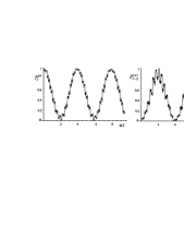
FIG. 4.: Time dependence of the populations $P_{\mu}^{\left(x\right)}$ of the state $\left|\mu\right\rangle_{x}$ with $\mu=J$ and $\mu=J-2$. The other parameters are taken as $\delta_{1}/\kappa=14$, $\delta_{0}/\kappa=16$, $\omega/\kappa=20$, $N=14$.

So, if the initial state $\left|\Psi\left(0\right)\right\rangle=$ $\left|J\right\rangle_{x}$ is resonantly coupled to $\left|J-2\right\rangle_{x}$, while further couplings of this alter state are negligible, we have an effective two-level system. This is demonstrated on the figure 4, where besides the resonant oscillations, one obtains non-resonant escape of population to the rest of manifold. Upon decreasing the coupling between the state $\left|\mu\right\rangle_{x}$, only the resonant states are involved and they exhibit clear Rabi oscillations. This shows how resonances lead to an escape of population from the initial state to the other states in the manifold of states $\left|\mu\right\rangle_{x}$. The similarity with the response to the periodic modulation in the form of a periodically modulated energy difference between the wells. Recall that the state $\left|J\right\rangle_{x}$ is the state in which all particles are in the even state $\left|g\right\rangle=(\left|1\right\rangle+\left|2\right\rangle)/\sqrt{2}$, which is the one-particle ground state. In the state $\left|J-2\right\rangle_{x}$, two particle have been transferred to the odd excited state.

VIII Conclusions

A BEC trapped in a two-well potential can be expected to be very sensitive to the frequency of any applied periodic perturbation. We test this idea by periodically modulating the asymmetry or the barrier height of such a configuration. Compared with the analogous situation of a single atom trapped in a light field with a periodic modulation, the many-particle nature of the BEC gives rise to some new effects. For both types of modulation, two-state resonances may be observed, where a single atom out of the BEC oscillates between the wells. It is also possible to enter a regime of parameters where more than two states are resonantly coupled, with more than one particle oscillating between the wells. Using such resonances, one can manipulate the average number of particles in the wells by varying the relevant parameters, such as the magnitude and the modulation frequency of the energy difference. This effect can be considered also as a means to resonantly enhance the tunnelling rate between wells. We generalize the basic ideas developed for two-wells to a multiwell system, such as a BEC in an optical lattice. Whereas the periodic modulation of the energy difference is related to coupling between number states in the two wells, the periodic modulation of the height of the barrier leads to coupling between number states in superposition states of the two wells with specific values of the relative phase.

REFERENCES

- [1] M. R. Andrews et al and W. Ketterle, Science 275, 637 (1997); D. S. Hall, M. R. Matthews, C. E. Wieman and E. A. Cornell Phys. Rev. Lett 81, 1543 (1998).
- [2] A. Polkovnikov, S. Sachdev and S. M. Girvin, Phys. Rev. A 66, 053607 (2002); J. R. Anglin and A. Vardi, Phys. Rev. A 64, 013605 (2001).
- [3] H. L. Haroutyunyan and G. Nienhuis Phys. Rev. A 67, (2003) 053611.
- [4] T. G. Tiecke, M. Kemmann, Ch. Buggle, I. Shvarchuck, W. von Klitzing and J. T. M. Walraven, J. Opt. B: Quantum Semiclass. Opt. 5, 119 (2003).
- [5] G. L. Salmond, C. A. Holmes and G. J. Milburn Phys. Rev. A. 65, 033623 (2002).
- [6] D.H. Dunlap and V.M. Kenkre, Phys. Rev. B 34, 3625 (1986).
- [7] H. L. Haroutyunyan and G. Nienhuis, Phys. Rev. A. 64, 033424 (2001).
- [8] G. S. Agarwal and W. Harshawardhan, Phys. Rev. A 50, R4465 (1994).
- [9] F. T. Arecchi and E. Courtens and R. Gilmore and H. Thomas Phys Rev A 6, 2211 (1972).
- [10] A. M. Perelomov, Generalized Coherent States and their applications (Springer, Berlin 1986).
- [11] Y. Castin and J. Dalibard, Phys. Rev. A 55, 4330 (1997).
- [12] F. A. M. de Oliveira, M. S. Kim and P. L. Knight, V. Bužek, Phys. Rev. A 41, 2645 (1990).
- [13] M. Greiner, O. Mandel, T.W. Hänsch and I. Bloch, Nature 419, 51 (2002).
- [14] M. Kitagawa and M. Ueda, Phys. Rev. A 47, 5138 (1993).
- [15] D. Jaksch, C. Bruder, J. I. Cirac, C. W. Gardiner, and P. Zoller, Phys. Rev. Lett. 81, 3108 (1998); A. R. Kolovsky Phys. Rev. Lett. 90, 213002 (2003); D. van Oosten, P. van der Straten, and H. T. C. Stoof, Phys. Rev. A 63, 053601 (2001); G. G. Batrouni, V. Rousseau, R. T. Scalettar, M. Rigol, A. Muramatsu, P. J. H. Denteneer, and M. Troyer, Phys. Rev. Lett. 89, 117203 (2002).
- [16] M. Greiner, O. Mandel, T. Esslinger, T. W. Hänsch and I. Bloch, Nature 415, 39 (2002).