Probabilities of failure for quantum error correction

Abstract

We investigate the performance of a quantum error-correcting code when pushed beyond its intended capacity to protect information against errors, presenting formulae for the probability of failure when the errors affect more qudits than that specified by the code’s minimum distance. Such formulae provide a means to rank different codes of the same minimum distance. We consider both error detection and error correction, treating explicit examples in the case of stabilizer codes constructed from qubits and encoding a single qubit.

I Introduction

Quantum error-correcting codes calderbank ; gottesman ; knill ; preskill ; nielsen ; grassl protect quantum information against noise. They play important roles in many areas of quantum information theory, but most critically, in the viability of a quantum computer. Quantum error correction negates a quantum state’s natural susceptibility to decohere, and thus provides the long-time coherence necessary to sustain quantum computation. Shor shor2 and Steane steane presented the first constructions of quantum error-correcting codes. These discoveries led to a formal connection between quantum codes and classical additive codes calderbank , and consequently, the characterization of a general class of quantum error-correcting codes commonly referred to as stabilizer codes gottesman .

The idea behind quantum error correction is to encode quantum states into qudits in such a way that a small number of errors affecting the individual qudits can be detected and corrected to perfectly restore the original encoded state. In this article we investigate the integrity of a quantum error-correcting code when under the influence of errors affecting more qudits than what the code was originally designed to handle. We derive general formulae to calculate the probabilities of successful error detection or correction, when the errors are depolarizing, and we are given either (i) the location of the errors, (ii) the number of errors, or, (iii) the probability that a single qudit is in error. Such formulae provide a means to compare codes of the same minimum distance. For the analysis of error detection we treat general quantum error-correcting codes constructed from qudits. This extends the results of Ashikhmin et al ashikhmin2 . We then specialize to stabilizer codes for the case of error correction, where the dimension of the constituent qudit subsystems is a prime power.

When the constituent subsystems are qubits, we give explicit results for a variety of stabilizer codes encoding a single qubit. We find that, for the depolarizing channel under error detection, as the number of qubits increases we are generally able to construct better codes even when the minimum distance remains constant. However this is not so for error correction. In this case the unique five-qubit quantum Hamming code outperforms all other codes of minimum distance three.

The article is organized as follows. In the next section we introduce quantum error-correcting codes, giving conditions for a code to have a specified minimum distance in terms of its weight enumerators. We then build on this treatment to analyze error detection in Sec. III, and error correction in Sec. IV, where stabilizer codes are also introduced. In Sec. V we characterize stabilizer codes constructed from qubits in terms of classical additive codes, giving many examples which we then investigate. Finally, in Sec. VI we review the main results of the article.

II Quantum error-correcting codes

The idea behind quantum error correction calderbank ; gottesman ; knill ; preskill ; nielsen ; grassl is to encode quantum states into qudits in such a way that a small number of errors affecting the individual qudits can be measured and corrected to perfectly restore the original encoded state. The encoding of a $K$-dimensional quantum state into $n$ qudits is simply a linear map from $\mathbb{C}^{K}$ to a subspace $\mathcal{Q}$ of $(\mathbb{C}^{D})^{\otimes n}$. The subspace itself is referred to as the code and is orientated in such a way that errors on the qudits move encoded states in a direction perpendicular to the code. We will refer to such codes as $((n,K))_{D}$ quantum error-correcting codes.

An error operator $E$ is a linear operator acting on $(\mathbb{C}^{D})^{\otimes n}$. The error is said to be detectable by the quantum code $\mathcal{Q}$ if

$$\langle\psi|E|\psi\rangle=\langle\phi|E|\phi\rangle$$ (1)

for all normalized $|\psi\rangle,|\phi\rangle\in\mathcal{Q}$. It is a general theorem of quantum error correction that a set of errors $\mathcal{E}$ can be corrected by a code $\mathcal{Q}$, if and only if for each $E_{1},E_{2}\in\mathcal{E}$, the error $E_{2}^{\dagger}E_{1}$ is detectable by $\mathcal{Q}$ knill .

Define the support of an error operator $E$, denoted by $\operatorname{supp}(E)$, as the subset of $\{1,\dots,n\}$ consisting of all indices labeling a qudit where $E$ acts nontrivially i.e. $E$ is not a scalar multiple of the identity on the qudit. The weight of $E$ is then the cardinality of $\operatorname{supp}(E)$, $\operatorname{wt}(E)\equiv|\operatorname{supp}(E)|$. A quantum code $\mathcal{Q}$ has a minimum distance of at least $d$ if and only if all errors of weight less than $d$ are detectable by $\mathcal{Q}$. A code with minimum distance $d$ allows the correction of arbitrary errors affecting $<d/2$ qudits. Such codes are denoted by the triple $((n,K,d))_{D}$. An $((n,K,d))_{D}$ code is called pure if $\langle\psi|E|\psi\rangle=D^{-n}\operatorname{tr}{E}$ for all $|\psi\rangle\in\mathcal{Q}$ whenever $\operatorname{wt}(E)<d$. The notion of pure is equivalent to nondegenerate for stabilizer codes calderbank ; gottesman . When considering self-dual codes ($K=1$), we adopt the convention that the notation $((n,1,d))_{D}$ refers only to pure codes since the condition on the minimum distance is otherwise trivial.

The remainder of this section is based on an article on quantum weight enumerators by Rains rains4 . We start with a lemma.

Lemma 1.

Let $\mathcal{Q}\leq\mathbb{C}^{N}$ with dimension $K$ and associated projector $P$. Furthermore denote by $\mathop{\operatorname{E}}_{\psi\in\mathcal{Q}}[\,\cdot\,]$ the unitarily invariant uniform average over all $|\psi\rangle\in\mathcal{Q}$. Then

$$\mathop{\operatorname{E}}_{\psi\in\mathcal{Q}}\left[|\psi\rangle\langle\psi|^{\otimes t}\right]=\frac{t!(K-1)!}{(t+K-1)!}\Pi_{\text{\rm sym}}^{t}$$ (2)

where $\Pi_{\text{\rm sym}}^{t}$ is the projector onto the totally symmetric subspace of $\mathcal{Q}^{\otimes t}$. In particular

$$\mathop{\operatorname{E}}_{\psi\in\mathcal{Q}}\left[|\psi\rangle\langle\psi|\right]=\frac{P}{K}\qquad\text{and}\qquad\mathop{\operatorname{E}}_{\psi\in\mathcal{Q}}\left[|\psi\rangle\langle\psi|\otimes|\psi\rangle\langle\psi|\right]=\frac{(P\otimes P)(1+T)}{K(K+1)}$$ (3)

where $T$ is the swap on $\mathbb{C}^{N}\!\!\otimes\mathbb{C}^{N}$ i.e. $T|\psi\rangle\otimes|\phi\rangle=|\phi\rangle\otimes|\psi\rangle$ for all $|\psi\rangle,|\phi\rangle\in\mathbb{C}^{N}$.

Proof.

Use Schur’s lemma. Eq. (2) is invariant under all unitaries $U^{\otimes t}$ which act irreducibly on the totally symmetric subspace $\Pi_{\text{sym}}^{t}\mathcal{Q}^{\otimes t}$. Also note that $\Pi_{\text{sym}}^{1}=P$ and $\Pi_{\text{sym}}^{2}=(P\otimes P)(1+T)/2$. $\Box$

Consider the variance in $\langle\psi|E|\psi\rangle$ over all states in the code

$$\mathop{\operatorname{Var}}_{\psi\in\mathcal{Q}}\left[\langle\psi|E|\psi\rangle\right]\equiv\mathop{\operatorname{E}}_{\psi\in\mathcal{Q}}\left[\big{|}\langle\psi|E|\psi\rangle-\mathop{\operatorname{E}}_{\phi\in\mathcal{Q}}\left[\langle\phi|E|\phi\rangle\right]\big{|}^{2}\right].$$ (4)

Using Lemma 1 we have the mean

$$\mathop{\operatorname{E}}_{\psi\in\mathcal{Q}}\left[\langle\psi|E|\psi\rangle\right]=\operatorname{tr}\left(E\mathop{\operatorname{E}}_{\psi\in\mathcal{Q}}\left[|\psi\rangle\langle\psi|\right]\right)=\frac{1}{K}\operatorname{tr}\left(EP\right)$$ (5)

and second moment

$$\mathop{\operatorname{E}}_{\psi\in\mathcal{Q}}\left[\langle\psi|E^{\dagger}|\psi\rangle\langle\psi|E|\psi\rangle\right] = \operatorname{tr}\left\{\left(E^{\dagger}\otimes E\right)\mathop{\operatorname{E}}_{\psi\in\mathcal{Q}}\left[|\psi\rangle\langle\psi|\otimes|\psi\rangle\langle\psi|\right]\right\}$$ (6)

$$= \frac{1}{K(K+1)}\operatorname{tr}\left[\left(E^{\dagger}\otimes E\right)\left(P\otimes P\right)(1+T)\right]$$ (7)

$$= \frac{1}{K(K+1)}\left[\operatorname{tr}\left(E^{\dagger}PEP\right)+\operatorname{tr}\left(E^{\dagger}P\right)\operatorname{tr}\left(EP\right)\right]$$ (8)

where we have used the fact that $\operatorname{tr}[(A\otimes B)T]=\operatorname{tr}(AB)$, and thus

$$\mathop{\operatorname{Var}}_{\psi\in\mathcal{Q}}\left[\langle\psi|E|\psi\rangle\right] = \mathop{\operatorname{E}}_{\psi\in\mathcal{Q}}\left[\langle\psi|E^{\dagger}|\psi\rangle\langle\psi|E|\psi\rangle\right]-\big{|}\mathop{\operatorname{E}}_{\psi\in\mathcal{Q}}\left[\langle\psi|E|\psi\rangle\right]\big{|}^{2}$$ (9)

$$= \frac{1}{K^{2}(K+1)}\left[K\operatorname{tr}\left(E^{\dagger}PEP\right)-\operatorname{tr}\left(E^{\dagger}P\right)\operatorname{tr}\left(EP\right)\right].$$ (10)

Now, by noting that an error $E$ is detectable if and only if the variance vanishes, we have the following equivalent definition of error detection.

Lemma 2.

Let $\mathcal{Q}$ be an $((n,K))_{D}$ quantum code with associated projector $P$. Then the error $E$ is detectable by $\mathcal{Q}$ iff $K\operatorname{tr}\left(E^{\dagger}PEP\right)=\operatorname{tr}\left(E^{\dagger}P\right)\operatorname{tr}\left(EP\right)$.

The multi-qudit displacement operators

$$\mathcal{D}(\bm{\mu},\bm{\nu})\equiv\mathcal{D}(\mu_{1}\dots\mu_{n},\nu_{1}\dots\nu_{n})\equiv D(\mu_{1},\nu_{1})\otimes\cdots\otimes D(\mu_{n},\nu_{n})\qquad 0\leq\mu_{k},\nu_{k}\leq D-1$$ (11)

where

$$D(\mu,\nu)\equiv e^{i\pi\mu\nu/D}X^{\mu}Z^{\nu},\qquad X|j\rangle\equiv|j+1\text{ mod }D\rangle,\qquad Z|j\rangle\equiv e^{2\pi ij/D}|j\rangle,$$ (12)

form an orthonormal basis for the set of all $n$-qudit operators:

$$A=D^{-n}\sum_{\bm{\mu},\bm{\nu}}\operatorname{tr}[\mathcal{D}(\bm{\mu},\bm{\nu})^{\dagger}A]\mathcal{D}(\bm{\mu},\bm{\nu}).$$ (13)

The weight of $\mathcal{D}(\bm{\mu},\bm{\nu})$ is simply the number of pairs $(\mu_{k},\nu_{k})$ different from $(0,0)$. For future reference we now note some properties of displacement operators:

$$D(\mu,\nu) = e^{i\pi\nu}D(\mu+D,\nu)\;=\;e^{i\pi\mu}D(\mu,\nu+D)$$ (14)

$$D(\mu,\nu)^{\dagger} = D(-\mu,-\nu)\;=\;e^{i\pi(\mu+\nu+D)}D(D-\mu,D-\nu)$$ (15)

$$D(\mu,\nu)^{D} = D(\mu D,\nu D)\;=\;e^{i\pi\mu\nu D}I$$ (16)

$$D(\mu,\nu)D(\alpha,\beta) = e^{2\pi i(\nu\alpha-\mu\beta)/D}D(\alpha,\beta)D(\mu,\nu)\;=\;e^{\pi i(\nu\alpha-\mu\beta)/D}D(\mu+\alpha,\nu+\beta)$$ (17)

$$\operatorname{tr}\left[D(\mu,\nu)^{{\dagger}}D(\alpha,\beta)\right] = D\delta_{\mu\alpha}\delta_{\nu\beta}.$$ (18)

Note that if the errors $E_{1}$ and $E_{2}$ are detectable, then any linear combination $c_{1}E_{1}+c_{2}E_{2}$ is also detectable. In particular, a linear space of errors $\left\{\sum c_{i}E_{i}|c_{i}\in\mathbb{C}\right\}$ is detectable if and only if all errors $E_{i}$ are detectable. By defining the enumerators

$$A_{S}^{\prime}(P) \equiv \frac{D^{|S|}}{K^{2}}\mathop{\operatorname{E}}_{\operatorname{supp}\mathcal{D}(\bm{\mu},\bm{\nu})\subseteq S}\left[\operatorname{tr}\left\{\mathcal{D}(\bm{\mu},\bm{\nu})^{\dagger}P\right\}\operatorname{tr}\left\{\mathcal{D}(\bm{\mu},\bm{\nu})P\right\}\right]$$ (19)

$$\equiv \frac{1}{D^{|S|}K^{2}}\sum_{\operatorname{supp}\mathcal{D}(\bm{\mu},\bm{\nu})\subseteq S}\operatorname{tr}\left[\mathcal{D}(\bm{\mu},\bm{\nu})^{\dagger}P\right]\operatorname{tr}\left[\mathcal{D}(\bm{\mu},\bm{\nu})P\right]$$ (20)

$$B_{S}^{\prime}(P) \equiv \frac{D^{|S|}}{K}\mathop{\operatorname{E}}_{\operatorname{supp}\mathcal{D}(\bm{\mu},\bm{\nu})\subseteq S}\left[\operatorname{tr}\left\{\mathcal{D}(\bm{\mu},\bm{\nu})^{\dagger}P\mathcal{D}(\bm{\mu},\bm{\nu})P\right\}\right]$$ (21)

$$\equiv \frac{1}{D^{|S|}K}\sum_{\operatorname{supp}\mathcal{D}(\bm{\mu},\bm{\nu})\subseteq S}\operatorname{tr}\left[\mathcal{D}(\bm{\mu},\bm{\nu})^{\dagger}P\mathcal{D}(\bm{\mu},\bm{\nu})P\right]$$ (22)

and noting that $D^{|S|}\left[B_{S}^{\prime}(P)-A_{S}^{\prime}(P)\right]/(K+1)$ is the sum over all positive quantities $\mathop{\operatorname{Var}}_{\psi\in\mathcal{Q}}\left[\langle\psi|\mathcal{D}(\bm{\mu},\bm{\nu})|\psi\rangle\right]$ with $\operatorname{supp}\mathcal{D}(\bm{\mu},\bm{\nu})\subseteq S$, we have the following lemma.

Lemma 3.

Let $\mathcal{Q}$ be an $((n,K))_{D}$ quantum code with associated projector $P$. Then all errors $E$ with $\operatorname{supp}E\subseteq S$ are detectable by $\mathcal{Q}$ iff $B_{S}^{\prime}(P)=A_{S}^{\prime}(P)$.

With the help of Eq. (17) we find that

$$\mathop{\operatorname{E}}_{\bm{\mu},\bm{\nu}}\left[\mathcal{D}(\bm{\mu},\bm{\nu})^{\dagger}A\mathcal{D}(\bm{\mu},\bm{\nu})\right] \equiv D^{-2n}\sum_{\bm{\mu},\bm{\nu}}\mathcal{D}(\bm{\mu},\bm{\nu})^{\dagger}A\mathcal{D}(\bm{\mu},\bm{\nu})$$ (23)

$$= D^{-3n}\sum_{\bm{\mu},\bm{\nu},\bm{\alpha},\bm{\beta}}\operatorname{tr}[\mathcal{D}(\bm{\alpha},\bm{\beta})^{\dagger}A]\mathcal{D}(\bm{\mu},\bm{\nu})^{\dagger}\mathcal{D}(\bm{\alpha},\bm{\beta})\mathcal{D}(\bm{\mu},\bm{\nu})$$ (24)

$$= D^{-3n}\sum_{\bm{\mu},\bm{\nu},\bm{\alpha},\bm{\beta}}\operatorname{tr}[\mathcal{D}(\bm{\alpha},\bm{\beta})^{\dagger}A]e^{2\pi i(\bm{\mu}\cdot\bm{\beta}-\bm{\alpha}\cdot\bm{\nu})/D}\mathcal{D}(\bm{\alpha},\bm{\beta})$$ (25)

$$= D^{-n}\sum_{\bm{\alpha},\bm{\beta}}\operatorname{tr}[\mathcal{D}(\bm{\alpha},\bm{\beta})^{\dagger}A]\delta_{\bm{\alpha}\bm{0}}\delta_{\bm{\beta}\bm{0}}\mathcal{D}(\bm{\alpha},\bm{\beta})$$ (26)

$$= D^{-n}\operatorname{tr}(A)I.$$ (27)

The following lemma now applies to the operators $\mathcal{D}(\bm{\mu},\bm{\nu})$.

Lemma 4.

Let $\mathop{\operatorname{E}}_{\Upsilon}[\,\cdot\,]$ denote the expectation (average), given some probability measure $d\mu(\Upsilon)$, over a set of linear operators $\{\Upsilon\}\subset\text{\rm End}(\mathbb{C}^{N})$. Then the following three statements are equivalent.

1. $\mathop{\operatorname{E}}_{\Upsilon}\left[\operatorname{tr}(\Upsilon^{\dagger}A)\Upsilon\right]=A/N$ for all linear operators $A$,

2. $\mathop{\operatorname{E}}_{\Upsilon}\left[\Upsilon^{\dagger}A\Upsilon\right]=\operatorname{tr}(A)I/N$ for all linear operators $A$,

3. $\mathop{\operatorname{E}}_{\Upsilon}\left[\Upsilon^{\dagger}\otimes\Upsilon\right]=T/N$, where $T$ is the swap.

Proof.

Since only 2 $\Leftrightarrow$ 3 is needed for the current article we will leave the remaining parts of the proof as an exercise for the reader.

Assuming 2 and letting $|j\rangle$ be a basis for $\mathbb{C}^{N}$, we have

$$\langle j|\otimes\langle k|\left({\textstyle\mathop{\operatorname{E}}_{\Upsilon}}\left[\Upsilon^{\dagger}\otimes\Upsilon\right]\right)|l\rangle\otimes|m\rangle=\langle j|{\textstyle\mathop{\operatorname{E}}_{\Upsilon}}\left[\Upsilon^{\dagger}|l\rangle\langle k|\Upsilon\right]|m\rangle=\delta_{kl}\delta_{jm}/N$$ (28)

and thus 2 $\Rightarrow$ 3. Assuming 3,

$$\langle l|{\textstyle\mathop{\operatorname{E}}_{\Upsilon}}\left[\Upsilon^{\dagger}A\Upsilon\right]|m\rangle = \sum_{j,k}{\textstyle\mathop{\operatorname{E}}_{\Upsilon}}\left[\langle l|\Upsilon^{\dagger}|j\rangle\langle j|A|k\rangle\langle k|\Upsilon|m\rangle\right]$$ (29)

$$= \sum_{j,k}\langle l|\otimes\langle k|\left({\textstyle\mathop{\operatorname{E}}_{\Upsilon}}\left[\Upsilon^{\dagger}\otimes\Upsilon\right]\right)|j\rangle\otimes|m\rangle\langle j|A|k\rangle$$ (30)

$$= \sum_{j,k}\delta_{jk}\delta_{ml}\langle j|A|k\rangle/N=\operatorname{tr}(A)\delta_{lm}/N$$ (31)

and thus 3 $\Rightarrow$ 2. $\Box$

With Lemma 4 in hand we find that

$$\mathop{\operatorname{E}}_{\operatorname{supp}\mathcal{D}(\bm{\mu},\bm{\nu})\subseteq S}\left[\operatorname{tr}\left\{\mathcal{D}(\bm{\mu},\bm{\nu})^{\dagger}P\right\}\operatorname{tr}\left\{\mathcal{D}(\bm{\mu},\bm{\nu})P\right\}\right] = \operatorname{tr}\left\{\mathop{\operatorname{E}}_{\operatorname{supp}\mathcal{D}(\bm{\mu},\bm{\nu})\subseteq S}\left[\mathcal{D}(\bm{\mu},\bm{\nu})^{\dagger}\otimes\mathcal{D}(\bm{\mu},\bm{\nu})\right](P\otimes P)\right\}$$ (32)

$$= D^{-|S|}\operatorname{tr}\left[T_{S}(P\otimes P)\right]$$ (33)

$$= D^{-|S|}\operatorname{tr}_{S}\left[(\operatorname{tr}_{S^{\prime}}P)^{2}\right]$$ (34)

where $T_{S}$ acts on $(\mathbb{C}^{D})^{\otimes n}\otimes(\mathbb{C}^{D})^{\otimes n}$ by swapping all qudits with indices in $S$, and

$$\mathop{\operatorname{E}}_{\operatorname{supp}\mathcal{D}(\bm{\mu},\bm{\nu})\subseteq S}\left[\operatorname{tr}\left\{\mathcal{D}(\bm{\mu},\bm{\nu})^{\dagger}P\mathcal{D}(\bm{\mu},\bm{\nu})P\right\}\right] = D^{-|S|}\operatorname{tr}\left[(\operatorname{tr}_{S}P)P\right]$$ (35)

$$= D^{-|S|}\operatorname{tr}_{S^{\prime}}\left[(\operatorname{tr}_{S}P)^{2}\right].$$ (36)

Consequently, our previously cumbersome definition of the weight enumerators (19-22) may be simplified to

$$A_{S}^{\prime}(P) = \frac{1}{K^{2}}\operatorname{tr}_{S}\left[(\operatorname{tr}_{S^{\prime}}P)^{2}\right]$$ (37)

$$B_{S}^{\prime}(P) = \frac{1}{K}\operatorname{tr}_{S^{\prime}}\left[(\operatorname{tr}_{S}P)^{2}\right].$$ (38)

It is easily verified that the normalization condition $A_{\emptyset}^{\prime}(P)=B_{\emptyset}^{\prime}(P)=1$ is satisfied, for self-dual codes $B_{S}^{\prime}(P)=A_{S}^{\prime}(P)$ for all $S\subseteq\{1,\dots,n\}$, and in general,

$$B_{S}^{\prime}(P)\geq A_{S}^{\prime}(P)>0$$ (39)

for all $S\subseteq\{1,\dots,n\}$. Also note that the above simplification (37,38) gives the relation

$$B_{S}^{\prime}(P)=KA_{S^{\prime}}^{\prime}(P).$$ (40)

Note from Eq. (20) that $D^{|T|}A_{T}^{\prime}(P)\leq D^{|S|}A_{S}^{\prime}(P)$ whenever $T\subseteq S$. We obtain a similar inequality from Eq. (22), and with the above relation (40), one may deduce that

$$D^{|T|-|S|}A_{T}^{\prime}(P)\leq\! A_{S}^{\prime}(P) \!\leq D^{|S|-|T|}A_{T}^{\prime}(P)$$ (41)

$$D^{|T|-|S|}B_{T}^{\prime}(P)\leq\! B_{S}^{\prime}(P) \!\leq D^{|S|-|T|}B_{T}^{\prime}(P)$$ (42)

whenever $T\subseteq S$. By diagonalizing $P=\sum_{k=1}^{K}|k\rangle\langle k|$, and using the Cauchy-Schwarz inequality, $|\operatorname{tr}AB^{\dagger}|^{2}\leq\operatorname{tr}AA^{\dagger}\operatorname{tr}BB^{\dagger}$, we find that $\operatorname{tr}_{S}\left[(\operatorname{tr}_{S^{\prime}}P)^{2}\right]=\sum_{j,k=1}^{K}\operatorname{tr}_{S}(\rho_{j}\rho_{k})\leq\sum_{j,k=1}^{K}\sqrt{\operatorname{tr}_{S}({\rho_{j}}^{2})\operatorname{tr}_{S}({\rho_{k}}^{2})}\leq K^{2}$ since $\operatorname{tr}_{S}({\rho_{k}}^{2})\leq 1$ where $\rho_{k}\equiv\operatorname{tr}_{S^{\prime}}|k\rangle\langle k|$. Now using this inequality on Eq.’s (37) and (38), and with $T=\emptyset$ in inequalities (41) and (42) we obtain various bounds for the weight enumerators. These reduce to

$$\max\left\{D^{-|S|},D^{|S|-n}/K\right\}\leq\! A_{S}^{\prime}(P) \!\leq\min\left\{1,D^{n-|S|}/K\right\}$$ (43)

$$\max\left\{D^{-|S|},KD^{|S|-n}\right\}\leq\! B_{S}^{\prime}(P) \!\leq\min\left\{D^{|S|},K\right\}.$$ (44)

Finally we remark that the weight enumerators are unchanged if we replace the operators $\mathcal{D}(\bm{\mu},\bm{\nu})$ used in the expectations (19) and (21) by any type of random depolarizing error (Definition 7). In particular we could choose random unitaries under the Haar measure as was done in their original definition rains4 .

We now define the Rains enumerators rains4

$$A_{m}^{\prime}(P) \equiv \sum_{|S|=m}A_{S}^{\prime}(P)=\frac{1}{K^{2}}\sum_{|S|=m}\operatorname{tr}_{S}\left[(\operatorname{tr}_{S^{\prime}}P)^{2}\right]$$ (45)

$$B_{m}^{\prime}(P) \equiv \sum_{|S|=m}B_{S}^{\prime}(P)=\frac{1}{K}\sum_{|S|=m}\operatorname{tr}_{S^{\prime}}\left[(\operatorname{tr}_{S}P)^{2}\right]$$ (46)

where $m=0,\dots,n$. These satisfy the normalization condition $A_{0}^{\prime}(P)=B_{0}^{\prime}(P)=1$, for self-dual codes $B_{m}^{\prime}(P)=A_{m}^{\prime}(P)$ for all $0\leq m\leq n$, and in general,

$$B_{m}^{\prime}(P)\geq A_{m}^{\prime}(P)>0$$ (47)

for all $0\leq m\leq n$. Again we have the relation

$$B_{m}^{\prime}(P)=KA_{n-m}^{\prime}(P)$$ (48)

and the inequalities

$$D^{l-m}A_{l}^{\prime}(P)\leq\! A_{m}^{\prime}(P) \!\leq D^{m-l}A_{l}^{\prime}(P)$$ (49)

$$D^{l-m}B_{l}^{\prime}(P)\leq\! B_{m}^{\prime}(P) \!\leq D^{m-l}B_{l}^{\prime}(P)$$ (50)

whenever $l\leq m$, and

$$\max\left\{D^{-m},D^{m-n}/K\right\}\leq\! \displaystyle\frac{m!(n-m)!}{n!}A_{m}^{\prime}(P) \!\leq\min\left\{1,D^{n-m}/K\right\}$$ (51)

$$\max\left\{D^{-m},KD^{m-n}\right\}\leq\! \displaystyle\frac{m!(n-m)!}{n!}B_{m}^{\prime}(P) \!\leq\min\left\{D^{m},K\right\}.$$ (52)

Finally, by noticing that $B_{m}^{\prime}(P)-A_{m}^{\prime}(P)=\sum_{|S|=m}B_{S}^{\prime}(P)-A_{S}^{\prime}(P)=0$ if and only if each term in the sum is zero, as a simple consequence of Lemma 3, we have the following theorem rains4 .

Theorem 5.

Let $\mathcal{Q}$ be an $((n,K))_{D}$ quantum code with associated projector $P$. Then $\mathcal{Q}$ has minimum distance of at least $d$ iff $B_{d-1}^{\prime}(P)=A_{d-1}^{\prime}(P)$.

Alternatively, one may define the Shor-Laflamme enumerators shor

$$A_{m}(P) \equiv \frac{1}{K^{2}}\sum_{\operatorname{wt}\mathcal{D}(\bm{\mu},\bm{\nu})=m}\operatorname{tr}[\mathcal{D}(\bm{\mu},\bm{\nu})^{\dagger}P]\operatorname{tr}[\mathcal{D}(\bm{\mu},\bm{\nu})P]$$ (53)

$$B_{m}(P) \equiv \frac{1}{K}\sum_{\operatorname{wt}\mathcal{D}(\bm{\mu},\bm{\nu})=m}\operatorname{tr}[\mathcal{D}(\bm{\mu},\bm{\nu})^{\dagger}P\mathcal{D}(\bm{\mu},\bm{\nu})P]$$ (54)

where $m=0,\dots,n$, which [from Eq.’s (20) and (22)] may be related to the Rains enumerators

$$A_{m}^{\prime}(P) = D^{-m}\sum_{i=0}^{m}\frac{(n-i)!}{(m-i)!(n-m)!}A_{i}(P)$$ (55)

$$B_{m}^{\prime}(P) = D^{-m}\sum_{i=0}^{m}\frac{(n-i)!}{(m-i)!(n-m)!}B_{i}(P)$$ (56)

and satisfy the normalization condition $A_{0}(P)=B_{0}(P)=1$, for self-dual codes $B_{i}(P)=A_{i}(P)$ for all $0\leq i\leq n$, and in general $B_{i}(P)\geq A_{i}(P)\geq 0$ for $0\leq i\leq n$. The above relations [Eq.’s (48), (55) and (56)] may be used to derive quantum versions of the MacWilliams identities, and thus, bounds on the parameters of a quantum code shor ; rains4 . Such bounds are the principle reason for defining quantum weight enumerators. We will show how weight enumerators also provide a means to quantify the performance of a code. For the Shor-Laflamme enumerators we have the following alternative to Theorem 5 shor .

Theorem 6.

Let $\mathcal{Q}$ be an $((n,K))_{D}$ quantum code with associated projector $P$. Then $\mathcal{Q}$ has minimum distance of at least $d$ iff $B_{i}(P)=A_{i}(P)$ for all $0<i<d$.

We conclude this section by remarking that an $((n,K,d))_{D}$ code is pure if and only if $B_{i}(P)=A_{i}(P)=0$ for all $0<i<d$ rains4 .

III Error detection

Consider an $((n,K))_{D}$ quantum code $\mathcal{Q}$ with $K>1$ and associated projector $P$. Given two orthonormal encoded states $|\phi\rangle,|\psi\rangle\in\mathcal{Q}$ ($\langle\phi|\psi\rangle=0$) we know that whenever an error $E$ is detectable

$$\langle\psi|E|\psi\rangle=\langle\phi|E|\phi\rangle=\left(\frac{\langle\phi|+\langle\psi|}{\sqrt{2}}\right)E\left(\frac{|\phi\rangle+|\psi\rangle}{\sqrt{2}}\right)=\left(\frac{\langle\phi|-i\langle\psi|}{\sqrt{2}}\right)E\left(\frac{|\phi\rangle+i|\psi\rangle}{\sqrt{2}}\right)=C(E)$$ (57)

where $C(E)$ is a constant depending only on $E$. From Eq. (57) one may easily deduce that $\langle\phi|E|\psi\rangle=0$, and thus

$$PE|\psi\rangle=\left(P-|\psi\rangle\langle\psi|+|\psi\rangle\langle\psi|\right)E|\psi\rangle=C(E)|\psi\rangle$$ (58)

since the projector $P-|\psi\rangle\langle\psi|$ is orthogonal to $|\psi\rangle$. Consequently, the projective measurement $\{P,1-P\}$, which tests whether or not our corrupted state $E|\psi\rangle$ is in the code, will either reveal an error or project $E|\psi\rangle$ back onto the original uncorrupted state $|\psi\rangle$. Remarkably, in the latter case the state is in fact corrected through measurement. In a scheme where a corrupted state is simply discarded once an error is detected, we can estimate the rate of transmission (i.e. the probability that a state is accepted) with the following theorem. We first, however, define what we mean by a random depolarizing error.

Definition 7.

A random depolarizing error $\Upsilon$ is a linear operator chosen randomly from a set $\{\Upsilon\}\subset\text{\rm End}(\mathbb{C}^{N})$ with probability measure $d\mu(\Upsilon)$, and the property that $\mathop{\operatorname{E}}_{\Upsilon}\left[\Upsilon^{\dagger}A\Upsilon\right]=\operatorname{tr}(A)I/N$ for all linear operators $A\in\text{\rm End}(\mathbb{C}^{N})$.

Note that if a set of random depolarizing errors $\{\Upsilon\}$ are to be considered as probabilistic quantum mechanical operations on a state $\rho$, then we must have the state $\Upsilon\rho\Upsilon^{\dagger}/\operatorname{tr}\left(\Upsilon^{\dagger}\Upsilon\rho\right)$ occurring with probability $\operatorname{tr}\left(\Upsilon^{\dagger}\Upsilon\rho\right)d\mu(\Upsilon)$. Also note that by our definition, Lemma 4 immediately applies to random depolarizing errors. We will call $\Upsilon_{S}$ a random depolarizing error acting on qudits $S$ when $\Upsilon_{S}$ acts nontrivially only on qudits with indices in $S\subseteq\{1,\dots,n\}$ of the multi-qudit state $|\psi\rangle\in(\mathbb{C}^{D})^{\otimes n}$. In this case $\mathop{\operatorname{E}}_{\Upsilon_{\!S}}\left[{\Upsilon_{S}}^{\dagger}A\Upsilon_{S}\right]=D^{-|S|}I_{S}\otimes\operatorname{tr}_{S}(A)$ for all linear operators $A\in\text{\rm End}\left((\mathbb{C}^{D})^{\otimes n}\right)$, where $I_{S}$ is the identity on qudits $S$. Some simple examples are listed below.

Example 1.

Let $\Upsilon_{S}$ be randomly chosen (with uniform probability $\mu(\Upsilon_{S})=D^{-2|S|}$) from the set $\{\mathcal{D}(\bm{\mu},\bm{\nu})|0\leq\mu_{k},\nu_{k}\leq D-1,\operatorname{supp}\mathcal{D}(\bm{\mu},\bm{\nu})\subseteq S\}$ of all displacement errors with support on a subset of $S$. Then $\Upsilon_{S}$ is a random depolarizing error acting on qudits $S$. This was shown in the previous section [Eq. (27)].

Example 2.

Let $\Upsilon_{S}$ be a unitary operator $U\in\text{U}\left(D^{|S|}\right)$ chosen randomly according to the Haar measure and with $\operatorname{supp}U=S$. From Schur’s lemma we have $\mathop{\operatorname{E}}_{\operatorname{supp}U\subseteq S}\left[U^{\dagger}AU\right]=D^{-|S|}I_{S}\otimes\operatorname{tr}_{S}(A)$ and thus $\Upsilon_{S}$ is a random depolarizing error acting on qudits $S$.

Example 3.

Let $\Upsilon_{S}$ be a local operator $\Upsilon_{S}=\bigotimes_{i\in S}\Upsilon_{i}$ with $\operatorname{supp}\Upsilon_{S}=S$, where each $\Upsilon_{i}$ is a random depolarizing error acting on qudit $i\in S$. Then

$${\textstyle\mathop{\operatorname{E}}_{\Upsilon_{\!S}}}\left[{\Upsilon_{S}}^{\dagger}\otimes\Upsilon_{S}\right]=\prod_{i\in S}{\textstyle\mathop{\operatorname{E}}_{\Upsilon_{\!i}}}\left[{\Upsilon_{i}}^{\dagger}\otimes\Upsilon_{i}\right]=\prod_{i\in S}\left(T_{i}/D\right)=D^{-|S|}T_{S}$$ (59)

and by Lemma 4, $\Upsilon_{S}$ is a random depolarizing error acting on qudits $S$.

The depolarizing channel on a single qudit $\rho$ is defined by the operation

$$\rho\rightarrow pI/D+(1-p)\rho$$ (60)

where $0\leq p\leq 1$ is the probability that the channel depolarizes the qudit. Note that, given a multi-qudit state $\rho$, we have

$${\textstyle\mathop{\operatorname{E}}_{\Upsilon_{\!i}}}\left[{\Upsilon_{i}}^{\dagger}\rho\Upsilon_{i}\right]=I_{i}/D\otimes\operatorname{tr}_{i}(\rho)$$ (61)

for arbitrary random depolarizing errors $\Upsilon_{i}$ acting on qudit $i$. Consequently, an error model of $n$ depolarizing channels corrupting each individual qudit independently is equivalent to an error process on $\rho$ where each local depolarizing error $\Upsilon_{S}\equiv\bigotimes_{i\in S}\Upsilon_{i}$ ($S\subseteq\{1,\dots,n\}$) occurs with probability $p^{|S|}\left(1-p\right)^{n-|S|}\prod_{i\in S}d\mu(\Upsilon_{i})$.

We now define the transmission rate to be the probability that no error is detected when an encoded state is corrupted by a random depolarizing error $\Upsilon$. Three different scenarios of a priori knowledge will be considered. We assume that either (i) the location of the corrupted qudits, $S=\operatorname{supp}\Upsilon$, is known, (ii) the number of corrupted qudits, $m=\operatorname{wt}\Upsilon$, is known, or (iii) the error is localized, $\Upsilon=\bigotimes_{i\in S}\Upsilon_{i}$, occurring with probability $p^{|S|}\left(1-p\right)^{n-|S|}\prod_{i\in S}d\mu(\Upsilon_{i})$ as in the aforementioned depolarizing channel, and the probability that a single qudit is corrupted, $p$, is known. Note that in all three cases the error detection procedure remains the same: a projection onto the code space. The probability of successful error detection, however, will depend on our a priori information about the error.

Definition 8.

Let $\mathcal{Q}$ be an $((n,K))_{D}$ quantum code with associated projector $P$, and let $\Upsilon_{S}$ be a random depolarizing error acting on qudits $S\subseteq\{1,\dots,n\}$ of an encoded pure state $|\psi\rangle\in\mathcal{Q}$, where the state is chosen randomly. Then the transmission rate on qudits $S$ under error detection, $\mathcal{T}^{\scriptscriptstyle d}_{S}(P)$, is defined as the probability that no error is detected in the corrupted state $|\psi^{\prime}\rangle=\Upsilon_{S}|\psi\rangle/\sqrt{\langle\psi|{\Upsilon_{S}}^{\dagger}\Upsilon_{S}|\psi\rangle}$, which occurs with probability $\langle\psi|{\Upsilon_{S}}^{\dagger}\Upsilon_{S}|\psi\rangle d\mu(\Upsilon_{S})$. That is

$$\mathcal{T}^{\scriptscriptstyle d}_{S}(P)\equiv{\textstyle\mathop{\operatorname{E}}_{\Upsilon_{\!S}}}\left[\mathop{\operatorname{E}}_{\psi\in\mathcal{Q}}\left[\langle\psi^{\prime}|P|\psi^{\prime}\rangle\langle\psi|{\Upsilon_{S}}^{\dagger}\Upsilon_{S}|\psi\rangle\right]\right]={\textstyle\mathop{\operatorname{E}}_{\Upsilon_{\!S}}}\left[\mathop{\operatorname{E}}_{\psi\in\mathcal{Q}}\left[\langle\psi|{\Upsilon_{S}}^{\dagger}P\Upsilon_{S}|\psi\rangle\right]\right].$$ (62)

If instead the errors act on $0\leq m\leq n$ unknown qudits, the transmission rate on $m$ qudits under error detection is

$$\mathcal{T}^{\scriptscriptstyle d}_{m}(P)\equiv\frac{m!(n-m)!}{n!}\sum_{|S|=m}\mathcal{T}^{\scriptscriptstyle d}_{S}(P)$$ (63)

which is again the probability that no error is detected. Finally, the transmission rate for the depolarizing channel under error detection is

$$\mathcal{T}^{\scriptscriptstyle d}_{p}(P)\equiv\sum_{m=0}^{n}p^{m}(1-p)^{n-m}\frac{n!}{m!(n-m)!}\mathcal{T}^{\scriptscriptstyle d}_{m}(P).$$ (64)

Now, by Lemma 1 and the definition of a random depolarizing error, we have

$${\textstyle\mathop{\operatorname{E}}_{\Upsilon_{\!S}}}\left[\mathop{\operatorname{E}}_{\psi\in\mathcal{Q}}\left[\langle\psi|{\Upsilon_{S}}^{\dagger}P\Upsilon_{S}|\psi\rangle\right]\right] = \frac{1}{K}{\textstyle\mathop{\operatorname{E}}_{\Upsilon_{\!S}}}\left[\operatorname{tr}\left({\Upsilon_{S}}^{\dagger}P\Upsilon_{S}P\right)\right]$$ (65)

$$= \frac{1}{D^{|S|}K}\operatorname{tr}\left[\left(\operatorname{tr}_{S}P\right)P\right]$$ (66)

$$= \frac{1}{D^{|S|}K}\operatorname{tr}_{S^{\prime}}\big{[}(\operatorname{tr}_{S}P)^{2}\big{]}\;,$$ (67)

and the following straightforward theorem.

Theorem 9.

Let $\mathcal{Q}$ be an $((n,K))_{D}$ quantum code with associated projector $P$. Then

$$\mathcal{T}^{\scriptscriptstyle d}_{S}(P) = D^{-|S|}B_{S}^{\prime}(P),$$ (68)

$$\mathcal{T}^{\scriptscriptstyle d}_{m}(P) = \frac{m!(n-m)!}{n!D^{m}}B_{m}^{\prime}(P),$$ (69)

and

$$\mathcal{T}^{\scriptscriptstyle d}_{p}(P)=\sum_{m=0}^{n}p^{m}(1-p)^{n-m}D^{-m}B_{m}^{\prime}(P).$$ (70)

Note that, given $D^{-|T|}B_{T}^{\prime}(P)\geq D^{-|S|}B_{S}^{\prime}(P)$ whenever $T\subseteq S$ [Eq. (42)], we must have

$$\mathcal{T}^{\scriptscriptstyle d}_{\emptyset}=1\geq\mathcal{T}^{\scriptscriptstyle d}_{T}(P)\geq\mathcal{T}^{\scriptscriptstyle d}_{S}(P)\geq\frac{K}{D^{n}}=\mathcal{T}^{\scriptscriptstyle d}_{\{1,\dots,n\}}$$ (71)

whenever $T\subseteq S$, and similarly

$$\mathcal{T}^{\scriptscriptstyle d}_{0}=1\geq\mathcal{T}^{\scriptscriptstyle d}_{l}(P)\geq\mathcal{T}^{\scriptscriptstyle d}_{m}(P)\geq\frac{K}{D^{n}}=\mathcal{T}^{\scriptscriptstyle d}_{n}$$ (72)

whenever $l\leq m$. Further bounds follow from Eq.’s (44) and (52).

The appropriate measure of success for quantum error detection is the average fidelity of all transmitted states. Again, we consider the three different cases of a priori information about the error.

Definition 10.

Let $\mathcal{Q}$ be an $((n,K))_{D}$ quantum code with associated projector $P$, and let $\Upsilon_{S}$ be a random depolarizing error acting on qudits $S\subseteq\{1,\dots,n\}$ of an encoded pure state $|\psi\rangle\in\mathcal{Q}$, where the state is chosen randomly. Then the transmission fidelity on qudits $S$ under error detection, $\mathcal{F}^{\scriptscriptstyle d}_{S}(P)$, is defined as the average fidelity of all transmitted states, given corrupted input states of the form $|\psi^{\prime}\rangle=\Upsilon_{S}|\psi\rangle/\sqrt{\langle\psi|{\Upsilon_{S}}^{\dagger}\Upsilon_{S}|\psi\rangle}$, which occur with probability $\langle\psi|{\Upsilon_{S}}^{\dagger}\Upsilon_{S}|\psi\rangle d\mu(\Upsilon_{S})$. That is

$$\mathcal{F}^{\scriptscriptstyle d}_{S}(P)\equiv\frac{{\textstyle\mathop{\operatorname{E}}_{\Upsilon_{\!S}}}\left[\mathop{\operatorname{E}}_{\psi\in\mathcal{Q}}\left[\langle\phi|\psi\rangle\langle\psi|\phi\rangle\langle\psi^{\prime}|P|\psi^{\prime}\rangle\langle\psi|{\Upsilon_{S}}^{\dagger}\Upsilon_{S}|\psi\rangle\right]\right]}{\mathcal{T}^{\scriptscriptstyle d}_{S}(P)}=\frac{{\textstyle\mathop{\operatorname{E}}_{\Upsilon_{\!S}}}\left[\mathop{\operatorname{E}}_{\psi\in\mathcal{Q}}\left[\langle\psi|{\Upsilon_{S}}^{\dagger}|\psi\rangle\langle\psi|\Upsilon_{S}|\psi\rangle\right]\right]}{\mathcal{T}^{\scriptscriptstyle d}_{S}(P)}$$ (73)

where $|\phi\rangle=P|\psi^{\prime}\rangle/\sqrt{\langle\psi^{\prime}|P|\psi^{\prime}\rangle}$. If instead the errors act on $0\leq m\leq n$ unknown qudits, the transmission fidelity on $m$ qudits under error detection is

$$\mathcal{F}^{\scriptscriptstyle d}_{m}(P)\equiv\frac{m!(n-m)!}{n!\mathcal{T}^{\scriptscriptstyle d}_{m}(P)}\sum_{|S|=m}\mathcal{T}^{\scriptscriptstyle d}_{S}(P)\mathcal{F}^{\scriptscriptstyle d}_{S}(P)$$ (74)

which is again the average fidelity of all transmitted states. Finally, the transmission fidelity for the depolarizing channel under error detection is

$$\mathcal{F}^{\scriptscriptstyle d}_{p}(P)\equiv\frac{1}{\mathcal{T}^{\scriptscriptstyle d}_{p}(P)}\sum_{m=0}^{n}p^{m}(1-p)^{n-m}\frac{n!}{m!(n-m)!}\mathcal{T}^{\scriptscriptstyle d}_{m}(P)\mathcal{F}^{\scriptscriptstyle d}_{m}(P).$$ (75)

By Lemmas 1 and 4, and the definition of a random depolarizing error, we have

$${\textstyle\mathop{\operatorname{E}}_{\Upsilon_{\!S}}}\left[\mathop{\operatorname{E}}_{\psi\in\mathcal{Q}}\left[\langle\psi|{\Upsilon_{S}}^{\dagger}|\psi\rangle\langle\psi|\Upsilon_{S}|\psi\rangle\right]\right] = \operatorname{tr}\left({\textstyle\mathop{\operatorname{E}}_{\Upsilon_{\!S}}}\left[{\Upsilon_{S}}^{\dagger}\otimes\Upsilon_{S}\right]\mathop{\operatorname{E}}_{\psi\in\mathcal{Q}}\left[|\psi\rangle\langle\psi|\otimes|\psi\rangle\langle\psi|\right]\right)$$ (76)

$$= \frac{1}{D^{|S|}K(K+1)}\operatorname{tr}\left[T_{S}\left(P\otimes P\right)\left(1+T\right)\right]$$ (77)

$$= \frac{1}{D^{|S|}K(K+1)}\operatorname{tr}\left[\left(P\otimes P\right)(T_{S}+T_{S^{\prime}})\right]$$ (78)

$$= \frac{1}{D^{|S|}K(K+1)}\left(\operatorname{tr}_{S}\left[(\operatorname{tr}_{S^{\prime}}P)^{2}\right]+\operatorname{tr}_{S^{\prime}}\left[(\operatorname{tr}_{S}P)^{2}\right]\right)$$ (79)

and another straightforward result:

Theorem 11.

Let $\mathcal{Q}$ be an $((n,K))_{D}$ quantum code with associated projector $P$. Then

$$\mathcal{F}^{\scriptscriptstyle d}_{S}(P) = \frac{KA_{S}^{\prime}(P)+B_{S}^{\prime}(P)}{(K+1)B_{S}^{\prime}(P)},$$ (80)

$$\mathcal{F}^{\scriptscriptstyle d}_{m}(P) = \frac{KA_{m}^{\prime}(P)+B_{m}^{\prime}(P)}{(K+1)B_{m}^{\prime}(P)},$$ (81)

and

$$\mathcal{F}^{\scriptscriptstyle d}_{p}(P)=\frac{1}{(K+1)\mathcal{T}^{\scriptscriptstyle d}_{p}(P)}\sum_{m=0}^{n}p^{m}(1-p)^{n-m}D^{-m}\left[KA_{m}^{\prime}(P)+B_{m}^{\prime}(P)\right].$$ (82)

Given $KA_{S}^{\prime}(P)=B_{S^{\prime}}^{\prime}(P)\geq A_{S^{\prime}}^{\prime}(P)=B_{S}^{\prime}(P)/K$ we find that

$$\mathcal{F}^{\scriptscriptstyle d}_{\emptyset}=1\geq\mathcal{F}^{\scriptscriptstyle d}_{S}(P)\geq\frac{1}{K}=\mathcal{F}^{\scriptscriptstyle d}_{\{1,\dots,n\}}$$ (83)

and similarly

$$\mathcal{F}^{\scriptscriptstyle d}_{0}=1\geq\mathcal{F}^{\scriptscriptstyle d}_{m}(P)\geq\frac{1}{K}=\mathcal{F}^{\scriptscriptstyle d}_{n}.$$ (84)

Unlike the transmission rate, the fidelity need not be monotonic. The relation $B_{m}^{\prime}(P)=KA_{n-m}^{\prime}(P)$ implies that $(K+1)\mathcal{F}^{\scriptscriptstyle d}_{n-m}(P)-1=1/\left[(K+1)\mathcal{F}^{\scriptscriptstyle d}_{m}(P)-1\right]$, and in particular, $\mathcal{F}^{\scriptscriptstyle d}_{n/2}(P)=2/(K+1)$ whenever $n$ is even.

We can interpret the fidelity as the probability of measuring the original encoded state $|\psi\rangle$ after a projective measurement $\{|\psi\rangle\langle\psi|,1-|\psi\rangle\langle\psi|\}$ of the transmitted state. The failure rate for the code under error detection will be defined as the probability that an error is not detected and this final measurement reveals a negative outcome. That is, the failure rate on qudits $S$ under error detection,

$$\mathscr{F}^{\scriptscriptstyle d}_{S}(P)\equiv\mathcal{T}^{\scriptscriptstyle d}_{S}(P)\left[1-\mathcal{F}^{\scriptscriptstyle d}_{S}(P)\right]=\frac{K}{D^{|S|}(K+1)}\left[B_{S}^{\prime}(P)-A_{S}^{\prime}(P)\right],$$ (85)

the failure rate on $m$ qudits under error detection

$$\mathscr{F}^{\scriptscriptstyle d}_{m}(P)\equiv\mathcal{T}^{\scriptscriptstyle d}_{m}(P)\left[1-\mathcal{F}^{\scriptscriptstyle d}_{m}(P)\right]=\frac{m!(n-m)!K}{n!D^{m}(K+1)}\left[B_{m}^{\prime}(P)-A_{m}^{\prime}(P)\right],$$ (86)

and the failure rate for the depolarizing channel under error detection

$$\mathscr{F}^{\scriptscriptstyle d}_{p}(P)\equiv\mathcal{T}^{\scriptscriptstyle d}_{p}(P)\left[1-\mathcal{F}^{\scriptscriptstyle d}_{p}(P)\right]=\frac{K}{K+1}\sum_{m=0}^{n}p^{m}(1-p)^{n-m}D^{-m}\left[B_{m}^{\prime}(P)-A_{m}^{\prime}(P)\right].$$ (87)

Using relations (55) and (56) we find that

$$\mathscr{F}^{\scriptscriptstyle d}_{p}(P) = \frac{K}{K+1}\sum_{m=0}^{n}p^{m}(1-p)^{n-m}D^{-m}\sum_{i=0}^{m}\frac{(n-i)!}{(m-i)!(n-m)!}\left[B_{i}(P)-A_{i}(P)\right]$$ (88)

$$= \frac{K}{K+1}\sum_{i=0}^{n}\sum_{m=i}^{n}p^{m}(1-p)^{n-m}D^{-m}\frac{(n-i)!}{(m-i)!(n-m)!}\left[B_{i}(P)-A_{i}(P)\right]$$ (89)

$$= \frac{K}{K+1}\sum_{i=0}^{n}\bigg{(}\frac{p}{D^{2}}\bigg{)}^{i}\left(1-\frac{D^{2}-1}{D^{2}}p\right)^{n-i}\left[B_{i}(P)-A_{i}(P)\right]$$ (90)

which under the transformation $p\rightarrow pD^{2}/(D^{2}-1)$ agrees with Ashikhmin et al ashikhmin2 . Similarly, the quantities $\mathcal{T}^{\scriptscriptstyle d}_{p}$ and $\mathcal{F}^{\scriptscriptstyle d}_{p}$ may also be converted into sums over the Shor-Laflamme enumerators.

Finally, when $p$ is small, for an $((n,K,d))_{D}$ code we find that

$$\mathcal{F}^{\scriptscriptstyle d}_{p}(P) = 1-\mathscr{F}^{\scriptscriptstyle d}_{p}(P)+O\left(p^{d+1}\right)$$ (91)

$$= 1-\frac{n!\mathscr{F}^{\scriptscriptstyle d}_{d}(P)}{d!(n-d)!}p^{d}+O\left(p^{d+1}\right)$$ (92)

and thus we consider the quantity

$$c\equiv\frac{n!\mathscr{F}^{\scriptscriptstyle d}_{d}(P)}{d!(n-d)!}=\frac{K\left[B_{d}^{\prime}(P)-A_{d}^{\prime}(P)\right]}{(K+1)D^{d}}=\frac{K\left[B_{d}(P)-A_{d}(P)\right]}{(K+1)D^{2d}}$$ (93)

to be a useful second-order parameter when comparing codes of the same minimum distance.

IV Error correction

Error correction is achieved through a two-step process: a projective measurement followed by a unitary operation conditioned on the measurement outcome. In Section III error detection was treated for arbitrary quantum codes. We will restrict our analysis, however, to stabilizer codes with $D$ a prime power for the case of error correction.

When $D=D^{\prime}$, prime, a stabilizer code calderbank ; gottesman ; rains2 ; ashikhmin ; grassl2 is defined as a joint eigenspace of an Abelian subgroup $\mathcal{S}$ (called the stabilizer) of the error group

$$\mathcal{E}\equiv\left\{e^{2\pi i\gamma/D}e^{i\pi\bm{\mu}\cdot\bm{\nu}}\mathcal{D}(\bm{\mu},\bm{\nu})\,\Big{|}\,0\leq\mu_{j},\nu_{j},\gamma\leq D-1\,,\,1\leq j\leq n\right\}.$$ (94)

We also assume that the center of $\mathcal{E}$ is contained in the stabilizer i.e. $\mathcal{S}\supseteq\mathcal{Z}\equiv\left\{e^{2\pi i\gamma/D}I\,|\,0\leq\gamma\leq D-1\right\}$. When this is not the case we may simply extend $\mathcal{S}$ by $\mathcal{Z}$. The dimension of the code space is then $K=D^{k}$, where $k$ is an integer such that $|\mathcal{S}|=D^{n-k+1}$. The code has a minimum distance of at least $d$ if there are no elements of weight $<d$ in $C(\mathcal{S})\backslash\mathcal{S}$ where the centralizer $C(\mathcal{S})\equiv\left\{E\in\mathcal{E}\,|\,EF=FE\;\,\forall F\in\mathcal{S}\right\}$. We use the notation $[[n,k,d]]_{D}$ for stabilizer codes, or simply $[[n,k,d]]$ when $D=2$.

When $D=D^{\prime l}$, a prime power, we instead use the error group

$$\mathcal{E}\equiv\left\{e^{2\pi i\gamma/D^{\prime}}e^{i\pi\bm{\mu}\cdot\bm{\nu}}\mathcal{D}(\bm{\mu},\bm{\nu})\,\Big{|}\,0\leq\mu_{j},\nu_{j},\gamma\leq D^{\prime}-1\,,\,1\leq j\leq ln\right\}$$ (95)

where the first $l$ displacement operators in the tensor product $\mathcal{D}(\bm{\mu},\bm{\nu})$ act on the first qudit, and so on. Our definition of a stabilizer code ashikhmin is then unchanged except that the dimension of the code space, $K=D^{\prime ln-r}\equiv D^{k}$, where $r$ is an integer such that $|\mathcal{S}|=D^{\prime r+1}$. Thus $k=n-r/l$ may now be non-integer.

The process of error correction for stabilizer codes is initiated by a measurement with orthogonal projectors in the form

$$P_{\lambda}\equiv\frac{1}{|\mathcal{S}|}\sum_{E\in\mathcal{S}}\lambda(E)^{-1}E\qquad\qquad\left(\;\sum_{\lambda}P_{\lambda}=I\;\right)$$ (96)

where $\lambda(E)$ is an eigenvalue associated with $E$ i.e. $P_{\lambda}EP_{\lambda}=\lambda(E)P_{\lambda}$. Since $D^{\prime}$ is prime each member of $\mathcal{S}\backslash\mathcal{Z}$ has $D^{\prime}$ distinct eigenvalues in the form $e^{2\pi i\gamma/D^{\prime}}$ ($0\leq\gamma\leq D^{\prime}-1$) and thus there are $D^{\prime r}=D^{n-k}$ distinct functions $\lambda$, each denoting an orthogonal subspace of dimension $D^{k}$. More precisely, $\lambda:\mathcal{S}\rightarrow\mathbb{C}$ is one of the $D^{\prime r}$ distinct characters of the Abelian group $\mathcal{S}$ satisfying $\lambda(e^{2\pi i/D^{\prime}}I)=e^{2\pi i/D^{\prime}}$ ashikhmin . One such character, $\lambda_{0}$ say, labels the projector $P$ of the code space itself. A measurement result of $\lambda$ will project the encoded state into the subspace defined by $P_{\lambda}$. An error is detected when $\lambda\neq\lambda_{0}$ and we attempt correction.

From Eq. (96) and (19)-(22) we find that for stabilizer codes

$$A_{S}^{\prime}(P) = \frac{1}{D^{|S|}D^{\prime}}\left|\left\{E\in\mathcal{S}\,\big{|}\,\operatorname{supp}E\subseteq S\right\}\right|$$ (97)

$$B_{S}^{\prime}(P) = \frac{1}{D^{|S|}D^{\prime}}\left|\left\{E\in C(\mathcal{S})\,\big{|}\,\operatorname{supp}E\subseteq S\right\}\right|.$$ (98)

Similarly

$$A_{m}(P) = \frac{1}{D^{\prime}}\left|\left\{E\in\mathcal{S}\,\big{|}\,\operatorname{wt}E=m\right\}\right|$$ (99)

$$B_{m}(P) = \frac{1}{D^{\prime}}\left|\left\{E\in C(\mathcal{S})\,\big{|}\,\operatorname{wt}E=m\right\}\right|$$ (100)

and the weight enumerators $A_{m}^{\prime}(P)$ and $B_{m}^{\prime}(P)$ may be found through Eq.’s (45) and (46) or Eq.’s (55) and (56).

Define the subsets

$$\mathcal{E}_{\lambda} \equiv \left\{E\in\mathcal{E}\,\Big{|}\,\lambda_{0}(F)E^{\dagger}FE=\lambda(F)F\;\,\forall\,F\in\mathcal{S}\right\}$$ (101)

$$= \left\{E\in\mathcal{E}\,\Big{|}\,E^{\dagger}P_{\lambda}E=P\right\}$$ (102)

$$\mathcal{E}_{\lambda,S} \equiv \left\{E\in\mathcal{E}_{\lambda}\,\Big{|}\,\operatorname{supp}E\subseteq S\right\}.$$ (103)

The sets $\mathcal{E}_{\lambda}$ are disjoint with $\mathcal{E}=\bigcup_{\lambda}\mathcal{E}_{\lambda}$. The measurement part of the error correction process is then described through the following lemma.

Lemma 12.

Let $\mathcal{Q}$ be an $[[n,k]]_{D}$ quantum code with associated projector $P$, and let $\Upsilon_{S}$ be a random depolarizing error acting on qudits $S\subseteq\{1,\dots,n\}$ of an encoded pure state $|\psi\rangle\in\mathcal{Q}$, where the state is chosen randomly. The probability of result $\lambda$ under a projective measurement with elements (96) is

$$\operatorname{Prob}(\lambda) \equiv {\textstyle\mathop{\operatorname{E}}_{\Upsilon_{\!S}}}\left[\mathop{\operatorname{E}}_{\psi\in\mathcal{Q}}\left[\langle\psi|{\Upsilon_{S}}^{\dagger}P_{\lambda}\Upsilon_{S}|\psi\rangle\right]\right]$$ (104)

$$= \frac{1}{D^{|S|}K}\operatorname{tr}_{S^{\prime}}\big{[}(\operatorname{tr}_{S}P)(\operatorname{tr}_{S}P_{\lambda})\big{]}$$ (105)

$$= \left\{\begin{array}[]{ll}\mathcal{T}^{\scriptscriptstyle d}_{S}(P)&\text{\rm if }\quad\mathcal{E}_{\lambda,S}\neq\emptyset\\ 0&\text{\rm if }\quad\mathcal{E}_{\lambda,S}=\emptyset\end{array}\right..$$ (108)

Proof.

Eq. (105) may be shown through a simple variation of the proof of Theorem 70. Now, if $\mathcal{E}_{\lambda,S}=\emptyset$ then ${\Upsilon_{S}}^{\dagger}P_{\lambda}\Upsilon_{S}$ is necessarily orthogonal to all $|\psi\rangle\in\mathcal{Q}$ since $\operatorname{supp}\Upsilon_{S}\subseteq S$, and hence $\operatorname{Prob}(\lambda)=0$. Otherwise, if $\mathcal{E}_{\lambda,S}\neq\emptyset$ we find that $\operatorname{tr}_{S^{\prime}}\big{[}(\operatorname{tr}_{S}P)(\operatorname{tr}_{S}P_{\lambda})\big{]}=\operatorname{tr}_{S^{\prime}}\big{[}(\operatorname{tr}_{S}P)(\operatorname{tr}_{S}EPE^{\dagger})\big{]}=\operatorname{tr}_{S^{\prime}}\big{[}(\operatorname{tr}_{S}P)^{2}\big{]}$ where $E\in\mathcal{E}_{\lambda,S}$, and Eq. (108) follows. $\Box$

For stabilizer codes, when an error is detected with result $\lambda$, we attempt correction by applying some unitary ${C_{\lambda}}^{\dagger}$ where $C_{\lambda}\in\mathcal{E}_{\lambda}$. Our task is to find the optimal $C_{\lambda}$ for which the output fidelity is maximized. This operator will, in general, depend on our a priori information about the error. As in the case of error detection, we consider three possibilities: (i) the location of the corrupted qudits, $S=\operatorname{supp}\Upsilon$, is known, (ii) the number of corrupted qudits, $m=\operatorname{wt}\Upsilon$, is known, or (iii) the error is localized, $\Upsilon=\bigotimes_{i\in S}\Upsilon_{i}$, and occurs with probability $p^{|S|}\left(1-p\right)^{n-|S|}\prod_{i\in S}d\mu(\Upsilon_{i})$, where the probability that a single qudit is corrupted, $p$, is known.

Definition 13.

Let $\mathcal{Q}$ be an $[[n,k]]_{D}$ quantum code with associated projector $P$, and let $\Upsilon_{S}$ be a random depolarizing error acting on qudits $S\subseteq\{1,\dots,n\}$ of an encoded pure state $|\psi\rangle\in\mathcal{Q}$, where the state is chosen randomly. Then the transmission fidelity on qudits $S$ under error correction, $\mathcal{F}^{\scriptscriptstyle c}_{S}(P)$, is defined as the maximum possible average fidelity of all transmitted states under error correction, given input states of the form $|\psi^{\prime}\rangle=\Upsilon_{S}|\psi\rangle/\sqrt{\langle\psi|{\Upsilon_{S}}^{\dagger}\Upsilon_{S}|\psi\rangle}$, which occur with probability $\langle\psi|{\Upsilon_{S}}^{\dagger}\Upsilon_{S}|\psi\rangle d\mu(\Upsilon_{S})$. That is

$$\mathcal{F}^{\scriptscriptstyle c}_{S}(P) \equiv \sum_{\lambda}\max_{C_{\lambda}\in\mathcal{E}_{\lambda}}{\textstyle\mathop{\operatorname{E}}_{\Upsilon_{\!S}}}\left[\mathop{\operatorname{E}}_{\psi\in\mathcal{Q}}\left[\langle\phi|\psi\rangle\langle\psi|\phi\rangle\langle\psi^{\prime}|P_{\lambda}|\psi^{\prime}\rangle\langle\psi|{\Upsilon_{S}}^{\dagger}\Upsilon_{S}|\psi\rangle\right]\right]$$ (109)

$$= \sum_{\lambda}\max_{C_{\lambda}\in\mathcal{E}_{\lambda}}{\textstyle\mathop{\operatorname{E}}_{\Upsilon_{\!S}}}\left[\mathop{\operatorname{E}}_{\psi\in\mathcal{Q}}\left[\langle\psi|{C_{\lambda}}^{\dagger}\Upsilon_{S}|\psi\rangle\langle\psi|{\Upsilon_{S}}^{\dagger}C_{\lambda}|\psi\rangle\right]\right]$$ (110)

where $|\phi\rangle={C_{\lambda}}^{\dagger}P_{\lambda}|\psi^{\prime}\rangle/\sqrt{\langle\psi^{\prime}|P_{\lambda}|\psi^{\prime}\rangle}$. If instead the errors act on $0\leq m\leq n$ unknown qudits, the transmission fidelity on $m$ qudits under error correction is

$$\mathcal{F}^{\scriptscriptstyle c}_{m}(P)\equiv\frac{m!(n-m)!}{n!}\sum_{\lambda}\max_{C_{\lambda}\in\mathcal{E}_{\lambda}}\sum_{|S|=m}{\textstyle\mathop{\operatorname{E}}_{\Upsilon_{\!S}}}\left[\mathop{\operatorname{E}}_{\psi\in\mathcal{Q}}\left[\langle\psi|{C_{\lambda}}^{\dagger}\Upsilon_{S}|\psi\rangle\langle\psi|{\Upsilon_{S}}^{\dagger}C_{\lambda}|\psi\rangle\right]\right]$$ (111)

which is again the maximum possible average fidelity of all transmitted states. Finally, the transmission fidelity for the depolarizing channel under error correction is

$$\mathcal{F}^{\scriptscriptstyle c}_{p}(P)\equiv\sum_{\lambda}\max_{C_{\lambda}\in\mathcal{E}_{\lambda}}\sum_{m=0}^{n}p^{m}(1-p)^{n-m}\sum_{|S|=m}{\textstyle\mathop{\operatorname{E}}_{\Upsilon_{\!S}}}\left[\mathop{\operatorname{E}}_{\psi\in\mathcal{Q}}\left[\langle\psi|{C_{\lambda}}^{\dagger}\Upsilon_{S}|\psi\rangle\langle\psi|{\Upsilon_{S}}^{\dagger}C_{\lambda}|\psi\rangle\right]\right].$$ (112)

Theorem 14.

Let $\mathcal{Q}$ be an $[[n,k]]_{D}$ quantum code with associated projector $P$. Then

$$\mathcal{F}^{\scriptscriptstyle c}_{S}(P)=\mathcal{F}^{\scriptscriptstyle d}_{S}(P)=\frac{KA_{S}^{\prime}(P)+B_{S}^{\prime}(P)}{(K+1)B_{S}^{\prime}(P)}.$$ (113)

Proof.

First note that

$$\langle\psi|U^{\dagger}\big{(}I_{S}\otimes\operatorname{tr}_{S}|\psi\rangle\langle\psi|\big{)}U|\psi\rangle\leq\langle\psi|\big{(}I_{S}\otimes\operatorname{tr}_{S}|\psi\rangle\langle\psi|\big{)}|\psi\rangle$$ (114)

for all product unitaries $U=U_{S}\otimes U_{S^{\prime}}$ where $\operatorname{supp}U_{S}\subseteq S$ and $\operatorname{supp}U_{S^{\prime}}\subseteq S^{\prime}$. We can show this by rewriting (114) as

$$\operatorname{tr}_{S^{\prime}}\left[U_{S^{\prime}}^{\dagger}\big{(}\operatorname{tr}_{S}|\psi\rangle\langle\psi|\big{)}U_{S^{\prime}}\big{(}\operatorname{tr}_{S}|\psi\rangle\langle\psi|\big{)}\right]\leq\operatorname{tr}_{S^{\prime}}\left[\big{(}\operatorname{tr}_{S}|\psi\rangle\langle\psi|\big{)}^{2}\right].$$ (115)

Now with $A=U_{S^{\prime}}^{\dagger}\big{(}\operatorname{tr}_{S}|\psi\rangle\langle\psi|\big{)}U_{S^{\prime}}$ and $B=\operatorname{tr}_{S}|\psi\rangle\langle\psi|$ we see that (114) follows from the Cauchy-Schwarz inequality: $|\operatorname{tr}AB^{\dagger}|^{2}\leq\operatorname{tr}AA^{\dagger}\operatorname{tr}BB^{\dagger}$.

By the definition of a random depolarizing error

$${\textstyle\mathop{\operatorname{E}}_{\Upsilon_{\!S}}}\left[\mathop{\operatorname{E}}_{\psi\in\mathcal{Q}}\left[\langle\psi|{C_{\lambda}}^{\dagger}\Upsilon_{S}|\psi\rangle\langle\psi|{\Upsilon_{S}}^{\dagger}C_{\lambda}|\psi\rangle\right]\right] = D^{-|S|}\mathop{\operatorname{E}}_{\psi\in\mathcal{Q}}\left[\langle\psi|{C_{\lambda}}^{\dagger}\big{(}I_{S}\otimes\operatorname{tr}_{S}|\psi\rangle\langle\psi|\big{)}C_{\lambda}|\psi\rangle\right]$$ (116)

$$\leq D^{-|S|}\mathop{\operatorname{E}}_{\psi\in\mathcal{Q}}\left[\langle\psi|\big{(}I_{S}\otimes\operatorname{tr}_{S}|\psi\rangle\langle\psi|\big{)}|\psi\rangle\right]$$ (117)

$$= {\textstyle\mathop{\operatorname{E}}_{\Upsilon_{\!S}}}\left[\mathop{\operatorname{E}}_{\psi\in\mathcal{Q}}\left[\langle\psi|\Upsilon_{S}|\psi\rangle\langle\psi|{\Upsilon_{S}}^{\dagger}|\psi\rangle\right]\right]$$ (118)

$$= \mathcal{T}^{\scriptscriptstyle d}_{S}(P)\mathcal{F}^{\scriptscriptstyle d}_{S}(P)$$ (119)

$$= \frac{KA_{S}^{\prime}(P)+B_{S}^{\prime}(P)}{(K+1)D^{|S|}}$$ (120)

where we have used Eq. (114) for the inequality (117) and Theorems 82 and 70. Now since $\operatorname{supp}\Upsilon_{S}\subseteq S$, with $\psi\in\mathcal{Q}$ and $C_{\lambda}\in\mathcal{E}_{\lambda}$, the two states $\Upsilon_{S}|\psi\rangle$ and $C_{\lambda}|\psi\rangle$ are necessarily orthogonal whenever $\mathcal{E}_{\lambda,S}=\emptyset$. Consequently

$$\mathcal{F}^{\scriptscriptstyle c}_{S}(P) = \mathop{\sum_{\lambda}}_{\mathcal{E}_{\lambda,S}\neq\emptyset}\max_{C_{\lambda}\in\mathcal{E}_{\lambda}}{\textstyle\mathop{\operatorname{E}}_{\Upsilon_{\!S}}}\left[\mathop{\operatorname{E}}_{\psi\in\mathcal{Q}}\left[\langle\psi|{C_{\lambda}}^{\dagger}\Upsilon_{S}|\psi\rangle\langle\psi|{\Upsilon_{S}}^{\dagger}C_{\lambda}|\psi\rangle\right]\right]$$ (121)

$$\leq \frac{KA_{S}^{\prime}(P)+B_{S}^{\prime}(P)}{(K+1)D^{|S|}}\mathop{\sum_{\lambda}}_{\mathcal{E}_{\lambda,S}\neq\emptyset}1$$ (122)

$$= \frac{KA_{S}^{\prime}(P)+B_{S}^{\prime}(P)}{(K+1)D^{|S|}}\sum_{\lambda}\frac{\operatorname{tr}_{S^{\prime}}\big{[}(\operatorname{tr}_{S}P)(\operatorname{tr}_{S}P_{\lambda})\big{]}}{\operatorname{tr}_{S^{\prime}}\big{[}(\operatorname{tr}_{S}P)^{2}\big{]}}$$ (123)

$$= \frac{KA_{S}^{\prime}(P)+B_{S}^{\prime}(P)}{(K+1)D^{|S|}}\frac{D^{|S|}K}{\operatorname{tr}_{S^{\prime}}\big{[}(\operatorname{tr}_{S}P)^{2}\big{]}}$$ (124)

$$= \frac{KA_{S}^{\prime}(P)+B_{S}^{\prime}(P)}{(K+1)B_{S}^{\prime}(P)}$$ (125)

where Lemma 12 was used for Eq. (123). We have thus found a bound for the fidelity $\mathcal{F}^{\scriptscriptstyle c}_{S}(P)$. In fact, this bound is reached by simply choosing any $C_{\lambda}\in\mathcal{E}_{\lambda,S}\subseteq\mathcal{E}_{\lambda}$. Then $\operatorname{supp}C_{\lambda}\subseteq S$, and hence, the inequalities (117) and (122) are saturated, giving the desired result. $\Box$

We now extend the definition of our weight enumerators to arbitrary operators:

$$A_{S}^{\prime}(A) \equiv \frac{1}{D^{|S|}K^{2}}\sum_{\operatorname{supp}\mathcal{D}(\bm{\mu},\bm{\nu})\subseteq S}\operatorname{tr}\left[\mathcal{D}(\bm{\mu},\bm{\nu})^{\dagger}A\right]\operatorname{tr}\left[\mathcal{D}(\bm{\mu},\bm{\nu})A^{\dagger}\right]$$ (126)

$$= \frac{1}{K^{2}}\operatorname{tr}_{S}\left[(\operatorname{tr}_{S^{\prime}}A^{\dagger})(\operatorname{tr}_{S^{\prime}}A)\right]$$ (127)

$$B_{S}^{\prime}(A) \equiv \frac{1}{D^{|S|}K}\sum_{\operatorname{supp}\mathcal{D}(\bm{\mu},\bm{\nu})\subseteq S}\operatorname{tr}\left[\mathcal{D}(\bm{\mu},\bm{\nu})^{\dagger}A\mathcal{D}(\bm{\mu},\bm{\nu})A^{\dagger}\right]$$ (128)

$$= \frac{1}{K}\operatorname{tr}_{S^{\prime}}\left[(\operatorname{tr}_{S}A^{\dagger})(\operatorname{tr}_{S}A)\right].$$ (129)

The enumerators $A_{m}^{\prime}(A)$ and $B_{m}^{\prime}(A)$ are then extended through Eq.’s (45) and (46), and enumerators $A_{m}(A)$ and $B_{m}(A)$ in the same manner as Eq.’s (126) and (128).

Proposition 15.

Let $\mathcal{Q}$ be an $[[n,k]]_{D}$ quantum code with associated projector $P$. Then

$$\mathcal{F}^{\scriptscriptstyle c}_{m}(P)=\frac{1}{K+1}+\frac{m!(n-m)!K}{n!D^{m}(K+1)}\sum_{\lambda}\max_{C_{\lambda}\in\mathcal{E}_{\lambda}}A_{m}^{\prime}\left(C_{\lambda}P\right)$$ (130)

and

$$\mathcal{F}^{\scriptscriptstyle c}_{p}(P)=\frac{1}{K+1}+\frac{K}{K+1}\sum_{\lambda}\max_{C_{\lambda}\in\mathcal{E}_{\lambda}}\sum_{m=0}^{n}p^{m}(1-p)^{n-m}D^{-m}A_{m}^{\prime}\left(C_{\lambda}P\right).$$ (131)

Proof.

By Lemmas 1 and 4, and the definition of a random depolarizing error we easily obtain

$${\textstyle\mathop{\operatorname{E}}_{\Upsilon_{\!S}}}\left[\mathop{\operatorname{E}}_{\psi\in\mathcal{Q}}\left[\langle\psi|{C_{\lambda}}^{\dagger}\Upsilon_{S}|\psi\rangle\langle\psi|{\Upsilon_{S}}^{\dagger}C_{\lambda}|\psi\rangle\right]\right]=\frac{\operatorname{tr}_{S}\left[\big{(}\operatorname{tr}_{S^{\prime}}P{C_{\lambda}}^{\dagger}\big{)}\big{(}\operatorname{tr}_{S^{\prime}}C_{\lambda}P\big{)}\right]+\operatorname{tr}_{S^{\prime}}\left[\big{(}\operatorname{tr}_{S}C_{\lambda}P{C_{\lambda}}^{\dagger}\big{)}\big{(}\operatorname{tr}_{S}P\big{)}\right]}{D^{|S|}K(K+1)}$$ (132)

and given that $C_{\lambda}P{C_{\lambda}}^{\dagger}=P_{\lambda}$ for all $C_{\lambda}\in\mathcal{E}_{\lambda}$, we have

$$\sum_{\lambda}\max_{C_{\lambda}\in\mathcal{E}_{\lambda}}\operatorname{tr}_{S^{\prime}}\left[\Big{(}\operatorname{tr}_{S}C_{\lambda}P{C_{\lambda}}^{\dagger}\Big{)}\Big{(}\operatorname{tr}_{S}P\Big{)}\right] = \sum_{\lambda}\operatorname{tr}_{S^{\prime}}\left[\big{(}\operatorname{tr}_{S}P_{\lambda}\big{)}\big{(}\operatorname{tr}_{S}P\big{)}\right]$$ (133)

$$= \operatorname{tr}_{S^{\prime}}\left[\big{(}\operatorname{tr}_{S}I\big{)}\big{(}\operatorname{tr}_{S}P\big{)}\right]$$ (134)

$$= D^{|S|}K$$ (135)

and hence, Eq. (130). The proof of Eq. (131) is similar. $\Box$

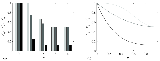
Figure 1: For the $[[4,1,2]]$ code $\mathcal{G}_{4a}$ we plot (a) from left to right, the transmission fidelity on $m$ qubits under error detection $\mathcal{F}^{\scriptscriptstyle d}_{m}$ [Eq. (81)] (light), the transmission fidelity on $m$ qubits under error correction $\mathcal{F}^{\scriptscriptstyle c}_{m}$ [Eq. (130)] (dark), the transmission rate on $m$ qubits under error detection $\mathcal{T}^{\scriptscriptstyle d}_{m}$ [Eq. (69)] (black), and (b) from top to bottom, $\mathcal{F}^{\scriptscriptstyle d}_{p}$ [Eq. (82)] (light), $\mathcal{F}^{\scriptscriptstyle c}_{p}$ [Eq. (131)] (dark), and $\mathcal{T}^{\scriptscriptstyle d}_{p}$ [Eq. (70)] (black) for the depolarizing channel.

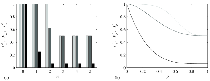
Figure 2: For the $[[5,1,3]]$ code $\mathcal{G}_{5}$ we plot (a) from left to right, the transmission fidelity on $m$ qubits under error detection $\mathcal{F}^{\scriptscriptstyle d}_{m}$ [Eq. (81)] (light), the transmission fidelity on $m$ qubits under error correction $\mathcal{F}^{\scriptscriptstyle c}_{m}$ [Eq. (130)] (dark), the transmission rate on $m$ qubits under error detection $\mathcal{T}^{\scriptscriptstyle d}_{m}$ [Eq. (69)] (black), and (b) from top to bottom, $\mathcal{F}^{\scriptscriptstyle d}_{p}$ [Eq. (82)] (light), $\mathcal{F}^{\scriptscriptstyle c}_{p}$ [Eq. (131)] (dark), and $\mathcal{T}^{\scriptscriptstyle d}_{p}$ [Eq. (70)] (black) for the depolarizing channel.

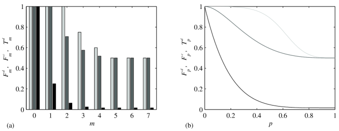
Figure 3: For Steane’s $[[7,1,3]]$ code $\mathcal{G}_{7b}$ we plot (a) from left to right, the transmission fidelity on $m$ qubits under error detection $\mathcal{F}^{\scriptscriptstyle d}_{m}$ [Eq. (81)] (light), the transmission fidelity on $m$ qubits under error correction $\mathcal{F}^{\scriptscriptstyle c}_{m}$ [Eq. (130)] (dark), the transmission rate on $m$ qubits under error detection $\mathcal{T}^{\scriptscriptstyle d}_{m}$ [Eq. (69)] (black), and (b) from top to bottom, $\mathcal{F}^{\scriptscriptstyle d}_{p}$ [Eq. (82)] (light), $\mathcal{F}^{\scriptscriptstyle c}_{p}$ [Eq. (131)] (dark), and $\mathcal{T}^{\scriptscriptstyle d}_{p}$ [Eq. (70)] (black) for the depolarizing channel.

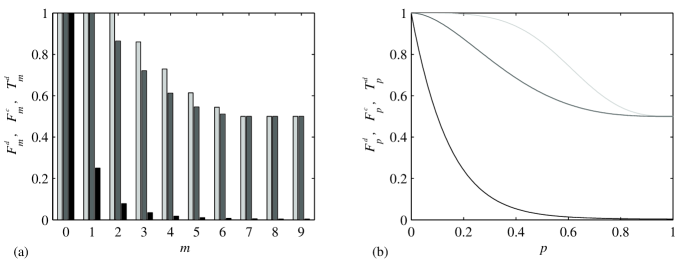
Figure 4: For Shor’s $[[9,1,3]]$ code $\mathcal{G}_{9c}$ we plot (a) from left to right, the transmission fidelity on $m$ qubits under error detection $\mathcal{F}^{\scriptscriptstyle d}_{m}$ [Eq. (81)] (light), the transmission fidelity on $m$ qubits under error correction $\mathcal{F}^{\scriptscriptstyle c}_{m}$ [Eq. (130)] (dark), the transmission rate on $m$ qubits under error detection $\mathcal{T}^{\scriptscriptstyle d}_{m}$ [Eq. (69)] (black), and (b) from top to bottom, $\mathcal{F}^{\scriptscriptstyle d}_{p}$ [Eq. (82)] (light), $\mathcal{F}^{\scriptscriptstyle c}_{p}$ [Eq. (131)] (dark), and $\mathcal{T}^{\scriptscriptstyle d}_{p}$ [Eq. (70)] (black) for the depolarizing channel.

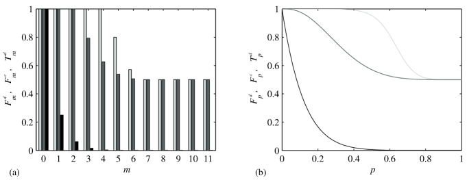
Figure 5: For the $[[11,1,5]]$ code $\mathcal{G}_{11}$ we plot (a) from left to right, the transmission fidelity on $m$ qubits under error detection $\mathcal{F}^{\scriptscriptstyle d}_{m}$ [Eq. (81)] (light), the transmission fidelity on $m$ qubits under error correction $\mathcal{F}^{\scriptscriptstyle c}_{m}$ [Eq. (130)] (dark), the transmission rate on $m$ qubits under error detection $\mathcal{T}^{\scriptscriptstyle d}_{m}$ [Eq. (69)] (black), and (b) from top to bottom, $\mathcal{F}^{\scriptscriptstyle d}_{p}$ [Eq. (82)] (light), $\mathcal{F}^{\scriptscriptstyle c}_{p}$ [Eq. (131)] (dark), and $\mathcal{T}^{\scriptscriptstyle d}_{p}$ [Eq. (70)] (black) for the depolarizing channel.

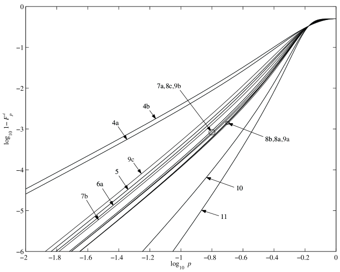
Figure 6: The transmission fidelity for the depolarizing channel under error detection $\mathcal{F}^{\scriptscriptstyle d}_{p}$ [Eq. (82)].

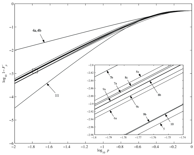
Figure 7: The transmission fidelity for the depolarizing channel under error correction $\mathcal{F}^{\scriptscriptstyle c}_{p}$ [Eq. (131)].

Unlike in the previous cases, an exhaustive search over all correction operators $C_{\lambda}\in\mathcal{E}_{\lambda}$ is required to calculate the transmission fidelities $\mathcal{F}^{\scriptscriptstyle c}_{m}(P)$ and $\mathcal{F}^{\scriptscriptstyle c}_{p}(P)$. Although it is not apparent from Eq. (130), given an $[[n,k,d]]_{D}$ code, $\mathcal{F}^{\scriptscriptstyle c}_{m}(P)=1$ for all $0\leq m<d/2$. In these cases we can choose $C_{\lambda}\in\mathcal{E}_{\lambda}$ to be of lowest weight in the set, and constant for all $0\leq m<d/2$. However, when $m\geq d/2$ (or when $p$ is large for $\mathcal{F}^{\scriptscriptstyle c}_{p}$) there may be more optimal choices. One example is the code generated by $\mathcal{G}_{7a}$ in the following section. Note from Eq.’s (96) and (126) that for stabilizer codes

$$A_{S}^{\prime}(FP) = \frac{1}{D^{|S|}D^{\prime}}\left|\left\{E\in F\mathcal{S}\,\big{|}\,\operatorname{supp}E\subseteq S\right\}\right|$$ (136)

$$A_{m}(FP) = \frac{1}{D^{\prime}}\left|\left\{E\in F\mathcal{S}\,\big{|}\,\operatorname{wt}E=S\right\}\right|$$ (137)

when $F\in\mathcal{E}$, and from either of which we can calculate $A_{m}^{\prime}(FP)$.

We may also define the probability of failure under error correction. The failure rate on qudits $S$ under error correction,

$$\mathscr{F}^{\scriptscriptstyle c}_{S}(P)\equiv 1-\mathcal{F}^{\scriptscriptstyle c}_{S}(P)=\frac{K\left[B_{S}^{\prime}(P)-A_{S}^{\prime}(P)\right]}{(K+1)B_{S}^{\prime}(P)},$$ (138)

and similarly, the failure rate on $m$ qudits under error correction is $\mathscr{F}^{\scriptscriptstyle c}_{m}(P)\equiv 1-\mathcal{F}^{\scriptscriptstyle c}_{m}(P)$, and the failure rate for the depolarizing channel under error correction is $\mathscr{F}^{\scriptscriptstyle c}_{p}(P)\equiv 1-\mathcal{F}^{\scriptscriptstyle c}_{p}(P)$.

Finally, to investigate the fidelity when $p$ is small, we set each $C_{\lambda}=C_{\lambda}(p)$, the optimal correction operator used for the maximization in Eq. (131). Now given that $\mathcal{F}^{\scriptscriptstyle c}_{m}(P)=1$ for all $0\leq m<d^{\prime}\equiv\lceil d/2\rceil$, when $p$ is small enough the operators $C_{\lambda}(p)$ may also be used for the maximizations in Eq. (130) ($0\leq m<d^{\prime}$). Thus, we must have

$$\sum_{\lambda}A_{m}^{\prime}\left(C_{\lambda}(p)P\right)=\frac{n!}{m!(n-m)!D^{n}}$$ (139)

for all $0\leq m<d^{\prime}$, when $p$ is small enough. Setting $C_{\lambda}^{\prime}=\lim_{p\rightarrow 0}C_{\lambda}(p)$, we have

$$\mathcal{F}^{\scriptscriptstyle c}_{p}(P) = 1-\frac{K}{K+1}\left\{1-\sum_{m=0}^{n}p^{m}(1-p)^{n-m}D^{-m}\sum_{\lambda}A_{m}^{\prime}\left(C_{\lambda}^{\prime}P\right)\right\}$$ (140)

$$= 1-\frac{K}{K+1}\left\{\sum_{m=0}^{n}p^{m}(1-p)^{n-m}\left[\frac{n!}{m!(n-m)!}-D^{-m}\sum_{\lambda}A_{m}^{\prime}\left(C_{\lambda}^{\prime}P\right)\right]\right\}$$ (141)

$$= 1-\frac{K}{K+1}\left\{\sum_{m=m^{\prime}}^{n}p^{m}(1-p)^{n-m}\left[\frac{n!}{m!(n-m)!}-D^{-m}\sum_{\lambda}A_{m}^{\prime}\left(C_{\lambda}^{\prime}P\right)\right]\right\}$$ (142)

$$= 1-\frac{K}{K+1}\left[\frac{n!}{d^{\prime}!(n-d^{\prime})!}-D^{-d^{\prime}}\sum_{\lambda}A_{d^{\prime}}^{\prime}\left(C_{\lambda}^{\prime}P\right)\right]p^{d^{\prime}}+O\left(p^{d^{\prime}+1}\right)$$ (143)

in the limit $p\rightarrow 0$. Consequently, for error correction, we define

$$c^{\prime}\equiv\frac{K}{K+1}\left[\frac{n!}{d^{\prime}!(n-d^{\prime})!}-D^{-d^{\prime}}\sum_{\lambda}A_{d^{\prime}}^{\prime}\left(C_{\lambda}^{\prime}P\right)\right].$$ (144)

If the operators $C_{\lambda}^{\prime}$ can also be used for the maximization in Eq. (130) when $m=d^{\prime}$, then $c^{\prime}=n!\mathscr{F}^{\scriptscriptstyle c}_{d^{\prime}}(P)/d!(n-d)!$. In all examples in the following section this was the case.

V Examples of stabilizer codes for qubits

A classical additive code over $GF(4)$ of length $n$ is an additive subgroup $\mathcal{C}$ of $GF(4)^{n}$. In the case of qubits, stabilizer codes correspond to classical additive codes over $GF(4)$ calderbank . This is shown as follows. Letting $GF(4)=\{0,1,\omega,\overline{\omega}\}$ where $\overline{\omega}=\omega^{2}=1+\omega$, we define the conjugate of $x\in GF(4)$, denoted $\overline{x}$, by the mapping $\overline{0}=0$, $\overline{1}=1$, and $\overline{\overline{\omega}}=\omega$. Next define the trace map $\operatorname{Tr}:GF(4)\rightarrow GF(2)$ by $\operatorname{Tr}(x)=x+x^{2}$ i.e. $\operatorname{Tr}(0)=\operatorname{Tr}(1)=0$ and $\operatorname{Tr}(\omega)=\operatorname{Tr}(\overline{\omega})=1$, and the trace inner product of two vectors ${\bf x}=x_{1}\dots x_{n}$ and ${\bf y}=y_{1}\dots y_{n}$ in $GF(4)^{n}$ as

$${\bf x\star y}=\sum_{i=1}^{n}\operatorname{Tr}\big{(}x_{i}\overline{y_{i}}\big{)}\;\;\in GF(2).$$ (145)

The weight $\operatorname{wt}({\bf x})$ of ${\bf x}\in GF(4)^{n}$ is the number of nonzero components of ${\bf x}$, and the minimum weight of a code $\mathcal{C}$ is the smallest weight of any nonzero codeword in $\mathcal{C}$. Next, by defining the mapping $\Phi:GF(4)^{n}\rightarrow\mathcal{E}$ by $\Phi({\bf x})=\mathcal{D}(\phi^{-1}({\bf x}))$ where $\phi(\bm{\mu},\bm{\nu})=\omega\bm{\mu}+\overline{\omega}\bm{\nu}$, we can associate elements of $GF(4)$ with Pauli matrices ($\omega\rightarrow X$, $\overline{\omega}\rightarrow Z$, $1\rightarrow iXZ$, $0\rightarrow I$), addition of vectors over $GF(4)^{n}$ with multiplication of operators in $\mathcal{E}$ (neglecting phases), and the trace inner product on $GF(4)^{n}$ with the commutator on $\mathcal{E}$.

If $\mathcal{C}$ is an additive code, its dual is the additive code $\mathcal{C}^{\perp}=\{{\bf x}\in GF(4)^{n}\,|\,{\bf x\star c}=0\;\forall\,{\bf c}\in\mathcal{C}\}$. The code $\mathcal{C}$ is called self-orthogonal if $\mathcal{C}\subseteq\mathcal{C}^{\perp}$ and self-dual if $\mathcal{C}=\mathcal{C}^{\perp}$. The following theorem now applies calderbank : Suppose $\mathcal{C}$ is a self-orthogonal additive subgroup of $GF(4)^{n}$, containing $2^{n-k}$ vectors, such that there are no vectors of weight $<d$ in $\mathcal{C}^{\perp}\backslash\mathcal{C}$. Then any joint eigenspace of $\Phi(\mathcal{C})$ is an $[[n,k,d]]$ quantum error-correcting code.

We say that $\mathcal{C}$ is pure if there are no nonzero vectors of weight $<d$ in $\mathcal{C}^{\perp}$. The associated quantum code is then pure if and only if $\mathcal{C}$ is pure. By convention, an $[[n,0,d]]$ code corresponds to a self-dual additive code $\mathcal{C}$ with minimum weight $d$. Such codes are thus always pure.

The weight enumerators of an additive code $\mathcal{C}$ are the Shor-Laflamme weight enumerators [Eq.’s (53) and (54)] for the corresponding quantum code

$$A_{m}(P) = A_{m}(\mathcal{C})\equiv|\{{\bf x}\in\mathcal{C}\,|\,\operatorname{wt}({\bf x})=m\}|$$ (146)

$$B_{m}(P) = B_{m}(\mathcal{C})\equiv|\{{\bf x}\in\mathcal{C^{\perp}}\,|\,\operatorname{wt}({\bf x})=m\}|.$$ (147)

The Rains enumerators may then be found through Eq.’s (55) and (56), or through their definition [Eq.’s (45) and (46)] with

$$A_{S}^{\prime}(P) = A_{S}^{\prime}(\mathcal{C})\equiv\frac{1}{2^{|S|}}|\{{\bf x}\in\mathcal{C}\,|\,\operatorname{supp}({\bf x})\subseteq S\}|$$ (148)

$$B_{S}^{\prime}(P) = B_{S}^{\prime}(\mathcal{C})\equiv\frac{1}{2^{|S|}}|\{{\bf x}\in\mathcal{C^{\perp}}\,|\,\operatorname{supp}({\bf x})\subseteq S\}|$$ (149)

where $\operatorname{supp}({\bf x})$ is the subset of $\{1,\dots,n\}$ consisting of all indices labeling a nonzero component of ${\bf x}$. Finally, note that when $\Phi({\bf y})=F$ we have

$$A_{S}^{\prime}(FP) = A_{S}^{\prime}({\bf y}+\mathcal{C})\equiv\frac{1}{2^{|S|}}|\{{\bf x}\in{\bf y}+\mathcal{C}\,|\,\operatorname{supp}({\bf x})\subseteq S\}|$$ (150)

$$A_{m}(FP) = A_{m}({\bf y}+\mathcal{C})\equiv|\{{\bf x}\in{\bf y}+\mathcal{C}\,|\,\operatorname{wt}({\bf x})\subseteq S\}|.$$ (151)

The advantage of making the above correspondence is that a wealth of classical coding theory immediately becomes available. Indeed the classical Hamming code with generator matrix

$$\mathcal{G}_{5}=\left[\begin{array}[]{ccccc}\omega&\overline{\omega}&\overline{\omega}&\omega&0\\ 0&\omega&\overline{\omega}&\overline{\omega}&\omega\\ \omega&0&\omega&\overline{\omega}&\overline{\omega}\\ \overline{\omega}&\omega&0&\omega&\overline{\omega}\end{array}\right]$$ (152)

gives the quantum $[[5,1,3]]$ code. The rows of the generator matrix define a basis (under addition) for the classical code $\mathcal{C}$, and, with the above correspondence, define generators (up to a phase) for the stabilizer $\mathcal{S}$ in the quantum version.

Two additive codes $\mathcal{C}_{1}$ and $\mathcal{C}_{2}$ are said to be equivalent when there exists a map between codewords of $\mathcal{C}_{1}$ and codewords of $\mathcal{C}_{2}$ consisting of a permutation of coordinates, a scaling of coordinates by elements of $GF(4)$, and conjugation of some of the coordinates. The quantum Hamming code above is unique under equivalence. We now catalogue other inequivalent additive codes whose quantum analogues encode a single qubit i.e. $k=1$.

Exhaustive searches show that

$$\mathcal{G}_{4a}=\left[\begin{array}[]{cccc}0&\overline{\omega}&\omega&\overline{\omega}\\ 1&\omega&\omega&1\\ \omega&\overline{\omega}&\overline{\omega}&\omega\end{array}\right],\qquad\mathcal{G}_{4b}=\left[\begin{array}[]{cccc}\omega&\omega&\omega&\omega\\ \overline{\omega}&\overline{\omega}&0&0\\ 0&0&\overline{\omega}&\overline{\omega}\end{array}\right],$$ (153)

and

$$\mathcal{G}_{6a}=\left[\begin{array}[]{cccccc}0&0&0&0&1&1\\ 0&1&1&1&1&0\\ 0&\omega&\omega&\omega&\omega&\omega\\ 1&0&1&\omega&\overline{\omega}&\omega\\ \omega&0&\omega&\overline{\omega}&1&0\end{array}\right],\qquad\mathcal{G}_{6b}=1\oplus\mathcal{G}_{5}\>,$$ (154)

generate, respectively, the only inequivalent $[[4,1,2]]$ and $[[6,1,3]]$ codes calderbank . The 4-qubit codes are pure while the 6-qubit codes are necessarily impure. The code generated by $\mathcal{G}_{6b}$ offers no advantage over the 5-qubit code and will not be investigated any further.

Rows of the matrices

$$\mathcal{G}_{7a}=\left[\begin{array}[]{ccccccc}0&0&0&1&1&1&1\\ 0&0&1&0&\omega&\overline{\omega}&1\\ 0&1&0&\omega&\overline{\omega}&\overline{\omega}&\omega\\ 0&\omega&\omega&\omega&1&\overline{\omega}&0\\ 1&0&0&0&\overline{\omega}&\omega&1\\ \omega&0&\omega&\omega&\overline{\omega}&\omega&\overline{\omega}\end{array}\right],\qquad\mathcal{G}_{7b}=\left[\begin{array}[]{ccccccc}0&0&0&\omega&\omega&\omega&\omega\\ 0&\omega&\omega&0&0&\omega&\omega\\ \omega&0&\omega&0&\omega&0&\omega\\ 0&0&0&\overline{\omega}&\overline{\omega}&\overline{\omega}&\overline{\omega}\\ 0&\overline{\omega}&\overline{\omega}&0&0&\overline{\omega}&\overline{\omega}\\ \overline{\omega}&0&\overline{\omega}&0&\overline{\omega}&0&\overline{\omega}\end{array}\right],$$ (155)

generate inequivalent $[[7,1,3]]$ codes. These may be found by puncturing (Theorem 6b of calderbank ) the extremal self-dual additive codes of length 8 found by Gaborit et al gaborit . Both codes are pure. The code generated by $\mathcal{G}_{7b}$ is the Steane code steane . More inequivalent $[[7,1,3]]$ codes will exist. For example, we can always trivially extend lower dimensional codes as done in the case of $\mathcal{G}_{6b}$.

Examples of $[[8,1,3]]$ codes follow from the matrices

$$\mathcal{G}_{8a}=\left[\begin{array}[]{cccccccc}0&0&0&1&1&1&1&1\\ 0&0&0&\omega&\omega&\omega&\omega&0\\ 0&0&1&0&1&\omega&1&\overline{\omega}\\ 0&1&0&0&\omega&\overline{\omega}&\overline{\omega}&\omega\\ 0&\omega&\omega&0&1&0&1&1\\ 1&0&0&0&0&1&\overline{\omega}&\overline{\omega}\\ \omega&0&\omega&0&\overline{\omega}&1&0&\omega\end{array}\right],\qquad\mathcal{G}_{8b}=\left[\begin{array}[]{cccccccc}0&0&0&1&1&\overline{\omega}&\omega&0\\ 0&0&1&0&\omega&\omega&0&1\\ 0&0&\omega&\omega&0&\omega&0&\omega\\ 0&1&0&0&0&1&\overline{\omega}&\overline{\omega}\\ 0&\omega&0&\omega&\omega&1&1&\overline{\omega}\\ 1&0&0&0&\overline{\omega}&0&1&\omega\\ \omega&0&0&\omega&0&\omega&\omega&0\end{array}\right],$$ (156)

$$\mathcal{G}_{8c}=\left[\begin{array}[]{cccccccc}0&0&0&1&1&1&1&1\\ 0&0&0&\omega&\omega&\omega&\omega&0\\ 0&0&1&0&1&\overline{\omega}&\omega&0\\ 0&1&0&0&\omega&\omega&0&1\\ 0&\omega&\omega&0&0&\omega&0&\omega\\ 1&0&0&0&0&1&\overline{\omega}&\overline{\omega}\\ \omega&0&\omega&0&\omega&1&1&\overline{\omega}\end{array}\right].$$ (157)

All of these codes are pure and were found by puncturing the extremal self-dual additive codes of length 9 in gaborit . Again, more inequivalent $[[8,1,3]]$ codes will exist.

Examples of $[[9,1,3]]$ codes include

$$\mathcal{G}_{9a}=\left[\begin{array}[]{ccccccccc}0&0&0&0&\omega&\overline{\omega}&\overline{\omega}&0&\overline{\omega}\\ 0&0&0&1&0&1&0&1&1\\ 0&0&1&0&1&0&0&1&1\\ 0&0&\omega&\omega&0&0&\overline{\omega}&\overline{\omega}&0\\ 0&1&0&0&1&0&1&1&0\\ 0&\omega&0&\omega&0&\overline{\omega}&\overline{\omega}&0&0\\ 1&0&0&0&0&1&1&1&0\\ \omega&0&0&\omega&1&\omega&\omega&\omega&\omega\end{array}\right],\qquad\mathcal{G}_{9b}=\left[\begin{array}[]{ccccccccc}0&0&0&0&\omega&0&1&1&\omega\\ 0&0&0&1&1&1&1&1&1\\ 0&0&0&\omega&0&\omega&\overline{\omega}&\overline{\omega}&0\\ 0&0&1&0&0&1&\omega&0&\overline{\omega}\\ 0&1&0&0&0&1&0&\omega&\overline{\omega}\\ 0&\omega&\omega&0&0&\overline{\omega}&1&\overline{\omega}&1\\ 1&0&0&0&1&1&1&\overline{\omega}&\omega\\ \omega&0&\omega&0&1&\overline{\omega}&0&1&\overline{\omega}\end{array}\right],$$ (158)

$$\mathcal{G}_{9c}=\left[\begin{array}[]{ccccccccc}\overline{\omega}&\overline{\omega}&0&0&0&0&0&0&0\\ 0&\overline{\omega}&\overline{\omega}&0&0&0&0&0&0\\ 0&0&0&\overline{\omega}&\overline{\omega}&0&0&0&0\\ 0&0&0&0&\overline{\omega}&\overline{\omega}&0&0&0\\ 0&0&0&0&0&0&\overline{\omega}&\overline{\omega}&0\\ 0&0&0&0&0&0&0&\overline{\omega}&\overline{\omega}\\ \omega&\omega&\omega&\omega&\omega&\omega&0&0&0\\ 0&0&0&\omega&\omega&\omega&\omega&\omega&\omega\end{array}\right].$$ (159)

The first two codes, $\mathcal{G}_{9a}$ and $\mathcal{G}_{9b}$, are pure and were found by puncturing the extremal self-dual additive codes of length 10 found by Bachoc and Gaborit bachoc . The code generated by $\mathcal{G}_{9c}$ is the impure Shor code shor2 . Many more inequivalent $[[9,1,3]]$ codes will exist.

Finally we give generator matrices for pure $[[10,1,4]]$ and $[[11,1,5]]$ codes, found by puncturing, respectively, the shortened dodecacode and dodecacode:

$$\mathcal{G}_{10}=\left[\begin{array}[]{cccccccccc}\omega&0&0&0&0&\overline{\omega}&\omega&\omega&\overline{\omega}&0\\ 0&\omega&0&0&\overline{\omega}&1&\omega&\overline{\omega}&\overline{\omega}&\omega\\ 0&0&\omega&0&0&\overline{\omega}&1&\overline{\omega}&\overline{\omega}&\omega\\ 0&0&0&\omega&\overline{\omega}&1&1&1&\omega&1\\ 0&0&0&0&\omega&\overline{\omega}&0&\overline{\omega}&1&1\\ 0&\overline{\omega}&0&0&0&\omega&1&1&1&1\\ 0&0&\overline{\omega}&0&\overline{\omega}&0&\omega&\omega&\overline{\omega}&\overline{\omega}\\ \overline{\omega}&\overline{\omega}&\overline{\omega}&0&\overline{\omega}&0&\overline{\omega}&\omega&0&1\\ \overline{\omega}&0&0&\overline{\omega}&0&0&\overline{\omega}&\overline{\omega}&\omega&\omega\end{array}\right],\qquad\mathcal{G}_{11}=\left[\begin{array}[]{ccccccccccc}\omega&0&0&0&0&\overline{\omega}&\overline{\omega}&\overline{\omega}&0&\omega&\omega\\ 0&\omega&0&0&0&\overline{\omega}&\overline{\omega}&1&\overline{\omega}&0&1\\ 0&0&\omega&0&0&\overline{\omega}&\overline{\omega}&\omega&\omega&\overline{\omega}&0\\ 0&0&0&\omega&0&\overline{\omega}&1&0&\omega&\omega&1\\ 0&0&0&0&\omega&\overline{\omega}&\omega&0&\overline{\omega}&\overline{\omega}&\omega\\ 0&0&\overline{\omega}&0&0&\omega&1&0&1&\overline{\omega}&\overline{\omega}\\ 0&\overline{\omega}&\overline{\omega}&0&0&0&\omega&\overline{\omega}&0&\omega&\overline{\omega}\\ 0&\overline{\omega}&0&0&\overline{\omega}&0&\overline{\omega}&\omega&\omega&0&\overline{\omega}\\ \overline{\omega}&\overline{\omega}&\overline{\omega}&0&\overline{\omega}&0&0&\overline{\omega}&\omega&\overline{\omega}&\omega\\ 0&\overline{\omega}&0&\overline{\omega}&0&0&\overline{\omega}&0&\overline{\omega}&\omega&\omega\end{array}\right].$$ (160)

In Fig.’s 1 through 5 we plot the quantities $\mathcal{T}^{\scriptscriptstyle d}_{m}$, $\mathcal{F}^{\scriptscriptstyle d}_{m}$, $\mathcal{F}^{\scriptscriptstyle c}_{m}$, $\mathcal{T}^{\scriptscriptstyle d}_{p}$, $\mathcal{F}^{\scriptscriptstyle d}_{p}$, and $\mathcal{F}^{\scriptscriptstyle c}_{p}$ for the $[[4,1,2]]$ code $\mathcal{G}_{4a}$, the unique $[[5,1,3]]$ code $\mathcal{G}_{5}$, Stean’s $[[7,1,3]]$ code $\mathcal{G}_{7b}$, Shor’s impure $[[9,1,3]]$ code $\mathcal{G}_{9c}$, and the $[[11,1,5]]$ code $\mathcal{G}_{11}$. Next, in Fig.’s 6 and 7, we plot $\log_{10}1-\mathcal{F}^{\scriptscriptstyle d}_{p}$ and $\log_{10}1-\mathcal{F}^{\scriptscriptstyle c}_{p}$, respectively, versus $\log_{10}p$ for all of the stabilizer codes given above.

When $p$ is small the transmission fidelity under error detection follows from Eq. (92), and thus we can rank different codes using the pair $(d,c)$, where $c$ is defined in Eq. (93). The codes in order are: $\mathcal{G}_{4b}$ (2,1/3), $\mathcal{G}_{4a}$ (2,1/4), $\mathcal{G}_{9c}$ (3,13/32), $\mathcal{G}_{5}$ (3,5/16), $\mathcal{G}_{6a}$ (3,1/4), $\mathcal{G}_{7b}$ (3,7/32), $\mathcal{G}_{7a}$ (3,13/96),$\mathcal{G}_{8c}$ (3,1/8), $\mathcal{G}_{9b}$ (3,1/8), $\mathcal{G}_{8b}$ (3,1/12), $\mathcal{G}_{8a}$ (3,1/12),$\mathcal{G}_{9a}$ (3,1/12), $\mathcal{G}_{10}$ (4,5/64), and $\mathcal{G}_{11}$ (5,33/256). Note that as the number of qubits increases we are generally able to construct better codes even when the minimum distance remains constant. However this is not the case for error correction.

In the case of error correction we use the pair $(d^{\prime},c^{\prime})$ [see Eq.’s (143) and (144)] to rank different codes. The codes in order are now: $\mathcal{G}_{4b}$ (1,1), $\mathcal{G}_{4a}$ (1,1), $\mathcal{G}_{7b}$ (2,49/8), $\mathcal{G}_{8a}$ (2,127/24), $\mathcal{G}_{8c}$ (2,31/6), $\mathcal{G}_{7a}$ (2,41/8), $\mathcal{G}_{9a}$ (2,5), $\mathcal{G}_{8b}$ (2,5), $\mathcal{G}_{9c}$ (2,39/8), $\mathcal{G}_{6a}$ (2,19/4), $\mathcal{G}_{9b}$ (2,23/6), $\mathcal{G}_{10}$ (2,15/4), $\mathcal{G}_{5}$ (2,15/4), and $\mathcal{G}_{11}$ (3,273/8). Note that the 5-qubit code outperforms all other codes of minimum distance 3. The 10-qubit code asymptotes to the five only at much smaller values of $p$ than shown in the inset of Fig. 7. Thus, for the codes investigated, the benefit of accessing more qubits to construct a code is outweighed by the cost of allowing the extra qubits into an error-prone environment.

VI Conclusion

In conclusion, we have investigated the performance of a quantum error-correcting code when stretched beyond its intended capabilities. The content of Theorem’s 70, 82 and 113, along with Proposition 131 form the main results of the paper. We have derived the transmission rate, $\mathcal{T}^{\scriptscriptstyle d}$ (the probability that no error is detected), and the transmission fidelity, $\mathcal{F}^{\scriptscriptstyle d}$, under error detection, in Theorem’s 70 and 82 respectively. In the error detection scenario a corrupted state is simply discarded once detected. Theorem 113 and Proposition 131 are concerned with error correction. Here we attempt to correct all corrupted states. In this case we give expressions for transmission fidelity, $\mathcal{F}^{\scriptscriptstyle c}$, for stabilizer codes. The quantities $\mathcal{F}^{\scriptscriptstyle c}$, $\mathcal{F}^{\scriptscriptstyle d}$ and $\mathcal{T}^{\scriptscriptstyle d}$ in their various forms, or $c$ and $c^{\prime}$ [Eq.s (93) and (144)], might be used to compare different quantum error-correcting codes of the same minimum distance. Indeed, under the depolarizing channel, the unique five-qubit quantum Hamming code outperforms other known codes of the same minimum distance in the error correction scenario, but loses out to codes constructed from higher numbers of qubits in the error detection scenario.

References

(1)A. R. Calderbank, E. M. Rains, P. W. Shor, and N. J. A. Sloane, IEEE Trans. Inform. Theory 44, 1369 (1998).
(2)D. Gottesman, PhD Thesis (California Institute of Technology, Pasadena CA, 1997); e-print quant-ph/9705052.
(3)E. Knill and R. Laflamme, Phys. Rev. A 55, 900 (1997).
(4)J. Preskill, Lecture notes for Physics 219: Quantum Computation (California Institute of Technology, Pasadena CA, 1998).
URL: http://www.theory.caltech.edu/people/preskill/ph219/
(5)M. A. Nielsen and I. L. Chuang, Quantum Computation and Quantum Information (Cambridge University Press, Cambridge, 2000).
(6)M. Grassl, in Mathematics of Quantum Computation, edited by R. K. Brylinski and G. Chen (Chapman & Hall / CRC, London, 2002).
(7)P. Shor, Phys. Rev. A 52, 2493 (1995).
(8)A. M. Steane, Phys. Rev. Lett. 77, 793 (1996).
(9)A. E. Ashikhmin, A. M. Barg, E. Knill, and S. N. Litsyn, IEEE Trans. Inform. Theory 46, 778 (2000).
(10)E. M. Rains, IEEE Trans. Inform. Theory 44, 1388 (1998).
(11)P. Shor and R. Laflamme, Phys. Rev. Lett. 78, 1600 (1997).
(12)E. M. Rains, IEEE Trans. Inform. Theory 45, 1827 (1999).
(13)A. Ashikhmin and E. Knill, IEEE Trans. Inform. Theory 47, 3065 (2001).
(14)M. Grassl, T. Beth, and M. Rötteler, Int. J. Quantum Inf. 2, 55 (2004).
(15)P. Gaborit, W. C. Huffman, J.-L. Kim, and V. Pless, in DIMACS Series in Discrete Mathematics and Theoretical Computer Science Volume 56: Codes and Association Schemes, edited by A. Barg and S. Litsyn (American Mathematical Society, Providence RI, 2001).
(16)C. Bachoc and P. Gaborit, Journal de Théorie des Nombres de Bordeaux 12, 255 (2000); Electronic Notes in Discrete Mathematics 6, (2001).