Abstract

An experiment that involves two distant mesoscopic SQUID rings is studied. The superconducting rings are irradiated with correlated photons, which are produced by a single microwave source. Classically correlated (separable) and quantum mechanically correlated (entangled) microwaves are considered, and their effect on the Josephson currents is quantified. It is shown that the currents tunnelling through the Josephson junctions in the distant rings, are correlated.

[Entanglement of distant SQUID rings]Photon-induced entanglement of distant mesoscopic SQUID rings

1 Introduction

A fundamental property of superconducting quantum interference devices (SQUIDs) is that they exhibit quantum coherence at the macroscopic level [1]. This property may be used for the purposes of quantum information processing [2, 3].

A lot of research on superconducting devices investigates their interaction with classical microwaves. On the other hand the use of nonclassical microwaves makes the system fully quantum mechanical and interesting quantum phenomena arise. For example, in this paper we show that entangled two-mode microwaves produce correlated currents in distant SQUID rings.

Nonclassical electromagnetic fields at low temperatures ($k_{\rm B}T\ll\hbar\omega$) have been studied for more than twenty years both theoretically and experimentally [4]. The interaction of SQUID rings with nonclassical microwaves has been studied in the literature [5, 6].

In previous publications [7] we have studied the effects of entangled electromagnetic fields on distant electron interference experiments. In this paper we review and extend further this work in the context of SQUID rings. We consider two mesoscopic SQUID rings, which are far from each other and are irradiated with entangled microwaves, produced by a single source (Fig. 1). It is shown that the Josephson currents in the distant SQUID rings are correlated. The photon-induced correlations between the currents are quantified. It is shown that the current correlations depend on whether the photons are classically correlated (separable) or quantum mechanically correlated (entangled). The difference between separable and entangled microwave density matrices [8] is in the nondiagonal elements; and the effect of these nondiagonal elements on the Josephson currents is explicitly calculated.

2 Interaction of a single SQUID ring with nonclassical microwaves

In this section we consider a single SQUID ring and study its interaction with both classical and nonclassical microwaves.

For irradiation with classical microwaves, the Josephson current is $I_{\rm A}=I_{1}\sin\theta_{\rm A}$, where $\theta_{\rm A}=2e\Phi_{\rm A}$ is the phase difference across the junction due to the total flux $\Phi_{\rm A}$ through the ring. We assume the external field approximation, where the back reaction (the additional flux induced by the SQUID ring current) is neglected; i.e., the flux ${\cal L}I_{\rm A}$, where ${\cal L}$ is the self-inductance of the ring, is negligible in comparison to $\Phi_{\rm A}$. The magnetic flux has a linear and a sinusoidal component:

$$\Phi_{\rm A}=V_{\rm A}t+\phi_{\rm A};\;\;\;\;\;\phi_{\rm A}=A\sin(\omega_{1}t).$$ (1)

Consequently the observed current is

$$I_{\rm A}=I_{1}\sin[\omega_{\rm A}t+2eA\sin(\omega_{1}t)];\;\;\;\;\;\omega_{\rm A}=2eV_{\rm A}.$$ (2)

We now consider the interaction of a SQUID ring with nonclassical microwaves, that are carefully prepared in a particular quantum state and are described by a density matrix $\rho$. The dual quantum variables of the nonclassical field are the vector potential $A_{i}$ and the electric field $E_{i}$. Integrating these over the SQUID ring we obtain the magnetic flux and the electromotive force operators $\hat{\phi}=\oint_{C}A_{i}dx_{i}$, $\hat{V}_{\rm EMF}=\oint_{C}E_{i}dx_{i}$.

In the external field approximation the flux operator evolves as

$$\hat{\phi}(t)=\xi 2^{-1/2}[\hat{a}^{\dagger}\exp(i\omega t)+\hat{a}\exp(-i\omega t)],$$ (3)

where $\xi$ is a parameter proportional to the area of the SQUID ring and the $\hat{a}^{\dagger},\hat{a}$ are the photon creation and annihilation operators. Consequently the phase difference $\theta_{\rm A}$ is the operator

$$\hat{\theta}_{\rm A}=\omega_{\rm A}t+q[{\hat{a}}^{\dagger}\exp(i\omega t)+\hat{a}\exp(-i\omega t)],\;\;\;\;\;q=\sqrt{2}e\xi;$$ (4)

and the current also becomes an operator, $\hat{I}_{\rm A}=I_{1}\sin\hat{\theta}_{\rm A}$. Expectation values of the current are calculated by taking its trace with respect to the density matrix $\rho$, which describes the nonclassical electromagnetic fields,

$$\langle\hat{I}_{\rm A}\rangle = \mbox{Tr}(\rho\hat{I}_{\rm A})=I_{1}\mbox{Im}[\exp(i\omega_{\rm A}t)\tilde{W}(\lambda_{\rm A})],$$ (5)

$$\lambda_{\rm A} = iq\exp(i\omega_{1}t).$$ (6)

$\tilde{W}(x)$ is the Weyl function [9] given by

$$\tilde{W}(x)=\mbox{Tr}[\rho D(x)];\;\;\;\;\;D(x)=\exp(x\hat{a}^{\dagger}-x^{*}\hat{a})$$ (7)

where $D(x)$ is the displacement operator. Higher moments of the Josephson current quantify the quantum statistics of the electron pairs tunnelling through the junction.

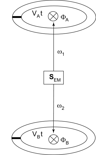
Figure 1: Two distant mesoscopic SQUID rings A and B are irradiated with nonclassical microwaves of frequencies $\omega_{1}$ and $\omega_{2}$, correspondingly. The microwaves are produced by the source ${\rm S}_{\rm EM}$ and are correlated. Classical magnetic fluxes $V_{\rm A}t$ and $V_{\rm B}t$ are also threading the two rings A and B, correspondingly.

3 Interaction of two distant SQUID rings with entangled microwaves

In this section we consider two mesoscopic SQUID rings far apart from each other, which we refer to as A and B (Fig. 1). They are irradiated with correlated microwaves. Let $\rho$ be the density matrix of the microwaves, and $\rho_{\rm A}={\rm Tr}_{\rm B}\rho$, $\rho_{\rm B}={\rm Tr}_{\rm A}\rho$, the density matrices of the microwaves interacting with the two SQUID rings ${\rm A}$, ${\rm B}$, correspondingly. When the density matrix $\rho$ is factorizable as $\rho_{\rm fact}=\rho_{\rm A}\otimes\rho_{\rm B}$ the two modes are not correlated. If it can be written as $\rho_{\rm sep}=\sum_{i}p_{i}\rho_{{\rm A}i}\otimes\rho_{{\rm B}i}$, where $p_{i}$ are probabilities, it is called separable and the two modes are classically correlated. Density matrices which cannot be written in one of these two forms are entangled (quantum mechanically correlated) [8].

The currents in the two SQUIDs are

$$\langle\hat{I}_{\rm A}\rangle=I_{1}\mbox{Tr}(\rho_{\rm A}\sin\hat{\theta}_{\rm A}),\;\;\;\;\;\langle\hat{I}_{\rm B}\rangle=I_{2}\mbox{Tr}(\rho_{\rm B}\sin\hat{\theta}_{\rm B}).$$ (8)

The expectation value of the product of the two current operators is given by:

$$\langle\hat{I}_{\rm A}\hat{I}_{\rm B}\rangle=I_{1}I_{2}\mbox{Tr}(\rho\sin\hat{\theta}_{\rm A}\sin\hat{\theta}_{\rm B}).$$ (9)

In general $\langle\hat{I}_{\rm A}\hat{I}_{\rm B}\rangle$ is different from $\langle\hat{I}_{\rm A}\rangle\langle\hat{I}_{\rm B}\rangle$ and we calculate the ratio

$$R=\frac{\langle\hat{I}_{\rm A}\hat{I}_{\rm B}\rangle}{\langle\hat{I}_{\rm A}\rangle\langle\hat{I}_{\rm B}\rangle}.$$ (10)

For factorizable density matrices $\rho_{\rm fact}=\rho_{A}\otimes\rho_{B}$ we easily see that $R_{\rm fact}=1$. For separable density matrices $\rho_{\rm sep}$ the ratio $R_{\rm sep}$ is not necessarily equal to one and numerical results for various examples are shown below.

We also calculate the second moments

$$\langle{\hat{I}}_{\rm A}^{2}\rangle=I_{1}^{2}\mbox{Tr}[\rho_{\rm A}(\sin\hat{\theta}_{\rm A})^{2}],\;\;\;\;\;\langle{\hat{I}}_{\rm B}^{2}\rangle=I_{2}^{2}\mbox{Tr}[\rho_{\rm B}(\sin\hat{\theta}_{\rm B})^{2}].$$ (11)

The statistics of the photons affects the statistics of the tunnelling electron pairs, which is quantified with the $\langle{\hat{I}}_{\rm A}{\hat{I}}_{\rm B}\rangle$, $\langle{\hat{I}}_{\rm A}^{2}\rangle$, $\langle{\hat{I}}^{2}_{\rm B}\rangle$ (and also with the higher moments).

3.1 Microwaves in number states

We consider microwaves in the separable (mixed) state

$$\rho_{\rm sep}=\frac{1}{2}(|N_{1}N_{2}\rangle\langle N_{1}N_{2}|+|N_{2}N_{1}\rangle\langle N_{2}N_{1}|),$$ (12)

where $N_{1}\neq N_{2}$. We also consider microwaves in the entangled state $|s\rangle=2^{-1/2}(|N_{1}N_{2}\rangle+|N_{2}N_{1}\rangle)$, which is a pure state. The density matrix of $|s\rangle$ is

$$\rho_{\rm ent}=\rho_{\rm sep}+\frac{1}{2}(|N_{1}N_{2}\rangle\langle N_{2}N_{1}|+|N_{2}N_{1}\rangle\langle N_{1}N_{2}|),$$ (13)

where the $\rho_{\rm sep}$ is given by Eq. (12). It is seen that the $\rho_{\rm ent}$ and the $\rho_{\rm sep}$ differ only by the above nondiagonal elements.

In this example, the reduced density matrices are the same for both the separable and entangled states:

$$\rho_{\rm sep,A}=\rho_{\rm ent,A}=\rho_{\rm sep,B}=\rho_{\rm ent,B}=\frac{1}{2}(|N_{1}\rangle\langle N_{1}|+|N_{2}\rangle\langle N_{2}|).$$ (14)

Consequently in this example $\langle\hat{I}_{\rm A}\rangle_{\rm sep}=\langle\hat{I}_{\rm A}\rangle_{\rm ent}$, and also $\langle\hat{I}_{\rm B}\rangle_{\rm sep}=\langle\hat{I}_{\rm B}\rangle_{\rm ent}$.

For the density matrix $\rho_{\rm sep}$ of Eq. (12) we find

$$\langle\hat{I}_{\rm A}\rangle = \frac{I_{1}}{2}\exp\left(-\frac{q^{2}}{2}\right)[L_{N_{1}}(q^{2})+L_{N_{2}}(q^{2})]\sin(\omega_{\rm A}t),$$ (15)

$$\langle\hat{I}_{\rm B}\rangle = \frac{I_{2}}{2}\exp\left(-\frac{q^{2}}{2}\right)[L_{N_{1}}(q^{2})+L_{N_{2}}(q^{2})]\sin(\omega_{\rm B}t),$$ (16)

where the $L_{n}^{\alpha}(x)$ are Laguerre polynomials. The currents $\langle\hat{I}_{\rm A}\rangle,\langle\hat{I}_{\rm B}\rangle$ are in this example independent of the microwave frequencies $\omega_{1},\omega_{2}$.

The expectation value of the product of the two currents [Eq. (9)] is

$$\langle{\hat{I}}_{\rm A}{\hat{I}}_{\rm B}\rangle_{\rm sep} = I_{1}I_{2}\exp(-q^{2})L_{N_{1}}(q^{2})L_{N_{2}}(q^{2})\sin(\omega_{\rm A}t)\sin(\omega_{\rm B}t).$$ (17)

Consequently the ratio $R$ of Eq. (10) is

$$R_{\rm sep}=\frac{4L_{N_{1}}(q^{2})L_{N_{2}}(q^{2})}{[L_{N_{1}}(q^{2})+L_{N_{2}}(q^{2})]^{2}}.$$ (18)

In this example the $R_{\rm sep}$ is time-independent.

The moments of the currents, defined by Eq. (11), are also calculated:

$$\langle\hat{I}_{\rm A}^{2}\rangle = \frac{I_{1}^{2}}{2}\left\{1-\frac{1}{2}\exp(-2q^{2})[L_{N_{1}}(4q^{2})+L_{N_{2}}(4q^{2})]\cos(2\omega_{\rm A}t)\right\},$$ (19)

$$\langle\hat{I}_{\rm B}^{2}\rangle = \frac{I_{2}^{2}}{2}\left\{1-\frac{1}{2}\exp(-2q^{2})[L_{N_{1}}(4q^{2})+L_{N_{2}}(4q^{2})]\cos(2\omega_{\rm B}t)\right\}.$$ (20)

For the case of $\rho_{\rm ent}$ the $\langle\hat{I}_{\rm A}\rangle,\langle\hat{I}_{\rm B}\rangle$ are the same as in Eqs. (15), (16); and the $\langle\hat{I}_{\rm A}^{2}\rangle,\langle\hat{I}_{\rm B}^{2}\rangle$ are the same as in Eqs. (19), (20). However the $\langle{\hat{I}}_{\rm A}{\hat{I}}_{\rm B}\rangle$ is

$$\langle{\hat{I}}_{\rm A}{\hat{I}}_{\rm B}\rangle_{\rm ent}=\langle{\hat{I}}_{\rm A}{\hat{I}}_{\rm B}\rangle_{\rm sep}+I_{\rm cross},$$ (21)

where

$$I_{\rm cross} = -\frac{I_{1}I_{2}}{2}\exp(-q^{2})L_{N_{1}}^{N_{2}-N_{1}}(q^{2})L_{N_{2}}^{N_{1}-N_{2}}(q^{2})[\cos(\omega_{\rm A}t+\omega_{\rm B}t)$$ (22)

$$-(-1)^{N_{1}-N_{2}}\cos(\omega_{\rm A}t-\omega_{\rm B}t)]\cos(\Omega t),$$

$$\Omega = (N_{1}-N_{2})(\omega_{1}-\omega_{2}).$$ (23)

It is seen that the effect of entangled microwaves on Josephson currents is different from the effect of separable microwaves. In this case the ratio $R$ of Eq. (10) is

$$R_{\rm ent}=R_{\rm sep}+\frac{I_{\rm cross}(t)}{\langle\hat{I}_{\rm A}\rangle\langle\hat{I}_{\rm B}\rangle},$$ (24)

which is a time-dependent quantity oscillating around the $R_{\rm sep}$.

3.2 Microwaves in coherent states

We consider microwaves in the classically correlated state

$$\rho_{{\rm sep}}=\frac{1}{2}(|A_{1}A_{2}\rangle\langle A_{1}A_{2}|+|A_{2}A_{1}\rangle\langle A_{2}A_{1}|),$$ (25)

where $|A_{1}\rangle$, $|A_{2}\rangle$ are microwave coherent states. We also consider the entangled state $|u\rangle={\cal N}(|A_{1}A_{2}\rangle+|A_{2}A_{1}\rangle)$, with density matrix

$$\rho_{\rm ent}=2{\cal N}^{2}\rho_{\rm sep}+{\cal N}^{2}(|A_{1}A_{2}\rangle\langle A_{2}A_{1}|+|A_{2}A_{1}\rangle\langle A_{1}A_{2}|),$$ (26)

where the normalization constant is given by

$${\cal N}=\left[2+2\exp\left(-|A_{1}-A_{2}|^{2}\right)\right]^{-1/2}.$$ (27)

For microwaves in the separable state of Eq. (25) the reduced density matrices are

$$\rho_{\rm sep,A}=\rho_{\rm sep,B}=\frac{1}{2}(|A_{1}\rangle\langle A_{1}|+|A_{2}\rangle\langle A_{2}|),$$ (28)

and hence the current in A is

$$\langle\hat{I}_{\rm A}\rangle_{\rm sep} = \frac{I_{1}}{2}\exp(-\frac{q^{2}}{2})\{\sin[\omega_{\rm A}t+2q|A_{1}|\cos(\omega_{1}t-\theta_{1})]$$ (29)

$$+ \sin[\omega_{\rm A}t+2q|A_{2}|\cos(\omega_{1}t-\theta_{2})]\}.$$

where $\theta_{1}=\arg(A_{1})$, and $\theta_{2}=\arg(A_{2})$. A similar expression yields the current in B. We have also calculated numerically the ratio $R_{\rm sep}$.

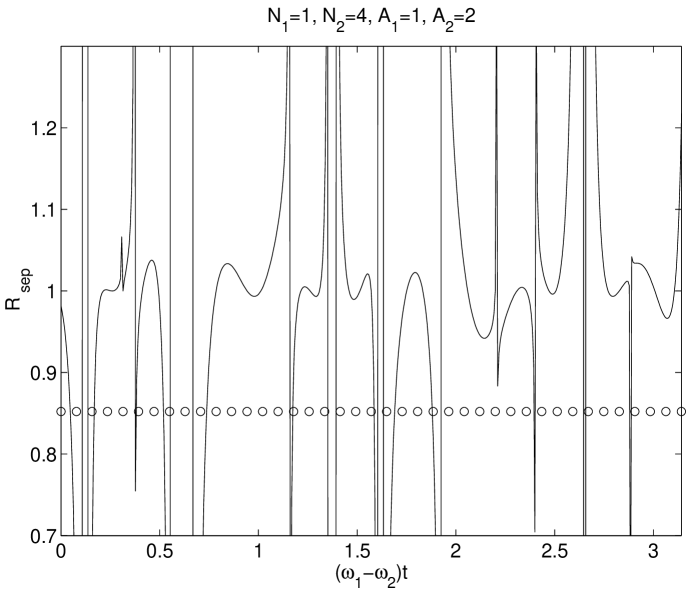
Figure 2: $R_{\rm sep}$ against $(\omega_{1}-\omega_{2})t$ for the number state of Eq. (12) with $N_{1}=1,N_{2}=4$ (line of circles), and the coherent state of Eq. (25) with $A_{1}=1,A_{2}=2$ (solid line). The photon frequencies are $\omega_{1}=1.2\times 10^{-4}$ and $\omega_{2}=10^{-4}$, in units where $k_{B}=\hbar=c=1$.

For microwaves in the entangled state of Eq. (26) the reduced density matrices are

$$\rho_{\rm ent,A}=\rho_{\rm ent,B}={\cal N}^{2}(|A_{1}\rangle\langle A_{1}|+|A_{2}\rangle\langle A_{2}|+\tau|A_{1}\rangle\langle A_{2}|+\tau^{*}|A_{2}\rangle\langle A_{1}|),$$ (30)

where $\tau=\langle A_{1}|A_{2}\rangle=\exp(-|A_{1}|^{2}/2-|A_{2}|^{2}/2+A_{1}^{*}A_{2})$.

The current in A is

$$\langle\hat{I}_{\rm A}\rangle_{\rm ent}=2{\cal N}^{2}\langle\hat{I}_{\rm A}\rangle_{\rm sep}+{\cal N}^{2}EF_{1}\exp\left(-\frac{q^{2}}{2}\right)I_{1},$$ (31)

where $E=\exp[-|A_{1}|^{2}-|A_{2}|^{2}+2|A_{1}A_{2}|\cos(\theta_{1}-\theta_{2})]$, and

$$F_{1}=[\exp(q|A_{1}|S_{A,1}-q|A_{2}|S_{A,2})+\exp(-q|A_{1}|S_{A,1}$$ (32)

$$+q|A_{2}|S_{A,2})]\sin(\omega_{A}t+q|A_{1}|C_{A,1}+q|A_{2}|C_{A,2}),$$

with $S_{A,1}=\sin(\omega_{1}t-\theta_{1})$, $S_{A,2}=\sin(\omega_{1}t-\theta_{2})$, $C_{A,1}=\cos(\omega_{1}t-\theta_{1})$, $C_{A,2}=\cos(\omega_{1}t-\theta_{2})$. A similar expression yields the current in B, and we have also calculated numerically the ratio $R_{\rm ent}$.

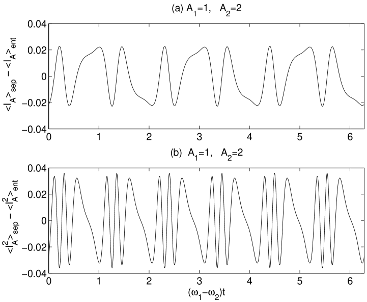
Figure 3: (a) $\langle{\hat{I}}_{\rm A}\rangle_{\rm sep}-\langle{\hat{I}}_{\rm A}\rangle_{\rm ent}$, and (b) $\langle{\hat{I}}_{\rm A}^{2}\rangle_{\rm sep}-\langle{\hat{I}}_{\rm A}^{2}\rangle_{\rm ent}$ against $(\omega_{1}-\omega_{2})t$ for the coherent state $\rho_{\rm sep,A}$ of Eq. (28) and $\rho_{\rm ent,A}$ of Eq. (30) with $A_{1}=1,A_{2}=2$. The photon frequencies are $\omega_{1}=1.2\times 10^{-4}$ and $\omega_{2}=10^{-4}$, in units where $k_{B}=\hbar=c=1$.

3.3 Numerical results

In the numerical results of Figs. 2 and 3 the microwave frequencies are $\omega_{1}=1.2\times 10^{-4},\omega_{2}=10^{-4}$, in units where $k_{B}=\hbar=c=1$. The critical currents are $I_{1}=I_{2}=1$. The other parameters are $\xi=1$, $\omega_{\rm A}=\omega_{1}$, $\omega_{\rm B}=\omega_{2}$, $N_{1}=1$, $N_{2}=4$, and $\theta_{1}=\theta_{2}=0$. For a meaningful comparison between microwaves in number states and microwaves in coherent states, we take them to have the same average number of photons, $|A_{1}|^{2}=N_{1}$ and $|A_{2}|^{2}=N_{2}$.

In Fig. 2 we plot $R_{\rm sep}$ against $(\omega_{1}-\omega_{2})t$ for currents induced by microwaves in the number state of Eq. (12) with $N_{1}=1,N_{2}=4$ (line of circles), and the coherent state of Eq. (25) with $A_{1}=1,A_{2}=2$ (solid line). It is seen that two different separable photon states with the same average number of photons give rise to different correlations between the SQUID currents.

In Fig. 3 we plot (a) $\langle{\hat{I}}_{\rm A}\rangle_{\rm sep}-\langle{\hat{I}}_{\rm A}\rangle_{\rm ent}$, and (b) $\langle{\hat{I}}_{\rm A}^{2}\rangle_{\rm sep}-\langle{\hat{I}}_{\rm A}^{2}\rangle_{\rm ent}$, against $(\omega_{1}-\omega_{2})t$ for microwaves in the coherent state $\rho_{\rm A,sep}$ of Eq. (28) and $\rho_{\rm A,ent}$ of Eq. (30) with $A_{1}=1,A_{2}=2$. In Fig. 3(a) it is seen that the Josephson current in SQUID ring A is different for irradiation with separable and entangled microwaves in coherent states. In Fig. 3(b) it is seen that irradiation with separable and entangled coherent states leads to different second moments of the current, which implies that the quantum statistics of electron pairs tunnelling the Josephson junction of SQUID ring A are different in these two cases.

4 Discussion

We have considered the interaction of two distant SQUID rings A and B with two-mode nonclassical microwaves, which are produced by the same source. The flux, the phase difference and the Josephson currents are operators and their expectation values with the density matrix of the nonclassical microwaves give the physically observed quantities. We have assumed the external field approximation, where the electromagnetic field created by the Josephson currents (back reaction) is neglected and we have calculated various quantities.

It has been shown that the Josephson currents in the two rings are correlated in the sense that $\langle\hat{I}_{\rm A}\hat{I}_{\rm B}\rangle$ is different from $\langle\hat{I}_{\rm A}\rangle\langle\hat{I}_{\rm B}\rangle$ (for non-factorizable density matrices). We have considered examples where the photons are classically correlated and quantum mechanically correlated; and we have shown that the non-diagonal terms in the latter case affect the Josephson currents. Further work in this direction could be the formulation of Bell-type inequalities for the Josephson currents, which are obeyed in the case of separable microwaves and violated in the case of entangled microwaves.

References

[1]
N. Byers and C.N. Yang, Phys. Rev. Lett. 7, 46 (1961); F. Bloch,
Phys. Rev. B 2, 109 (1970); A. Barone and G. Paterno, Physics
and Applications of the Josephson Effect (Wiley, New York, 1982); M. Tinkham,
Introduction to Superconductivity (McGraw-Hill, New York, 1996).
[2]
Y. Makhlin, G. Schön, and A. Shnirman, Rev. Mod. Phys. 73, 357
(2001); M.A. Kastner, ibid.64, 849 (1992); G. Schön and
A.D. Zaikin, Phys. Rep. 198, 237 (1990).
[3]
I. Chiorescu, Y. Nakamura, C. Harmans, and J. Mooij, Science 299,
1869 (2003); Y. Nakamura, Y.A. Pashkin, and J.S. Tsai, Nature 398,
786 (1999); C.H. van der Wal, et al., Science 290, 773 (2000).
[4]
R. Loudon and P.L. Knight, J. Mod. Optics 34, 709 (1987); R. Loudon,
The Quantum Theory of Light (Oxford Univ. Press, Oxford, 2000); D.F.
Walls and G. Milburn, Quantum Optics (Springer, Berlin, 1994).
[5]
A. Vourdas, Phys. Rev. B 49, 12 040 (1994); Z. Phys. B 100,
455 (1996); A. Vourdas and T.P. Spiller, ibid.102, 43 (1997);
A.A. Odintsov and A. Vourdas, Europhys. Lett. 34, 385 (1996).
[6]
L.M. Kuang, Y. Wang, and M.L. Ge, Phys. Rev. B 53, 11 764 (1996); J.
Zou, B. Shao, and X.S. Xing, ibid.56, 14 116 (1997); Phys.
Lett. A 231, 123 (1997); Z. Phys. B 104, 439 (1997); M.J.
Everitt, et al., Phys. Rev. B 63, 144 530 (2001); W. Al-Saidi
and D. Stroud, ibid.65, 014512 (2002).
[7]
D.I. Tsomokos, C.C. Chong, and A. Vourdas, Phys. Rev. A 69, 013810
(2004); Phys. Rev. B, to appear (2004).
[8]
R.F. Werner, Phys. Rev. A 40, 4277 (1989); R. Horodecki and M.
Horodecki, ibid.54, 1838 (1996); A. Peres, Phys. Rev. Lett. 77, 1413 (1996); V. Vedral et al., ibid.78, 2275 (1997);
V. Vedral, Rev. Mod. Phys. 74, 197 (2002).
[9]
See, for example, S. Chountasis and A. Vourdas, Phys. Rev. A 58, 848
(1998) and references therein.