Entangling flux qubits with a bipolar dynamic inductance

Abstract

We propose a scheme to implement variable coupling between two flux qubits using the screening current response of a dc Superconducting QUantum Interference Device (SQUID). The coupling strength is adjusted by the current bias applied to the SQUID and can be varied continuously from positive to negative values, allowing cancellation of the direct mutual inductance between the qubits. We show that this variable coupling scheme permits efficient realization of universal quantum logic. The same SQUID can be used to determine the flux states of the qubits.

A rich variety of quantum bits (qubits) is being explored for possible implementation in a future quantum computer roadmap (2004). Of these, solid state qubits are attractive because of their inherent scalability using well established microfabrication techniques. A subset of these qubits is superconducting, and includes devices based on charge Nakamura et al. (1999); Vion et al. (2002), magnetic flux Orlando et al. (1999); Friedman et al. (2000); van der Wal et al. (2000), and the phase difference Martinis et al. (2002) across a Josephson junction. To implement a quantum algorithm, one must be able to entangle multiple qubits, so that an interaction term is required in the Hamiltonian describing a two qubit system. For two superconducting flux qubits, the natural interaction is between the magnetic fluxes. Placing the two qubits in proximity provides a permanent coupling through their mutual inductance Majer et al. (2003). Pulse sequences for generating entanglement have been derived for several superconducting qubits with fixed interaction energies Yamamoto et al. (2003); Strauch et al. (2003). However, entangling operations can be much more efficient if the interaction can be varied and, ideally, turned off during parts of the manipulation. A variable coupling scheme for charge-based superconducting qubits with a bipolar interaction has been suggested recently Averin and Bruder (2003). For flux qubits, while switchable couplings have been proposed previously Mooij et al. (1999); Clarke et al. (2002), these approaches do not enable one to turn off the coupling entirely and require separate coupling and flux readout devices.

In this Letter, we propose a new coupling scheme for flux qubits in which the interaction is adjusted by changing a relatively small current. For suitable device parameters the sign of the coupling can also be changed, thus making it possible to null out the direct interaction between the flux qubits. Furthermore, the same device can be used both to vary the coupling and to read out the flux states of the qubits. We show explicitly how this variable qubit coupling can be combined with microwave pulses to perform the quantum Controlled-NOT (CNOT) logic gate. Using microwave pulses also for arbitrary single-qubit operations, this scheme provides all the necessary ingredients for implementation of scalable univeral quantum logic.

The coupling is mediated by the circulating current $J$ in a dc Superconducting QUantum Interference Device (SQUID), in the zero voltage state, which is coupled to each of two qubits through an identical mutual inductance $M_{qs}$ [Fig. 1(a)]. A variation in the flux applied to the SQUID, $\Phi_{s}$, changes $J$ [Fig. 1(b)]. The response is governed by the screening parameter $\beta_{L}\equiv 2LI_{0}/\Phi_{0}$ and the bias current $I_{b}$, where $I_{b}<I_{c}(\Phi_{s})$, the critical current for which the SQUID switches out of the zero voltage state at $T=0$ in the absence of quantum tunneling. In flux qubit experiments Chiorescu et al. (2003), the flux state is determined by a dc SQUID to which fast pulses of $I_{b}$ are applied to measure $I_{c}(\Phi_{s},T)$. Thus, existing technology allows $I_{b}$ to be varied rapidly, and a single dc SQUID can be used both to measure the two qubits and to couple them together controllably.

Figure 1: (a) SQUID-based coupling scheme. The admittance Y represents the SQUID bias circuitry. (b) Response of SQUID circulating current $J$ to applied flux $\Phi_{s}$ for $\beta_{L}=0.092$ and $I_{b}/I_{c}(0.45\Phi_{0})=0,0.4,0.6,0.85$ (top to bottom). Lower right inset shows $J(\Phi_{s})$ for same values of $I_{b}$ near $\Phi_{s}=0.45\Phi_{0}$. Upper left inset shows $I_{c}$ versus $\Phi_{s}$.

The flux qubit consists of a superconducting loop interrupted by three Josephson tunnel junctions Mooij et al. (1999); Orlando et al. (1999). With a flux bias near the degeneracy point, $\Phi_{0}/2$, a screening current $I_{q}$ can flow in either direction around the qubit loop. Given the tunnel coupling energy $\delta$ between the different directions of $I_{q}$, the ground and first excited states of the qubit correspond to symmetric and antisymmetric superpositions of these two current states. Thus, the dynamics of qubit $i$ can be approximated by the two-state Hamiltonian

$$\mathcal{H}_{i}=-(\epsilon_{i}^{0}/2)\sigma_{z}^{(i)}-(\delta_{i}/2)\sigma_{x}^{(i)}.$$ (1)

The energy biases $\epsilon_{i}^{0}$ are determined by the flux bias of each qubit relative to $\Phi_{0}/2$. The tunnel frequencies $\delta_{i}/h$ are fixed by the device parameters, and are typically a few GHz. For two flux qubits, arranged so that a flux change in one qubit alters the flux in the other, the coupled-qubit Hamiltonian describing the dynamics in the complex 4-dimensional Hilbert space becomes

$$\mathcal{H}=\mathcal{H}_{1}\otimes I^{(2)}+I^{(1)}\otimes\mathcal{H}_{2}-(K/2)\sigma_{z}^{(1)}\otimes\sigma_{z}^{(2)},$$ (2)

where $I^{(i)}$ is the identity matrix for qubit $i$ and $K$ characterizes the coupling energy. For $K<0$, the minimum energy configuration corresponds to anti-parallel fluxes. For two flux qubits coupled through a mutual inductance $M_{qq}$, the interaction energy is fixed at $K_{0}=-2M_{qq}\left|I_{q}^{(1)}\right|\left|I_{q}^{(2)}\right|.$

For the configuration of Fig. 1(a), in addition to the direct coupling, $K_{0}$, the qubits interact by changing the current $J$ in the SQUID. The response of $J$ to a flux change depends strongly on $I_{b}$ [Fig. 1(b)]. When $I_{q}^{(2)}$ switches direction, the flux coupled to the SQUID, $\Delta\Phi_{s}^{(2)}$, induces a change $\Delta J$ in the circulating current in the SQUID, and alters the flux coupled from the SQUID to qubit 1. The corresponding coupling is

$$K_{s}=I_{q}^{(1)}\Delta\Phi_{q}^{(1)}=-2M_{qs}^{2}\left|I_{q}^{(1)}\right|\left|I_{q}^{(2)}\right|{\rm Re}\left(\partial J/\partial\Phi_{s}\right)_{I_{b}}.$$ (3)

The transfer function, $\left(\partial J/\partial\Phi_{s}\right)_{I_{b}}$, is related to the dynamic impedance, ${\cal Z}$, of the SQUID via Hilbert and Clarke (1985)

$$\partial J/\partial\Phi_{s}=i\omega/{\cal Z}=1/{\cal L}+i\omega/{\cal R},$$ (4)

where ${\cal R}$ is the dynamic resistance, determined by $Y$ which dominates any loss in the Josephson junctions, and ${\cal L}$ is the dynamic inductance which, in general, differs from the geometrical inductance of the SQUID, $L$.

We evaluate $\left(\partial J/\partial\Phi_{s}\right)_{I_{b}}$ by current conservation, neglecting currents flowing through the junction resistances:

$$I_{b} = I_{y}+2I_{0}\cos\Delta\gamma\sin\bar{\gamma}-2C(\Phi_{0}/2\pi)\ddot{\bar{\gamma}},$$ (5)

$$J = I_{0}\cos\bar{\gamma}\sin\Delta\gamma-C(\Phi_{0}/2\pi)\Delta\ddot{\gamma}.$$ (6)

Here, $I_{y}$ is the current flowing through the admittance $Y(\omega)$ [Fig. 1(a)], and $I_{0}$ and $C$ are the critical current and capacitance of each SQUID junction. The phase variables are related to the phases across each junction, $\gamma_{1}$ and $\gamma_{2}$, as $\Delta\gamma=(\gamma_{1}-\gamma_{2})/2$ and $\bar{\gamma}=(\gamma_{1}+\gamma_{2})/2$. The phases are constrained by $d\Delta\gamma=(\pi/\Phi_{0})(d\Phi_{s}-LdJ).$

The expression for $K_{s}$ in terms of ${\rm Re}\left(\partial J/\partial\Phi_{s}\right)_{I_{b}}$ (Eq. 3) requires the qubit frequencies to be much lower than the characteristic frequencies of the SQUID. This condition is satisfied by our choice of device parameters, and also ensures that the SQUID stays in its ground state during qubit entangling operations. Furthermore, it is a reasonable approximation to take the $\omega=0$ limit of ${\rm Re}\left(\partial J/\partial\Phi_{s}\right)_{I_{b}}$ to calculate $K_{s}$, so that we can solve Eqs. (5) and (6) numerically to obtain the working point; for the moment we assume $Y(0)=0$. For the small deviations determining $K_{s}$, we linearize Eqs. (5) and (6) and solve for the real part of the transfer function in the low-frequency limit:

$${\rm Re}\left(\frac{\partial J}{\partial\Phi_{s}}\right)_{I_{b}}=\frac{1}{2L_{j}}\frac{1-\tan^{2}\Delta\gamma\tan^{2}\bar{\gamma}}{1+\frac{L}{2L_{j}}(1-\tan^{2}\Delta\gamma\tan^{2}\bar{\gamma})}.$$ (7)

Here, we have introduced the Josephson inductance for one junction, $L_{j}=\Phi_{0}/2\pi I_{0}\cos\Delta\gamma\cos\bar{\gamma}$. For $\beta_{L}\gg 1$, Eq. (7) approaches $1/L$, while for $\beta_{L}\ll 1$,

$${\rm Re}\left(\partial J/\partial\Phi_{s}\right)_{I_{b}}=(1/2L_{j})(1-\tan^{2}\Delta\gamma\tan^{2}\bar{\gamma}).$$ (8)

We see that ${\rm Re}\left(\partial J/\partial\Phi_{s}\right)_{I_{b}}$ becomes negative for sufficiently high values of $I_{b}$ and $\Phi_{s}$, which increase $\bar{\gamma}$ and $\Delta\gamma$.

We choose the experimentally-accessible SQUID parameters $L=200$ pH, $C=5$ fF, and $I_{0}=0.48$ $\mu$A, for which $\beta_{L}=0.092$. The qubits are characterized by $I_{q}^{(1)}=I_{q}^{(2)}=0.46$ $\mu$A, $M_{qs}=33$ pH, and $M_{qq}=0.25$ pH, yielding $K_{0}/h=-0.16$ GHz. Choosing $\Phi_{s}=0.45\Phi_{0}$, Eqs. (3) and (7) result in a net coupling strength $K/h=(K_{0}+K_{s})/h$ that is $-0.3$ GHz when $I_{b}=0$, and zero when $I_{b}/I_{c}(0.45\Phi_{0})=0.57$ [Fig. 2(a)]. The change in sign of $K_{s}$ does not occur for all $\beta_{L}$. Figure 2(b) shows the highest achievable value of $K_{s}$ versus $\beta_{L}$. We have adopted the optimal design at $\beta_{L}=0.092$.

Figure 2: (a) Variation of $K$ with $I_{b}$ for $\Phi_{s}=0.45\Phi_{0}$ and device parameters described in text. (b) Highest achievable value of $K_{s}$ versus $\beta_{L}$ evaluated at $I_{b}=0.85I_{c}(0.45\Phi_{0})$; $I_{0}$ (and hence $\beta_{L}$) is varied for $L=200$ pH.

We also need to consider crosstalk between the coupling and single-qubit terms in the Hamiltonian. When the coupling is switched, in addition to $\partial J/\partial\Phi_{s}$ being altered, $J$ also changes, thus shifting the flux biases of the qubits. The calculated change in $J$ as the coupler is switched from $I_{b}=0$ to $I_{b}/I_{c}(0.45\Phi_{0})=0.57$ produces a change in the flux in each qubit corresponding to an energy shift $\delta\epsilon_{1}/h=\delta\epsilon_{2}/h=1.64$ GHz. In addition, when the qubits are driven by microwaves to produce single-qubit rotations, the microwave flux may also couple to $\Phi_{s}$. As a result, $K$ is weakly modulated when the coupling would nominally be turned off. A typical microwave drive $\tilde{\epsilon}_{i}(t)/h$ of amplitude 1 GHz results in a variation of about $\pm 14$ MHz about $K=0$.

When the bias current is increased to switch off the coupling, the SQUID symmetry is broken and the qubits are coupled to the noise generated by the admittance $Y$. We estimate the decoherence due to this process by calculating the environmental spectral density ${\cal J}(\omega)$ in the spin-boson model Wilhelm et al. (2003). We obtain ${\cal J}(\omega)$ from the classical equation of motion for the qubit flux with the dissipation from $Y$ coupled to either qubit through $J$:

$$\mathcal{J}(\omega)=\left(I_{q}^{2}M_{qs}^{2}/h\right){\rm Im}\left(\partial J/\partial\Phi_{s}\right)_{I_{b}}.$$ (9)

To calculate ${\cal J}(\omega)$, we linearize Eqs. (5) and (6) around the equilibrium point to obtain

$$d\bar{\gamma}=\frac{2\tan\bar{\gamma}\tan\Delta\gamma}{L_{j}}\frac{1}{2/L_{j}-2\omega^{2}C+i\omega Y}d\Delta\gamma.$$ (10)

For the case $Y^{-1}=R$, following the path to the static transfer function Eq. (7) and taking the imaginary part in the low-$\beta_{L}$ limit, we obtain ${\rm Im}(\partial J/\partial\Phi_{s})_{I_{b}}=-\omega/{\cal R}=(\omega/4R)\tan^{2}\Delta\gamma\tan^{2}\bar{\gamma}$. Thus ${\cal J}(\omega)=\alpha\omega$, where $\alpha=(M_{qs}^{2}I_{q}^{2}/4hR)\tan^{2}\Delta\gamma\tan^{2}\bar{\gamma}$, and $\alpha(I_{b}=0)=0$. As $I_{b}$ is increased to change the coupling strength, $\alpha$ increases monotonically. For the parameters described above and for $R=2.4$ k$\Omega$, when the net coupling is zero [$I_{b}/I_{c}(0.45\Phi_{0})=0.57$, Fig. 2(a)] we find $\alpha=8\times 10^{-5}$, corresponding to a qubit dephasing time of about $500$ ns, one order of magnitude larger than values currently measured in flux qubits Chiorescu et al. (2003).

We now show that this configuration implements universal quantum logic efficiently. Any $n$-qubit quantum operation can be decomposed into combinations of two-qubit entangling gates, for example, CNOT, and single-qubit gates  Barenco et al. (1995). Single-qubit gates generate local unitary transformations in the complex 2-dimensional subspace for the corresponding individual qubit, while the two-qubit gates correspond to unitary transformations in the 4-dimensional Hilbert space. Two-qubit gates which cannot be decomposed into a product of single-qubit gates are said to be nonlocal, and may lead to entanglement between the two qubits Zhang et al. (2003). Since we can adjust the qubit coupling $K$ to zero, we can readily implement single-qubit gates with microwave pulses as described below.

To implement the nonlocal two-qubit CNOT gate, we use the concept of local equivalence: the two-qubit gates $U_{1}$ and $U_{2}$ are locally equivalent if $U_{1}=k_{1}U_{2}k_{2}$, where $k_{1}$ and $k_{2}$ are local two-qubit gates which are combinations of single-qubit gates applied simultaneously. These unitary transformations on the two single-qubit subspaces transform the gate $U_{2}$ into $U_{1}$. The local gate which precedes $U_{2}$, $k_{2}$, is given by $k_{21}\otimes k_{22}$, where $k_{21(22)}$ is a single-qubit gate for qubit $1(2)$, while the local gate which follows $U_{2}$, $k_{1}$, is $k_{11}\otimes k_{12}$, where $k_{11(12)}$ is a single-qubit gate for qubit $1(2)$ Makhlin (2002). Our strategy is to find efficient implementation of a nonlocal quantum gate $U_{2}$ that differs only by local gates, $k_{1}$ and $k_{2}$, from CNOT, using the methods in Zhang et al. (2003), and then to add those local operations required to achieve a CNOT gate in the computational basis, in which the SQUID measures the projection of each qubit state vector onto the z-axis.

The local equivalence classes of two-qubit operations have been shown Zhang et al. (2003) to be in one-to-one correspondence with points in a tetrahedron, the Weyl chamber. In this geometric representation, any two-qubit operation is associated with the point $[c_{1},c_{2},c_{3}]$, where CNOT corresponds to $[\pi/2,0,0]$. Furthermore, the nonlocal two-qubit gates generated by a Hamiltonian acting for time $t$ can be mapped to a trajectory in this space Zhang et al. (2003). If $K$ is increased instantaneously to a constant value, the trajectory generated by Eq. (2) is well described by the following periodic curve

$$[c_{1},c_{2},c_{3}]=\left[Kvt/\hbar,p\left|\sin\omega t\right|,p\left|\sin\omega t\right|\right].$$ (11)

Here, $p$ is a function of the system parameters, $v=\epsilon_{1}^{0}\epsilon_{2}^{0}/\Delta E_{1}\Delta E_{2}$, and $\omega=(\Delta E_{1}-\Delta E_{2})/2\hbar$, where $\Delta E_{i}=[(\epsilon_{i}^{0})^{2}+\delta_{i}^{2}]^{1/2}$ is the single-qubit energy level splitting. Independently of $p$, this trajectory reaches $[\pi/2,0,0]$ in a time $t_{K}=n\pi/\omega$ when the coupling strength is tuned to $K=\hbar\omega/2nv$, with $n$ a nonzero integer.

While this analytic solution contains the essential physics, it is an approximation and does not include vital experimental features, in particular, crosstalk and the finite rise time of the bias current pulse. To improve the accuracy, we perform a numerical optimization using Eq. (11) as a starting point, then add these corrections. We use tunnel frequencies $\delta_{1}/h=5$ GHz and $\delta_{2}/h=3$ GHz, and include the shifts of the single-qubit energy biases due to the crosstalk with $K_{s}$ in Eq. (11) by adding a shift $\delta\epsilon_{i}$ proportional to $K$. We account for the rise and fall times of the current pulse by using pulse edges with $90\%$ widths of $0.5$ ns [see $K(t)$ in Fig. 3]. We numerically optimize the variable parameters to minimize the Euclidean distance between the actual achieved gate and the desired Weyl chamber target CNOT gate. We find $K/h=-0.30$ GHz, $\epsilon_{1}^{0}/h=8.06$ GHz, $\epsilon_{2}^{0}/h=2.03$ GHz, and $t_{K}=8.74$ ns; $t_{K}$ is the time during which the qubit coupling is turned on.

As outlined above, to achieve a true CNOT gate we still have to determine the pulse sequences which implement the requisite local gates that take this Weyl chamber target $U_{2}$ to CNOT in the computational basis. Local gates may be implemented by applying microwave radiation, $\tilde{\epsilon}_{i}(t)$, which couples to $\sigma_{z}^{(i)}$, and is at or near resonance with the single-qubit energy level splitting $\Delta E_{i}$. We note that the single-qubit Hamiltonian of Eq. (1) driven by a resonant oscillating microwave field does not permit one to use standard NMR pulses, since the static and oscillating fields are not perpendicular, but rather are canted by an angle $\tan^{-1}(\delta_{i}/\epsilon_{i}^{0})$. To simplify the pulse sequence, we keep $\epsilon_{1,2}^{0}$ constant at the values used for the non-local gate generation. This imposes an additional constraint on the local gates: to generate a local two-qubit gate $k_{1}=k_{11}\otimes k_{12}$, the two single-qubit gates $k_{11}$ and $k_{12}$ must be simultaneous and of equal duration. We satisfy this constraint by making the microwave pulse addressing one qubit resonant and that addressing the other slightly off-resonance. Using this offset and the relative amplitude and phase of the two microwave pulses as variables, we can achieve two different single-qubit gates simultaneously, leading to our required local two-qubit gate.

The resulting pulse sequences for $K$ and $\tilde{\epsilon}_{1,2}$ are shown in Fig. 3. The gate has a maximum deviation from CNOT in the computational basis of $1.6\%$ in any matrix element. This error arises predominantly from the cross-coupling of the microwave signals for the two qubits and the weak modulation of the $K=0$ state of the coupler during the single-qubit microwave manipulations. While small, this error could be reduced further by performing the numerical optimization with higher precision or by coupling the microwave flux selectively to each of the qubits and not to the SQUID. The total elapsed time of $29.35$ ns is comparable to measured dephasing times in a single flux qubit Chiorescu et al. (2003).

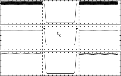
Figure 3: Pulse sequence for implementing CNOT gate. Energy scales in GHz. Total single-qubit energy bias $\epsilon_{i}(t)=\epsilon_{i}^{0}+\tilde{\epsilon}_{i}(t)+\delta\epsilon_{i}(t)$, where microwave pulses $\tilde{\epsilon}_{1,2}(t)$ produce single-qubit rotations in the decoupled configuration; crosstalk modulation of $K(t)$ is shown (see text). The bias current is pulsed to turn on the interaction in the central region.

Figure 4: Chain of flux qubits with intervening dc SQUIDs arranged to provide both variable nearest neighbor coupling and qubit readout.

In summary, we have shown that the inverse dynamic inductance of a dc SQUID with low $\beta_{L}$ in the zero-voltage state can be varied by pulsing the bias current. This technique provides a variable-strength interaction $K_{s}$ between flux qubits coupled to the SQUID, and enables cancellation of the direct mutual inductive coupling $K_{0}$ between the qubits so that the net coupling $K$ can be switched from a substantial value to zero. By steering a nonlocal gate trajectory and combining it with local gates composed of simultaneous single-qubit rotations driven by resonant and off-resonant microwave pulses, we have shown that a simple pulse sequence containing a single switching of the flux coupling for fixed static flux biases results in a CNOT gate and full entanglement of two flux qubits on a timescale comparable to measured decoherence times for flux qubits. Furthermore, the same SQUID can be used to determine the flux state of the qubits. This approach should be readily scalable to larger numbers of qubits, as, for example, in Fig. 4.

This work was supported by the Air Force Office of Scientific Research under Grant F49-620-02-1-0295, the Army Research Office under Grants DAAD-19-02-1-0187 and P-43385-PH-QC, and the National Science Foundation under Grant EIA-020-5641. FKW acknowledges travel support from DFG within SFB 631.

References

- roadmap (2004) A Quantum Information Science and Technology Roadmap, Version 2.0, April 2, 2004, LA-UR-04-1778, http://qist.lanl.gov.
- Nakamura et al. (1999) Y. Nakamura et al., Nature 398, 786 (1999).
- Vion et al. (2002) D. Vion et al., Science 296, 286 (2002).
- Orlando et al. (1999) T. P. Orlando et al., Phys. Rev. B 60, 15398 (1999).
- Friedman et al. (2000) J. R. Friedman et al., Nature 46, 43 (2000).
- van der Wal et al. (2000) C. H. van der Wal et al., Science 290, 773 (2000).
- Martinis et al. (2002) J. M. Martinis et al., Phys. Rev. Lett. 89, 117901 (2002).
- Majer et al. (2003) J. Majer et al., cond-mat/0308192.
- Yamamoto et al. (2003) T. Yamamoto et al., Nature 425, 941 (2003).
- Strauch et al. (2003) F. Strauch et al., Phys. Rev. Lett. 91, 167005 (2003).
- Averin and Bruder (2003) D. V. Averin and C. Bruder, Phys. Rev. Lett. 91, 057003 (2003).
- Mooij et al. (1999) J. Mooij et al., Science 285, 1036 (1999).
- Clarke et al. (2002) J. Clarke et al., Physica Scripta T102, 173 (2002).
- Zhang et al. (2003) J. Zhang et al., Phys. Rev. A 67, 042313 (2003).
- Hilbert and Clarke (1985) C. Hilbert and J. Clarke, J. Low Temp. Phys. 61, 237 (1985).
- Wilhelm et al. (2003) F. K. Wilhelm et al., Adv. Solid State Phys. 43, 763 (2003).
- Chiorescu et al. (2003) I. Chiorescu et al., Science 299, 1869 (2003).
- Barenco et al. (1995) A. Barenco et al., Phys. Rev. A 52, 3457 (1995).
- Makhlin (2002) Y. Makhlin, Quant. Inf. Processing 1, 243 (2002).