Soliton Atom Laser with Quantum State Transfer Property

Xiong-Jun Liu^a,b, Hui Jing^c and Mo-Lin Ge^b

a. Department of Physics, National University of Singapore, 10 Kent Ridge Crescent, Singapore 119260, Singapore

b. Theoretical Physics Division, Nankai Institute of Mathematics,Nankai University, Tianjin 300071, P.R.China

c. State Key Laboratory of Magnetic Resonance and Atomic and Molecular Physics,

Wuhan Institute of Physics and Mathematics, CAS, Wuhan 430071, P. R. China

Abstract

We propose a scheme to obtain soliton atom laser with nonclassical atoms based on quantum state transfer process from light to matter waves in nonlinear case, which may find novel applications in, e.g., an atom interferometer. The dynamics of the atomic gray solitons and the accompanied frequency chirp effect are discussed.

PACS numbers: 03.75.-b, 42.50.Gy, 03.65.Ta, 03.67.-a

Since the first pulsed atom laser was created in 1997 through RF output coupling of a trapped atomic Bose-Einstein condensate [1], there have been many interests in preparing a continuous atom laser and exploring its potential applications in, e.g., gravity measurements through atom interferometry [2]. Although a sub-quantum-noise atom laser is expected to be crucial to improve the interferometer sensitivities, the difficulties for the atomic beam to propagate over a long distance heavily restrict its actual performance [3]. Some time ago Drummond et al. proposed to use mode-locking technique to stabilize the atom laser based on the generation of a dark soliton in a ring-shaped condensate [4]. Other related works are the atomic soliton formation and its stationary transmission in a travelling optical laser beam [5] or a waveguide [6] for a dense atomic flow. While optical techniques are by now well developed to make and control a soliton laser [7] (even using an interferometer [8]), less progress has been made for ultracold atoms. We here propose a novel scheme to obtain a soliton atom laser with nonclassical characteristic via the versatile quantum state transfer technique [10, 11, 12, 13].

Recently, by manipulating two external lights for an ensemble of $3$-level $\Lambda$ type atoms, the physical mechanism of Electromagnetically Induced Transparency (EIT) [14] has attracted much attention in both experimental and theoretical aspects [10, 11, 12], especially after the dark-states polaritons (DSPs) theory [13] was proposed and thereby the rapid developments of quantum memory technique, i.e., transferring the quantum states of photon wave-packet to collective Raman excitations in a loss-free and reversible manner. By extending the transfer technique to matter waves, a wonderful scheme was proposed to make a continuous atomic beam with nonclassical or entangled states [15], which was later confirmed also for double-$\Lambda$ 4-level atoms [16].

Nonetheless, in these pioneering works the role of nonlinear atomic interactions in the quantum state transfer process was neglected [15, 16]. In this paper, by studying the quantum states transfer technique from photons to atomic beam in the nonlinear case, we propose a scheme to obtain a soliton atom laser with nonclassical atoms. The dynamics of present gray-solitons is shown to be free of the atomic frequency chirp effect occurring in state transfer process. Essentially being different from output couplings of atomic solitons formed in a trapped condensate [4, 17, 18, 19], this scheme should be realizable in the next generation of experiments.

The development herein is outlined as follows. Firstly, we study the role of nonlinear atomic interactions in the transfer process of quantum states from probe field to matter waves in adiabatic condition. For present purpose, the collisions between the initial-state atoms ($\Phi_{1}$) are omitted by, e.g., applying the recently developed novel technique of magnetic-field-induced Feshbach resonance [9], while nonlinear interaction between the generated atoms ($\Phi_{2}$) is well considered. The quantum transfer character is still confirmed except for an additional phase leading to the frequency chirp effect [20]. Secondly, we focus on the formation and dynamics of atomic solitons in the output beam, including the speed, the free-chirp property, etc. Finally, we discuss the possibilities of further manipulations of soliton atom laser.

Turning to the situation of Fig.1. The situation we consider is a beam of three-level $\Lambda$ type atoms moving in the $z$ direction interact with a quantum probe and a control Stokes field and the former field is taken to be much weaker than the later. Atoms in different internal states are described by three bosonic fields $\hat{\Psi}_{\mu}(z,t)(\mu=1,2,3)$. The Stokes field coupling the transition from meta-stable state $|2\rangle$ to excited one $|3\rangle$ can be described by the Rabi-frequencies $\Omega_{s}=\Omega_{0}(z)e^{-i\omega_{s}(t-z/c^{\prime})}$ with $\Omega_{0}$ being taken as real, and $c^{\prime}$ denoting the phase velocities projected onto the $z$ axis. The quantized probe field coupling the transition from ground state $|1\rangle$ to $|3\rangle$ are characterized by the dimensionless positive frequency component $\hat{E}^{(+)}_{p}(z,t)=\hat{\cal E}(z,t)e^{-i\omega_{p}(t-z/c)}$. We can introduce the slowly-varying amplitudes $\hat{\Psi}_{1}=\hat{\Phi}_{1}e^{i(k_{0}z-\omega_{0}t)}$, $\hat{\Psi}_{2}=\hat{\Phi}_{2}e^{i[(k_{0}+k_{p}-k_{s})z-(\omega_{0}+\omega_{p}-\omega_{s})t]}$ and $\hat{\Psi}_{3}=\hat{\Phi}_{3}e^{i[(k_{0}+k_{p})z-(\omega_{0}+\omega_{p})t]}$, where $\hbar\omega_{0}=\hbar^{2}k^{2}_{0}/2m$ is the corresponding kinetic energy in the average velocity, $k_{p}$ and $k_{s}$ are respectively the vector projections of the probe and Stokes fields to the $z$ axis. The atoms have a narrow velocity distribution around $v_{0}=\hbar{k_{0}}/m$ with $k_{0}\gg|k_{p}-k_{s}|$, and all fields are assumed to be in resonance for the central velocity class. The Hamiltonian of the total system is $H=H_{0}+H_{coll}+H_{I}$, where (under the $s$-wave approximation)

$$H_{0} = \sum_{j=1,2,3}\int dz\hat{\Psi}_{j}^{{\dagger}}(-\frac{\hbar^{2}}{2m}\frac{\partial^{2}}{\partial z^{2}}+\hbar V_{j})\hat{\Psi}_{j},$$ (1)

$$H_{1} = \sum_{i,j=1,2}\hbar U_{ij}\int dz\hat{\Psi}^{{\dagger}}_{i}\hat{\Psi}^{{\dagger}}_{j}\hat{\Psi}_{i}\hat{\Psi}_{j},$$ (2)

$$H_{I} = -\int dz\hat{\Psi}^{{\dagger}}_{3}[\hbar g\hat{E}(z,t)]\hat{\Psi}_{1}-\int dz\hat{\Psi}^{{\dagger}}_{3}[\hbar\Omega_{s}(z,t)]\hat{\Psi}_{2}+h.c.$$ (3)

are the free atomic part, atomic collision part and atom-field interaction part, respectively. The Heisenberg equations for the bosonic field operators are governed by [21]

$$i\hbar\frac{\partial\hat{\Psi}_{1}}{\partial t}=[-\frac{\hbar^{2}}{2m}\frac{\partial^{2}}{\partial z^{2}}+V_{1}(z)+U_{11}\hat{\Psi}_{1}^{{\dagger}}\hat{\Psi}_{1}+U_{12}\hat{\Psi}_{2}^{{\dagger}}\hat{\Psi}_{2}]\hat{\Psi}_{1}+\hbar g\hat{E}_{p}^{{\dagger}}\hat{\Psi}_{3}$$ (4)

$$i\hbar\frac{\partial\hat{\Psi}_{2}}{\partial t}=[(\epsilon_{12}-\frac{\hbar^{2}}{2m}\frac{\partial^{2}}{\partial z^{2}})+V_{2}(z)+U_{21}\hat{\Psi}_{1}^{{\dagger}}\hat{\Psi}_{1}+U_{22}\hat{\Psi}_{2}^{{\dagger}}\hat{\Psi}_{2}]\hat{\Psi}_{2}+\hbar\Omega_{s}^{*}\hat{\Psi}_{3}$$ (5)

$$i\hbar\frac{\partial\hat{\Psi}_{3}}{\partial t}=[(\epsilon_{13}-\frac{\hbar^{2}}{2m}\frac{\partial^{2}}{\partial z^{2}})+i\hbar\gamma+V_{3}(z)]\hat{\Psi}_{3}+\hbar g\hat{E}_{p}\hat{\Psi}_{1}+\hbar\Omega_{s}\hat{\Psi}_{2}$$ (6)

where $V_{i}(z)(i=1,2,3)$ are the longitudinal external effective potentials of which $V_{1}(z)$, similar to the previous works, will be chosen as $V_{1}(z)=0$ in the following derivation [15, 16, 22], $g$ is the atom-field coupling constant between the states $|1\!\!>$ and $|3\!\!>$ [13], $\epsilon_{13}=\hbar(\omega_{31}-\omega_{p})$ and $\epsilon_{12}=\hbar(\omega_{21}-\omega_{p}-\omega_{s})$ are energies of the single and two-photon detunings. $\gamma$ denotes the loss rate out of the excited state and the scattering length $a_{ij}$ characterizes the atom-atom interactions via $U_{ij}=4\pi\hbar^{2}a_{ij}/m$. Since almost no atoms occupy the excited state $|3\!\!>$ in the dark-state condition fulfilled in the EIT technique, the collisions between $|3\!\!>$ and lower states can be safely omitted. The propagation equation of the probe field reads: $(\frac{\partial}{\partial{t}}+c\frac{\partial}{\partial{z}})\hat{\cal E}(z,t)=-ig\hat{\Psi}^{{\dagger}}_{1}\hat{\Psi}_{3}e^{-i(k_{p}z-\omega_{p}t)}.$ And the depletion of the strong classical Stokes field is neglected.

We can study the adiabatic situation by ignoring the two photon-detuning and the decaying of excited states. From Eq.(6), we obtain that $\hat{\Psi}_{2}=-\frac{g\hat{E}(z,t)}{\Omega_{s}(z,t)}\hat{\Psi}_{1}=-\frac{g\hat{\cal E}(z,t)}{\Omega_{0}(z)}\hat{\Psi}_{1}e^{i[(k_{s}-k_{p})z-(\omega_{s}-\omega_{p})t]}$. Consider a stationary input of atoms in state $|1\!\!>$ and in the limit of weak probe field, we have [15, 16] $\langle\hat{\Psi}_{2}^{{\dagger}}\hat{\Psi}_{2}\rangle\ll\langle\hat{\Psi}_{1}^{{\dagger}}\hat{\Psi}_{1}\rangle$ and then ignore the depletion of the ground-state atoms and the nonlinear term involving $\hat{\Psi}_{2}$ in Eq.(4). Furthermore, we may choose a zero-value scattering length $a_{11}$ through the Feshbach resonance technique [9]. Hence the depletion of atoms in state $|1\rangle$ and all the nonlinear terms in Eq.(4) can be ignored and the solution can be written as $\hat{\Psi}_{1}(z,t)\approx\langle\hat{\Psi}_{1}\rangle=ne^{i(k_{0}z-\omega_{0}t)}$ [15], where $n$ is the constant total density of atoms. The $\hat{\Psi}_{3}$-field reads: $\hat{\Psi}_{3}(z,t)=-\frac{1}{\hbar\Omega_{s}}[\frac{\hbar^{2}}{2m}\frac{\partial^{2}}{\partial z^{2}}+i\hbar\frac{\partial}{\partial t}-V_{2}(z)-U_{21}n-U_{22}\hat{\Psi}_{2}^{{\dagger}}\hat{\Psi}_{2}^{2}]\frac{g\hat{E}(z,t)}{\Omega_{s}}\Psi_{1}$. Now we reach the following equation of motion for the radiation field:

$$i\hbar\bigl{[}(1+\frac{g^{2}n}{\Omega^{2}_{0}(z)})\frac{\partial}{\partial{t}}+c(1+\frac{g^{2}n}{\Omega^{2}_{0}(z)}\frac{v}{c}-i\frac{g^{2}n}{\Omega^{2}_{0}(z)}\frac{v}{c}\frac{\partial_{z}\ln\Omega_{0}}{k})\frac{\partial}{\partial{z}}\bigl{]}\hat{\cal E}(z,t)$$

$$-\bigr{(}A(z)+B(z)\hat{\cal E}^{{\dagger}}\hat{\cal E}\bigr{)}\hat{\cal E}(z,t)=i\hbar\frac{g^{2}n}{\Omega^{2}_{0}(z)}v(\frac{\partial}{\partial{z}}\ln\Omega_{0}(z))\hat{\cal E}(z,t).$$ (7)

Here we neglect the second derivative of slowly-varying amplitude $\hat{\cal E}$ and assume the sufficiently slowly spatial variations of $\Omega_{0}$ [15, 16]. $A(z)=\frac{g^{2}n}{\Omega_{0}^{2}}\bigl{[}(V_{2}(z)+nU_{21})+\frac{v_{0}^{2}}{2k_{0}^{2}}\bigl{(}(\frac{\partial\ln\Omega_{0}}{\partial z})^{2}-\frac{\partial^{2}\ln\Omega_{0}}{\partial z^{2}}\bigl{)}\bigl{]}$, $B(z)=U_{22}\frac{g^{4}n^{2}}{\Omega^{4}_{0}(z)}$, $k=k_{0}+k_{p}-k_{c}$ and $v=v_{0}+v_{r}$ with $v_{r}=\hbar(k_{p}-k_{c})/m$ being the recoil velocity for $|1>\rightarrow|3>$ transition in $z$ direction. Although the probe field is weak (and then the generated atomic beam $\Phi_{2}$ is also weak, see the following context), the ultra-slow light case ($\frac{g^{2}n}{\Omega^{2}_{0}}\gg 1$) can greatly enhance the nonlinear interaction. Since $k_{0}$ is a very large factor $(k_{0}\gg|k_{p}-k_{c}|)$, we have $|\partial_{z}\ln\Omega_{0}/k|\ll 1$. For this the corresponding parts in above equation can safely be neglected. By introducing the mixing angle $\theta(z)$ according to $\tan^{2}\theta(z)\equiv\frac{g^{2}n}{\Omega_{0}^{2}}\frac{v}{c}$, we can obtain the final solution

$$\hat{\cal E}(z,t)=\frac{\cos\theta(z)}{\cos\theta(0)}\hat{\cal E}\bigl{(}0,T\bigl{)}\exp\bigl{(}-i\hat{\cal E}^{{\dagger}}(0,T)\hat{\cal E}(0,T)\int_{0}^{z}|\frac{\cos\theta(\xi)}{\cos\theta(0)}|^{2}B^{\prime}(\xi)d\xi-i\int_{0}^{z}A^{\prime}(\xi)d\xi\bigl{)},$$ (8)

where $T=t-\tau(z)=t-\int^{z}_{0}{d\xi V^{-1}_{g}(\xi)}$ is the time scale in rest frame, the group velocity $V_{g}=c(1+\frac{g^{2}n}{\Omega^{2}}\frac{v}{c})/(1+\frac{g^{2}n}{\Omega^{2}})$ approaches $v$ for $\Omega(z)\rightarrow 0$. $A^{\prime}(\xi)=A(\xi)/(1+\frac{g^{2}n}{\Omega_{0}^{2}(\xi)})\hbar$ and $B^{\prime}(\xi)=B(\xi)/(1+\frac{g^{2}n}{\Omega_{0}^{2}(\xi)})\hbar$. In particular, by assuming $\theta(0)=0$ and $\theta(L)=\pi/2$ at the input and output regions respectively, one clearly sees that the slowly-varying amplitude of the bosonic field $\hat{\Psi}_{2}$ can be written as

$$\hat{\Phi}_{2}(z,t)=\sqrt{\frac{c}{v}}\ \hat{\cal E}\bigr{(}0,t-\tau(z)\bigr{)}\exp\bigr{(}i\Delta\phi(z,t)\bigr{)},\ \ (z\geq L)$$ (9)

with an additional quantum phase $\Delta\phi(z,t)=\int_{0}^{z}A^{\prime}(\xi)d\xi\bigl{)}+\hat{\cal E}^{{\dagger}}(0,T)\hat{\cal E}(0,T)\int_{0}^{z}|\cos\theta(\xi)|^{2}B^{\prime}(\xi)d\xi$ [15]. The factor $\sqrt{c/v}$ shows that the input light propagate with velocity $c$ while the output atoms with $v$. Obviously, the presence of intrinsic nonlinear atomic interaction leads to a self-phase modification (SPM) in the quantum state transfer process. Due to the time-dependent character of $\Delta\phi$, it indicates an atom laser with frequency chirp $\delta\omega=-\frac{\partial\Delta\phi(z,t)}{\partial T}=-\frac{\partial|{\cal E}(0,T)|^{2}}{\partial T}\int_{0}^{z}|\cos\theta(\xi)|^{2}B^{\prime}(\xi)d\xi$, and $|{\cal E}(0,T)|^{2}=\langle\hat{\cal E}^{{\dagger}}(0,T)\hat{\cal E}(0,T)\rangle$, which may hold the promise to find some actual applications [20].

As a concrete example, let us consider a Gaussian or super Gaussian envelop for the input probe field (see Fig.2(a)) and then obtain the following expression:

$$\delta\omega(T)=\frac{2m}{T_{0}}\int_{0}^{z}|\cos\theta(\xi)|^{2}B^{\prime}(\xi)d\xi\biggr{(}\frac{T}{T_{0}}\biggr{)}^{2m-1}\exp\biggr{[}-\biggr{(}\frac{T}{T_{0}}\biggr{)}^{2m}\biggr{]},\ \ (z\geq L)$$ (10)

where $T_{0}$ is the normalized time scale, $m=1$ and $m=3$ characterizes the Gaussian and super Gaussian pulse, respectively. Using $\Lambda_{0}(z)=\frac{2}{T_{0}}\int_{0}^{z}|\cos\theta(\xi)|^{2}B^{\prime}(\xi)d\xi$ to normalize the frequency, the chirp development is shown in Fig.2(b), from which one can clearly see that the frequency chirp of the output atom laser is significantly dependent on the gradient of the input probe pulse’s front and tail.

Now we proceed to reveal the formation of atomic solitons in the output beam and probe some of its novel properties. For simplicity, our following investigations will adopt the mean-field description (or quasi one-dimension Gross-Pitaevskii equation) [23]. Note that the above quantum state transfer process is clearly independent on this approximation. For this the bosonic field $\hat{\Psi}_{2}(z,t)=\Psi_{2}(z,t)+\hat{\psi}_{2}$, where the condensate wave function $\Psi_{2}$ satisfies the nonlinear Schrödinger equation (NLSE) which supports a gray- (or bright-) soliton solution for a positive (or negative) scattering lenght $a_{22}$ and $\hat{\psi}_{2}$ denotes the quantum fluctuation. Taking into account of the mixing angle $\theta=\pi/2$ in the region $z\geq L$, or the Rabi frequency of the Stokes control field $\Omega_{s}\rightarrow 0$ (meanwhile no transition between the atoms in state $|1\rangle$ and $|2\rangle$), we obtain motion equation for $\Psi_{2}$ in the following form

$$i\hbar\frac{\partial\Psi_{2}}{\partial t}=-\frac{\hbar^{2}}{2m}\frac{\partial^{2}\Psi_{2}}{\partial z^{2}}+V_{2eff}(z)\Psi_{2}+U_{22}|\Psi_{2}|^{2}\Psi_{2}$$ (11)

with an effective potential $V_{2eff}=V_{2}+nU_{21}$. For positive scattering length $a_{22}$ or repulsive atomic interaction, the solution of above equation describing a gray soliton moving in propagating background wave function is [17, 18, 19] $:\Psi_{2}(z,t)=\Psi^{0}_{2}(z,t)\bigr{\{}i\sqrt{1-\eta^{2}}+\eta\tanh\bigl{[}\frac{\eta}{\sqrt{\beta}}(z-z_{0}(t))\bigl{]}\bigr{\}}$, where $\beta=1/(8\pi|\Psi_{2}|^{2}a_{22})^{1/2}$, the external trap $V_{2}(z)$ is chosen such that $V_{2eff}=0$ [15, 16, 22], the background wave function $\Psi^{0}_{2}(z,t)=\Phi_{2}(z,t)\exp\bigl{[}i(kz-\int^{t}_{t_{0}}\lambda dt^{\prime}\bigl{)}+i\varphi_{0}\bigl{]}$ with $\lambda=\frac{k^{2}}{2m}+\frac{U_{22}}{\hbar}|\Phi_{2}|^{2}$ and $\Phi_{2}=\langle\hat{\Phi}_{2}\rangle$, the centra position of the soliton at time $t$ is $z_{0}(t)=\int^{t}_{t_{0}}\mu dt^{\prime}+L$ with $\mu$ the velocity of the solitons, and the parameters $t_{0}$ and $\varphi_{0}$ are respectively the time and phase at position $z=L$. The dimensionless parameter $\eta$ characterizes the ”grayness” with $\eta=1$ corresponding to a ”dark-soliton” with a $100\%$ density depletion. With $\eta\neq 1$, the solitons travel at a sound velocity $\mu=c_{s}(1-\eta^{2})^{1/2}+\hbar k/m$ where $c_{s}=\sqrt{4\pi|\Phi_{2}|^{2}\hbar^{2}a_{22}/m^{2}}$ is the maximum values of the speed in rest frame of background pulse.

The influence of frequency chirp effect on the gray-soliton dynamics can be studied within the framework of perturbation theory [24, 25]. Denoting by $\alpha=\cos^{-1}\eta$ the soliton phase angle, and introducing the new variables $d{\cal T}\approx U_{22}|\Phi_{2}|^{2}dt$ and $d\xi\approx\sqrt{mU_{22}}|\Phi_{2}|dz$, we obtain the equation of soliton phase angle as$:\frac{d\alpha}{d{\cal T}}=\frac{1}{2}\cos^{2}\alpha\int^{+\infty}_{-\infty}\frac{d{\cal T}}{\cosh^{2}{\cal Z}}(\frac{1}{|\Phi_{2}|}\frac{\partial|\Phi_{2}|}{\partial{\cal Z}})$, where $\Phi_{2}=\Phi_{2}({\cal Z},{\cal T})$ is in the moving frame (with the solitons), ${\cal Z}=\cos\alpha({\cal T})\bigl{[}\xi-\xi_{0}({\cal T})\bigl{]}$ with $\xi_{0}({\cal T})=\sqrt{mU_{22}}|\Phi_{2}|z_{0}({\cal T})$ being the centra position of the soliton. The above formula clearly shows that the gray-soliton evolution is independent on the variations of background pulse phase, therefore the frequency chirp of the background wave have no influence on the solitons. This indicates that the soliton atom laser can perfectly maintain its dynamical properties in the propagation, at least for present configuration.

In addition, for a Gaussian input probe pulse, i.e. the amplitude of the background wave decreases according to the maximum amplitude of a dispersively spreading Gaussian pulse shown in Fig.2(a) (dot-dashed curve), a second-order soliton can split into two solitons propagating at opposite directions (Considering the two-soliton solution, which start from the same point and move in the opposite direction). This phenomena was shown in Fig.3(a,b), where $\bar{z}=z-vt$ is the variable in the rest frame of the background wave. With the decreasing of background amplitude, the velocity of solitons can be slowed in proportion to the background intensity (for $c_{s}\propto|\Phi_{2}|$), while the spatial width becomes wider (Fig.3(a)). Due to the phase angle evolution, however, these effects may be compensated (Fig.3(b)).

It deserves to note that the subtle problem of quantum depletion is omitted in the above formalism. As is shown in recent experiments [26], the quantum fluctuation $\hat{\psi}_{2}$ grows after the dark solitons are created by the condensate, it may thus affect the dynamical properties of the created solitons. Here, to gave an approximate but intuitive description, we denote the state function of non-condensate atoms as: $\psi_{2}(z,t)=\langle\hat{\psi}\rangle=R(z,t)\Psi_{2}(z,t)$, where $R(z,t)$ is the ratio function. The bosonic field $\Psi_{2}$ would then be transformed as: $\Psi_{2}\rightarrow S(z,t)\Psi_{2}$ with $|R|^{2}+|S|^{2}=1$. Therefore one can steadily obtain:

$$\frac{d\alpha}{d{\cal T}}=\frac{1}{2}\cos^{2}\alpha\int^{+\infty}_{-\infty}\frac{d{\cal T}}{\cosh^{2}{\cal Z}}\biggr{(}\frac{1}{|\Phi_{2}|}\frac{\partial|\Phi_{2}|}{\partial{\cal Z}}+\frac{1}{|S|}\frac{\partial|S|}{\partial{\cal Z}}\biggr{)}$$ (12)

which describes the effect of the quantum depletion on the dynamical properties of the gray solitons. Of course, if one seeks to quantitatively describe this effect, the general form of the ratio function $R(z,t)$ should be calculated by developing further theoretical technique in future works which in fact, as far as we know, still remains an intriguing and challenging issue in present literatures [27].

Summing up, we have proposed a scheme to obtain a soliton atom laser with nonclassical atoms based on the quantum state transfer process from light to a dense atomic beam. In presence of the intrinsic nonlinear atomic interactions, the quantum state transfer mechanism is confirmed here from the photons to the atomic beam. An atomic frequency chirp effect is revealed in the transfer process, and it is shown to have no influence on the dynamics of created atomic gray solitons. Finally, some interesting dynamical properties of gray solitons may happen such as the splitting of solitons for a Gaussian input probe field, and the possible effect of quantum depletion is also briefly discussed. As far as we know, this scheme firstly provides the possibility to design and probe a soliton atom laser with nonclassical atoms and its intriguing properties in next generation of EIT-based experiments. In addition, the nonclassical properties of the solitons deserves further study, since quantum states of these solitons can be manipulated with present technique. Also, our method can be readily extended to analyze the interested phenomena of other physical systems like an atomic beam with double-$Lambda$ 4-level configuration [16, 28] or even a fermionic atom laser beam [29], in which some interesting new effects should be expected. While much works are needed to clarify the effects of practical experimental circumstances like the non-condensed atomic noise, the optimized formation conditions for the atomic solitons and its dynamical stability problems, our scheme here should readily lend itself to such studies.

We thank Xin Liu for helpful discussion. This work is supported by NUS academic research Grant No. WBS: R-144-000-071-305, and by NSF of China under grants No.10275036 and No.10304020.

Figure 1: (a)Beam of double $\Lambda$ type atoms coupled to a control field and a quantized probe field. (b)To minimize effect of Doppler-broadening, geometry is chosen such that $(\vec{k}_{p}-\vec{k}_{s})\cdot\vec{e}_{z}\approx 0$.

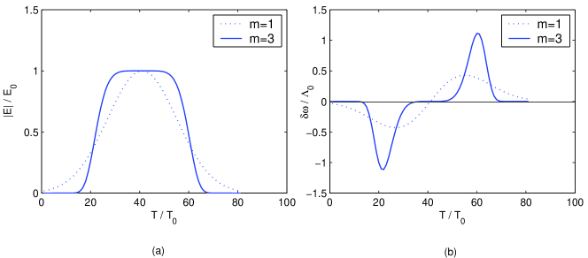
Figure 2: (color online) (a). Envelop of the input probe light, where $E={\cal E}(T)$ and $E_{0}=|{\cal E}(0)|$ is the maximum of the amplitude. The Gaussian probe field ($m=1$, dot-dashed curve), and super Gaussian probe field ($m=3$, solid curve). (b). Frequency chirp of the output atom laser under the case of Gaussian input probe field (for $m=1$) and super Gaussian field (for $m=3$).

Figure 3: (color online) Second-order soliton splits into two solitons under the influence of background amplitude decreasing according to the maximum amplitude of a dispersively spreading Gaussian pulse shown in fig.2(a) (dot-dashed curve). (a) Under a constant parameter $\eta=0.5$; (b) The evolution of soliton phase angle is considered.

References

- [1] M.-O. Mewes et al., Phys.Rev.Lett., 78,582(1997); M. R. Andrews et al., Science 275,637(1997).
- [2] J. Baudon et al., J. Phys. B: At. Mol. Opt. Phys. 32, R173 (1999); A. Peters et al., Metrologia 38, 25 (2001); Y. Shin et al., Phys. Rev. Lett. 92,050405(2004).
- [3] C. Santarelli et al. Phys. Rev. Lett., 82,4619(1999); S. F. Huelga et al., Phys. Rev. Lett., 79,3865(1997); A. Kuzmich et al., Phys. Rev. Lett., 85,1594(2000).
- [4] P. D. Drummond et al., Phys. Rev. A 63,053602(2001).
- [5] W. P. Zhang et al., Phys. Rev. Lett. 72, 60 (1994).
- [6] P. Leboeuf et al, Phys. Rev. A 68, 063608 (2003).
- [7] K. Porsezian et al, Eds. Optical Solitons (Springer-Verlag, Berlin Heidelberg 2003).
- [8] M. J. Werner, Phys. Rev. Lett. 81, 4132(1998); M. Fiorentino et al., Phys. Rev. A 64, R031801 (2001).
- [9] M. W. Zwierlein, et al., Phys. Rev. Lett. 92, 120403 (2004); and references therein. Note that the Feshbach resonance point was remarkably proved to be most stable in this new experimental work. For previous different works, see e.g., E. A. Donley et al., Nature 412, 295 (2001).
- [10] L.V.Hau et al., Nature (London) 397,594(1999); C. Liu et al., Nature (London) 409,490(2001); D. F. Phillips et al., Phys. Rev. Lett. 86,783(2001); M. Bajcsy et al., Nature (London) 426,6967(2003).
- [11] M. D. Lukin et al., Phys. Rev. Lett. 84, 1419(2000); M. D. Lukin et al., Phys. Rev. Lett. 84, 4232(2000).
- [12] Y. Wu et al., Phys. Rev. A 67, 013811 (2003); Y. Wu et al. Deng, Opt. Lett. 29, 2064 (2004); X. J. Liu et al, Phys. Rev. A, 70, 055802 (2004).
- [13] M. Fleischhauer and M.D.Lukin, Phys. Rev. Lett. 84, 5094 (2000); M.Fleischhauer and M.D.Lukin, Phys. Rev. A 65,022314 (2002); C. P. Sun et al, Phys. Rev. Lett. 91,147903 (2003).
- [14] S. E. Harris et al., Phys. Rev. A 46, R29 (1992); M. O. Scully et al, Quantum Optics (Cambridge University Press, Cambridge 1999).
- [15] M. Fleischhauer and S. Q. Gong, Phys. Rev. Lett. 88, 070404 (2002)
- [16] X. J. Liu et al, Phys. Rev. A, 70,015603(2004).
- [17] S. A. Morgan et al, Phys. Rev. A 55,4338(1997); W. P. Reinhardt et al, J. Phys. B 30,L785(1997).
- [18] T. Busch et al, Phys. Rev. Lett., 84,2298(2000).
- [19] J. Denschlag et al., Science, 287,97(2000).
- [20] E. N. Tsoy et al., Phys. Rev. E 62,2882(2000); M. Desaix, Phys. Rev. E 65,056602(2002). S. Zamith et al., Phys. Rev. Lett., 87,033001(2001); G. P. Djotyan et al., Phys. Rev. A 68,053409(2003).
- [21] M. Mašalas and M. Fleischhauer, Phys. Rev. A, 69(RP), 061801(2004).
- [22] G. Juzeliūnas and P. Öhberg, cond-mat/0402317(2004).
- [23] F. Dalfovo et al, Rev. Mod. Phys. 71,463(1999).
- [24] Y. S. Kivshar et al., Rev. Mod. Phys., 61,763(1989).
- [25] Y. S. Kivshar et al., Phys. Rev. E, 49,1657(1994).
- [26] S.Burger et al., Phys. Rev. Lett. 83,5198(1999).
- [27] J. Dziarmaga et al., Phys. Rev. A 66,043615(2002); C. K. Law, Phys. Rev. A 68,015602(2003); B. Damski, Phys. Rev. A 69,043610(2004).
- [28] X. J. Liu et al, arXiv:quant-ph/0403171(2004).
- [29] C. Regal et al, Phys. Rev. Lett., 92,040403(2004).