Casimir Effects: An Optical Approach
I. Foundations and Examples

Abstract

We present the foundations of a new approach to the Casimir effect based on classical ray optics. We show that a very useful approximation to the Casimir force between arbitrarily shaped smooth conductors can be obtained from knowledge of the paths of light rays that originate at points between these bodies and close on themselves. Although an approximation, the optical method is exact for flat bodies, and is surprisingly accurate and versatile. In this paper we present a self-contained derivation of our approximation, discuss its range of validity and possible improvements, and work out three examples in detail. The results are in excellent agreement with recent precise numerical analysis for the experimentally interesting configuration of a sphere opposite an infinite plane.

I Introduction

Revolutionary new experimental techniques have made possible precise measurements of Casimir forcesexpt1 . Casimir’s original prediction for the force between grounded conducting plates due to modifications of the zero point energy of the electromagnetic field has already been verified to an accuracy of a few percent. Variations with the conductor geometry and the effects of finite conductivity and finite temperature will soon be measured as well. Progress has been slower on the theoretical side. Despite years of effort, Casimir forces can only be calculated for the simplest geometries. Beyond Casimir’s original study of parallel platesCasimir , we are only aware of useful calculations for a corrugated plateKardar and for a sphere and a plateGies03 . The former was obtained with functional integral techniques quite special to that geometry and the latter was obtained by computationally intensive numerical methods. Simple and experimentally interesting geometries like two spheres, a finite inclined plane opposite an infinite plane, and a pencil point and a plane, remain elusive. The Proximity Force ApproximationDerjagin (PFA), which has been used for half a century to estimate the dependence of Casimir forces on geometry, was shown by Gies et al. Gies03 to deviate significantly from their precise numerical result for the sphere and plane. Thus at present neither exact results nor reliable approximations are available for generic geometries. It was in this context that we recently proposed a new approach to Casimir effects based on classical opticspap1 . The basic idea is extremely simple: first the Casimir energy is recast as a trace of the Green’s function; then the Green’s function is replaced by the sum over contributions from optical paths labelled by the number of (specular) reflections from the conducting surfaces. The integral over the wave numbers of zero point fluctuations can be performed analytically, leaving

$${\cal E}_{\rm opt}=-\frac{\hbar c}{2\pi^{2}}\sum_{r}(-1)^{r}\int_{{\cal D}_{r}}d^{3}x\frac{\Delta_{r}^{1/2}(x)}{\ell_{r}^{3}(x)}.$$ (I.1)

Here $\ell_{r}(x)$ is the length of the closed geometric optics ray beginning and ending at the point $x$ and reflecting $r$ times from the surfaces. $\Delta_{r}(x)$ is the enlargement factor of classical opticsBorn ; Kline , also associated with the $r$-reflection path beginning and ending at $x$. ${\cal D}_{r}$ is the subset of the domain, ${\cal D}$, between the plates in which $r$ reflections can occur. The factor $(-1)^{r}$ implements a Dirichlet boundary condition on the plates; different boundary conditions require different factors. Both $\ell_{r}(x)$ and $\Delta_{r}(x)$ are very easy to compute either analytically in simple cases, or numerically in general. $\Delta_{r}(x)$, although well known in optics, may not be familiar in the context of Casimir effects. We will describe its properties in some detail.

Eq. (I.1) turns out to be a powerful tool to compute Casimir effects for generic geometries, and to identify, interpret and dispose of, divergences. Eq. (I.1) is not exact. Instead it is an approximation which is valid when the natural scales of diffraction are large compared to the scales that measure the strength of the Casimir force. In practice this will typically be measured by the ratio of the separation between the conductors, $a$, to their curvature, $R$. Although approximate, the optical approach is surprisingly accurate, as well as physically transparent and versatile. It generalizes naturally to the study of Casimir thermodynamics, to the study of energy, pressure, and momentum densities, to various boundary conditions, to fermions, and to compact and/or curved manifolds. This is the first in a series of papers intended to provide an introduction to the optical approach to Casimir physics. Here we will focus on fundamentals: how to derive the optical approximation and how to apply it to practical calculations of Casimir forces. In later papers in this series we study Casimir effects at finite temperature, the calculation of local observables like the energy density and pressure, and the generalization to conducting and other boundary conditions. Our first aim is to familiarize the reader with the use of the optical approximation, since this method of calculation is unfamiliar. In Section II we present some examples of the use of the optical approximation. First we review in more detail the treatment of parallel plates already presented in Ref. pap1 . Although it is no great triumph to rederive this classic result, the optical derivation illustrates several characteristic features of the method: rapid convergence, simple disposal of divergences and ease of computation, in particular. Next we present the case of a sphere and a plate. This too was summarized in Ref. pap1 . Here we concentrate especially on the enlargement factor, both its interpretation and how to compute it. Also we illustrate the generic way that divergences can be eliminated. The numerical results we present here are more accurate than those of Ref. pap1 . Finally we apply the optical method to the case of a finite plate suspended above an infinite conducting plane – the “Casimir pendulum”. We show how all reflections can be computed and how the optical result differs from the proximity force approximation. In collaboration with O. Schroeder we are preparing a thorough study of the hyperboloid (“pencil point”) near an infinite planeSSJ . In Section III we discuss the derivation of the optical approximation from exact expressions for the Casimir energy. We show how a uniform approximation to the propagator turns into a uniform approximation for the Casimir energy. The derivation illustrates the nature of the approximation and shows the way toward improvements, which, in essence, amount to including the effects of diffraction. We present results for a massive scalar field in $N$ dimensions in Section III. Higher spin fields will be considered in a later paper of this series. We discuss the general problem of divergences. The Casimir energy is generically divergent — or more properly, it depends in detail on the cutoffs that limit the conductivity of real materials at high frequency. However it is known that the Casimir force between rigid conductors is cutoff independentGraham:2002xq . In the optical approximation the cutoff dependent terms in the Casimir energy can easily be isolated and shown to be independent of the separation between conductors. They therefore do not contribute to forces and can be dropped. Corrections to the optical approximation will bring in new surface divergences. In Section III.3 we discuss the relation of the optical approximation to previous works on “semiclassical” approximations to the Casimir energySandS . In the last section we summarize our results, discuss their implications, and mention extensions to other interesting geometries.

II Three examples

In this section we present three examples of the use of the optical approximation, eq. (I.1). Our aim is expressly pedagogical: we want to demonstrate that this method can yield interesting and accurate results without onerous calculations.

II.1 Parallel plates

Casimir’s original result for parallel plates can be derived in many ways. We present a derivation from the optical approximation in order to illustrate several generic features of the approach in the simplest possible context. The points we wish to stress are: ease of calculation; the rapid convergence in $r$, the number of reflections; and the simple and accurate treatment of divergences. The “semiclassical” methodSandS and the method of imagesBrown69 generate exactly the same calculation as ours for parallel plates. However they do not generalize to less trivial geometries (although one might say that our method is the correct generalization of the method of images). We study a massless scalar field for simplicity, and quote the generalization to a massive scalar in a later section. For a flat surface the enlargement factor reduces to $1/\ell_{r}(x)$, so the contribution of the $r$ reflection path is

$${\cal E}_{r}=-\frac{\hbar c}{2\pi^{2}}(-1)^{r}M_{r}\int_{{\cal D}_{r}}d^{3}x\frac{1}{\ell_{r}(x)^{4}},$$ (II.1)

where $M_{r}$ is the multiplicity of the path. It is convenient to separate the paths into “odd” ($r=2n+1$) and “even” ($r=2n$) according to the number of reflections. Some of these paths are shown in Fig. [1]. Odd and even paths differ dramatically in their contribution to the Casimir effect: they differ in sign and in multiplicity: $M_{r}=1$ for odd paths and $M_{r}=2$ for even paths, as shown in the figure. The length of an even path depends only on $n$, whereas the length of an odd path varies with position. Finally, odd paths contribute a divergence to ${\cal E}$, but do not contribute to the Casimir force. The even paths are finite and give the entire Casimir force.

Figure 1: Optical paths for parallel plates. The initial and final points on the paths, which coincide, have been separated so the paths can be seen. a) Even reflections 2, 4, and 6. Path 2’ is distinct from 2 and illustrates the origin of $M_{2n}=2$. b) Odd reflection paths. The paths shown form a family of continuously increasing length. Another family begins with the first reflection from the top.

First consider the even paths. The length of the $2n$ reflection path is $\ell_{2n}=2na$ independent of $x$, as can easily be seen in Fig [1]. The volume of each domain, ${\cal D}_{2n}$, is the volume between the plates, $Sa$. Hence the contribution from even paths is

$${\cal E}_{{\rm even}}=-\frac{\hbar c}{2\pi^{2}}2Sa\sum_{n=1}^{\infty}\frac{1}{(2na)^{4}}=-\frac{\hbar c\pi^{2}}{1440a^{3}}S.$$ (II.2)

which is the famous result due to Casimir Casimir . Next consider the odd paths. There are two families. One is illustrated in Fig. 1. The other family begins with the first reflection from the top plate. Their contributions are identical, giving an overall factor of two. The $r=2n+1$ reflection paths range in length from $2na$ to $2(n+1)a$ as can be seen from Fig. [1], and contribute

$${\cal E}_{2n+1}=\frac{\hbar c}{2\pi^{2}}2S\int_{na}^{(n+1)a}dz\frac{1}{(2z)^{4}},\ \mbox{for}\ n=0,1,2,\ldots$$ (II.3)

The first reflection contribution diverges at the lower limit. As discussed in the Introduction (and further in Section III) the divergence indicates dependence on the properties of the material composing the plates and is cutoff at a distance scale $\epsilon$ determined by the microphysics. For example we can take $\epsilon$ to be the skin depth or regard $\epsilon$ as $\sim c/\Lambda$, where $\Lambda$ is a frequency cutoff, for example the plasma frequency of the metal. Inserting $\epsilon$ as the lower limit for $n=0$ and summing over $n$, we obtain the contribution of odd paths,

$${\cal E}_{\rm odd}=\frac{\hbar c}{2\pi^{2}}2S\int_{\epsilon}^{\infty}dz\frac{1}{(2z)^{4}}=\frac{\hbar c}{48\pi^{2}\epsilon^{3}}S$$ (II.4)

This contribution displays the cubic surface divergence expected for a scalar field obeying a Dirichlet boundary conditionDeutsch79 . However, the divergent term — and indeed the sum of all odd reflections — is independent of $a$ and therefore does not contribute to the force between the plates. Until now we have not considered the contributions from one-reflection paths that lie below the bottom plate or above of the top plate. It is easy to see that the sum of these contributions is identical to eq. (II.4) and does not contribute to the force. This simple calculation illustrates some general features of the optical approach:

• The even reflections dominate, give rise to attraction, and their sum converges rapidly in $n$. They are also attractive for Neumann boundary conditions, where the factor $(-1)^{r}$ is absent. They would be repulsive if one surface were Neumann and the other Dirichlet. In the case of parallel plates 92% of the Casimir effect comes from the second reflection, 98% from the second and fourth, and 99.3% from the second, fourth and sixth reflections. Similar results will be found to hold in more complicated geometries.

• The only divergent contribution comes from the first reflection. It does not depend on the separation and therefore does not contribute to the Casimir force. This result is quite general. To see the general argument, reconsider the first reflection from the bottom plate, ${{\cal S}_{1}}$

  $${\cal E}_{1,{\cal S}_{1}}=\frac{\hbar c}{2\pi^{2}}S\int_{\epsilon}^{a}dz\frac{1}{(2z)^{4}}=\frac{\hbar c}{2\pi^{2}}S\int_{\epsilon}^{\infty}dz\frac{1}{(2z)^{4}}-\frac{\hbar c}{2\pi^{2}}S\int_{a}^{\infty}dz\frac{1}{(2z)^{4}}.$$ (II.5)

  The first term in eq. (II.5) combined with the contribution of the 1-reflection path outside of the plates (from the lower face of the bottom plate) is the cutoff dependent energy of an isolated plate. It is manifestly independent of the presence of any other conductor, and gives no contribution to Casimir forces. The second term is a finite effect of the first reflection. For parallel plates the finite contribution of the first reflection is cancelled by higher odd reflections. This occurs whenever the enlargement factor is $1/\ell_{n}^{2}$, that is, when all the conductors are planar. For non-planar surfaces the first reflection gives a (relatively small) cutoff independent contribution to the force.

• The optical approach gives the exact answer for infinite plates. However it will fail when $S^{1/2}\approx a$ for the same reason that the capacitance of two finite, parallel metallic plates contains corrections of order $a^{2}/S$Feynmanlect : It is a poor approximation to consider the electric field inside two far separated plates ($a\gtrsim S^{1/2}$) as constant inside and zero outside. Likewise, in the same limit it is a poor approximation to expect the Green’s function for the field $\phi$ to have contributions only from optical paths. The corrections, or edge effects, can be regarded as due to diffractive rays coming from the edges of the plates Keller . We discuss corrections to the optical approximation in further detail in Section III.

• The difference between even and odd paths has a fundamental origin, as already noticed in work on the “semiclassical” approximation to the Casimir energy SandS . The even paths are truly periodic, in the sense that the momentum of the particle, after going around the path, returns to its initial value. These are therefore the paths that according to Gutzwiller Gutz contribute most to the oscillations of the density of states. The connection between these paths, the oscillation of the density of states, and the finite part of the Casimir energy has been noted many timesFulling and is exact for parallel plates and related geometries (eg. flat manifolds with various topologies). However, the exactness of this result is an accident due to the particularly simple geometry. For example, there are very simple geometries in which periodic paths do not exist at all (eg. the Casimir pendulum: a finite plane inclined at an angle above an infinite surface). The relation between the optical approach and the “semiclassical” approach is discussed further in Section III.

II.2 The sphere and the plane

Next we analyze a problem with non-planar conductors — typical of real experimental configurationsexpt1 — a sphere of radius $R$ separated by a distance $a$ from an infinite plane. In Ref. pap1 we tested the optical approximation by computing the Casimir force between a sphere and a plane up through the fourth reflection. We showed that the optical approximation is in very good agreement with the numerical results of Ref. Gies03 for $a/R\lesssim 1$. In fact the numerical results presented in Ref. pap1 suffered from an insufficiently accurate numerical integration algorithm. The results presented here supercede Ref. pap1 and show that the optical approximation is even more accurate than we originally claimed. For example, the optical approximation and the numerical data differ by only 30% at $a/R\approx 5$. Here we explain in detail how to compute the first and second reflection contributions. The relevant paths are shown along with some other aspects of the geometry in Fig. 2.

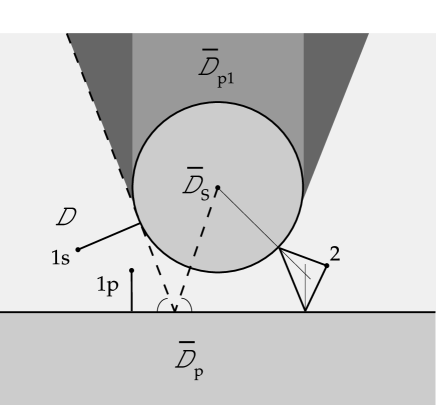
Figure 2: Geometry and reflections for a sphere and a plane. The regions and geometrical constructions are defined in the text.

For each reflection we must compute a) the optical path length, $\ell_{r}(x)$, b) the enlargement factor, $\Delta_{r}(x)$, and c) the domain of integration ${\cal D}_{r}$ for which $r$-reflections are possible. The ${\cal D}_{r}$ are subsets of the domain ${\cal D}$ above the plane and outside the sphere.

II.2.1 Optical path lengths, $\ell_{r}(x)$

Finding the $r$-reflection optical path from $x$ back to $x$, $\ell_{r}(x)$, is elementary in principle. One just draws straight lines from $x$ to a given surface, from the arrival point on this surface to another surface, and so on, returning after $r$ reflections to the original point $x$. One then moves the points of reflection on the surfaces until one reaches the minimum total length (an elastic string would do the job). The minimum length path suffers specular reflection upon each encounter with a surface. In all but the simplest geometries this problem must be solved numerically. However it is a problem amenable to extremely quick numerical solution: it is easily defined and the minimum is unique (at least for convex surfaces). This procedure also defines the points of reflection, $x_{r,1}(x)$, $x_{r,2}(x)$, etc. The first reflection paths from the sphere ($1s$) and the plane ($1p$) and the two reflection path are shown in Fig. (2).

II.2.2 Enlargement factor, $\Delta_{r}(x)$

The enlargement factor for the closed path beginning and ending at $x$ is a special case of the general enlargement factor, $\Delta_{r}(x,x^{\prime})$ for propagation from $x$ to $x^{\prime}$, well known in opticsBorn ; Kline . In another guise, it is also well known to field theorists: $\Delta_{r}(x,x^{\prime})$ is just the van Vleck determinant arising from the Gaussian fluctuations of the action about the classical $r$-reflection path from $x$ to $x^{\prime}$. In Section III, where we discuss the origins of the optical approximation, we show that the evaluation of the determinant gives the standard optics definition,

$$\Delta_{r}(x,x^{\prime})=\frac{d\Omega_{x}}{dA_{x^{\prime}}}$$ (II.6)

From this definition it is clear that in order to obtain $\Delta_{r}(x,x^{\prime})$ one must follow the spread of an infinitesmal pencil of rays of opening $d\Omega_{x}$ from their origin at $x$, along this path, and measure the spread in area $dA_{x^{\prime}}$ when they arrive at $x^{\prime}$. Having already identified the points of reflection in II.2.1 it is relatively easy to compute $\Delta(x,x^{\prime})|_{x^{\prime}=x}$ numerically by tracing the paths of a few nearby raysSSJ . It is also possible to solve this problem analytically. Here we present the analytic solution for the first and second reflections from a sphere and plane. Beyond this level, it is probably more efficient to proceed numerically. One reflection from the plane is trivial: $\Delta(x,x)=1/\ell^{2}_{1}(x)$ One reflection from the sphere is simplified by a) normal incidence, and b) $x=x^{\prime}$. The second reflection can be simplified by regarding it as a single reflection from the sphere starting from $x$ and ending at the image $\tilde{x}$ of the original point $x$ in the plane. In that case we need $\Delta_{1}(x,\tilde{x})$. Consider the path from $x$ to the sphere at the point $Q$, and then to $x^{\prime}$. To obtain $\Delta$ one must follow the wavefront radii of curvature along the ray. We consider a ray that impacts the sphere at an angle $\theta$ to the normal. It travels a distance $\sigma_{1}$ before and $\sigma_{2}$ after, with $\ell=\sigma_{1}+\sigma_{2}$. These variables are defined in Fig. 3(a). Consider a pencil of rays originating at $x$, spanning two infinitesmal arcs of angular widths $d\phi_{1,2}$ along perpendicular directions. Let $dx_{1}^{\prime}$ and $dx_{2}^{\prime}$ be the associated arc lengths observed at $x^{\prime}$. Then

$$\Delta_{r}(x)=\left.\frac{d\Omega_{x}}{dA_{x^{\prime}}}\right|_{x^{\prime}=x}=\left.\frac{d\phi_{1}}{dx_{1}^{\prime}}\frac{d\phi_{2}}{dx_{2}^{\prime}}\right|_{x^{\prime}=x}.$$ (II.7)

Since both the initial ray and the sphere have equal radii of curvature we have the freedom to choose the directions defining $d\phi_{1}$ and $d\phi_{2}$. We choose “latitude” and “longitude” as follows: Latitude is the direction perpendicular to the plane formed by $x$, $x^{\prime}$ and the center of the sphere (see Fig. 3(a)). Longitude is the direction in the plane.

  

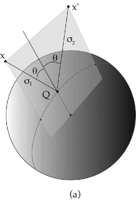
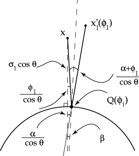
Figure 3: Geometry for reflection in a sphere. (a) The ray from $x$ to $x^{\prime}$ reflecting at $Q$. Nearby rays originating at $x$ and lying in the plane vary in longitude. Nearby rays out of the plane vary in latitude. (b) Variables for the calculations of the enlargment factor associated with latitude. The $xx^{\prime}$ plane has been projected along the vertical. A nearby ray originating at $x$ heading out of the $xx^{\prime}Q$ plane by an angle $\phi_{1}$ is shown. This ray reflects from the sphere at $Q(\phi_{1})$. The angle subtended by $x$ and $Q(\phi_{1})$ from the center of the sphere is $\beta$. The angle formed by the vector from the center of the sphere to $x$ and the ray from $Q(\phi)$ to $x^{\prime}_{1}(\phi_{1})$ is $\alpha$. In the diagram the distance $\sigma_{1}$ and the angles $\alpha$ and $\phi_{1}$ are modified by factors of $\cos\theta$ due to the projection.

Consider the pencil of rays of varying latitude as shown in Fig. 3(b). The variables are defined in the figure. It is easy to see that

$${dx_{1}^{\prime}}={\sigma_{1}d\phi_{1}+\sigma_{2}d\alpha},$$ (II.8)

and considering that $d\alpha=2d\beta\cos\theta+d\phi_{1}$ and $Rd\beta=\sigma_{1}d\phi_{1}$, we find

$$\frac{d\alpha}{d\phi_{1}}=1+\frac{2\sigma_{1}\cos\theta}{R},$$ (II.9)

and hence

$$\frac{d\phi_{1}}{dx_{1}^{\prime}}=\frac{1}{\ell+\frac{2\sigma_{1}\sigma_{2}\cos\theta}{R}}$$ (II.10)

The same calculation applies for the longitudinal displacement except that the relation between $d\phi_{1}$ and $d\beta$ is replaced by $Rd\beta=\ \sigma_{1}d\phi_{2}/\cos\theta$ and $d\alpha=2d\beta+d\phi_{1}$, with the result

$$\frac{d\phi_{2}}{dx_{2}^{\prime}}=\frac{1}{\ell+\frac{2\sigma_{1}\sigma_{2}}{R\cos\theta}}$$ (II.11)

Putting these formulas together we find for a single reflection on the sphere (the subscript $s$ indicates reflection from the sphere) with angle of reflection $\theta$

$$\Delta_{1s}(x,x^{\prime})=\frac{1}{(\ell+\frac{2\sigma_{1}\sigma_{2}}{R\cos\theta})(\ell+\frac{2\sigma_{1}\sigma_{2}\cos\theta}{R})}.$$ (II.12)

Note that $\Delta(x,x^{\prime})$ is symmetric with respect to the interchange of $x$ and $x^{\prime}$ as it must, because the propagator possesses this symmetry. For the first reflection from the sphere we have $\cos\theta=1$ and $\sigma_{1}=\sigma_{2}=\ell/2$, so

$$\Delta_{1s}(x)=\frac{1}{(\ell+\ell^{2}/2R)^{2}}$$ (II.13)

and, as mentioned above, the enlargement factor for the second reflection (on the sphere and then on the plane or vice versa), is given by the first reflection from $x$ to its image $\tilde{x}$ in the plane, $\Delta_{2}(x)=\Delta_{1s}(x,\tilde{x})$. A similar approach to higher reflections would require further analysis. The original wavefront leaving $x$ is spherical. The first reflection from the sphere produces a new wavefront with, in general, two unequal radii of curvature. When next incident upon the sphere, the asymmetric wavefront will be transformed in a manner yet to be described. The ease with which $\Delta_{r}(x)$ can be computed numerically makes this unnecessary.

II.2.3 Domain of the $r^{\rm th}$ reflection, ${\cal D}_{r}$

The next step is the integration over the domains appropriate to each reflection. The first reflections give rise to cutoff dependent but $a$-independent contributions which must be analyzed at this point. Consider the first reflection from the plane. The appropriate domain is all of space except the interior of the sphere $\overline{{\cal D}}_{s}$ and the region shadowed by the sphere $\overline{{\cal D}}_{p1}$ (see Fig. 2). The integral can then be written as the difference between the integral over all space and the integral over $\overline{{\cal D}}_{s}\bigcup\overline{{\cal D}}_{p1}$. The integral over the whole space is the divergent constant discussed in II.1 which does not contribute to the force. It is to be ignored in the following. So the correct domain for the first reflection from the plane is the region, $\overline{{\cal D}}_{s}\bigcup\overline{{\cal D}}_{p1}$, in the shadow of the sphere, and the sign is to be reversed. Similarly, the integral of the first reflection on the sphere must be performed on the domain consisting of the whole space minus the interior of the sphere ($\overline{{\cal D}}_{s}$) and the region below the plate ($\overline{{\cal D}}_{p}$). The irrelevant divergence is given by the integral over all the space minus the interior of the sphere and the finite, $a$-dependent part, which contributes to the Casimir force, is given by the negative of the integral over the region, $\overline{{\cal D}}_{p}$, below the plane. So the correct domain for the first reflection from the sphere is $\overline{{\cal D}}_{p}$ and the sign of the contribution is reversed. Hence we can write

$${\cal E}_{1s}+{\cal E}_{1p}=-\frac{\hbar c}{2\pi^{2}}\int_{\overline{{\cal D}}_{s}\bigcup\overline{{\cal D}}_{p1}}d^{3}x\frac{1}{(2z)^{4}}-\frac{\hbar c}{2\pi^{2}}\int_{\overline{\cal D}_{p}}d^{3}x\frac{\Delta_{1s}^{1/2}(x)}{\ell_{1s}^{3}(x)}.$$ (II.14)

The second reflection gives a finite contribution to ${\cal E}$. The path length, $\ell_{2}(x)$, never vanishes so there are no divergences at short distances, and the integrand, $\Delta_{2}^{1/2}(x)/\ell^{3}(x)$, falls rapidly at large distances. The result is typically approximately $90\%$ of the total result. Higher reflections can be analyzed in a similar fashion. The integration domains become progressively more restricted. For example, three reflection paths that reflect twice from the plane and once from the sphere do not exist in the shadow of the sphere ($\overline{{\cal D}}_{p1}$) nor in the darkly shaded regions in Fig. 2 determined by the geometrical construction indicated by the dashed lines. It is not hard to carry out the constructions and calculations necessary to construct the optical approximation for the sphere and plane to any required order.

II.2.4 Discussion of numerical results

In Ref. pap1 we presented initial results on the optical approximation for the sphere and plane. Here we present final results (see Fig. 4), discuss them in more detail, and compare them with the results of Ref. Gies03 and with the proximity force approximation (PFA). In presenting our results we display the sum of all the reflections (even and odd) up to (and including) the fourth. Since the energy must approach the parallel plate limit as $a\to 0$ we can estimate the error in neglecting higher reflections in this limit. The error in neglecting the fifth and higher odd reflections is a $+3.8\%$ excess (because the sign of the odd reflections contribution is opposite to that of the total energy) as $a\to 0$. Neglecting the even reflections (6th, 8th, etc.) as $a\to 0$ gives an error of $-1.8\%$, negative because these contributions have the same sign of the total energy. Altogether the sum of the first four reflections overestimates the energy by $3.8\%-1.8\%=2\%$ as $a\to 0$. To illustrate this estimate of accuracy we have plotted our results as a band $2\%$ in width in Fig. 4. Since the fractional contribution of higher reflections decreases with $a$, we believe this is a conservative estimate for larger $a$. Obviously, calculating the higher reflections will reduce this uncertainty interval, leaving eventually only the error due to diffraction which we are not able to estimate. The proximity force approximation has been the standard tool for estimating the effects of departure from planar geometry for Casimir effects for many yearsMT . In this approach one views the sphere and plate as a superposition of infinitesimal parallel plates:

$${\cal E}_{\rm PFA}=-\frac{\pi^{2}\hbar c}{1440}\int_{{\cal S}}d^{2}S\frac{1}{d(x)^{3}}.$$ (II.15)

where $d(x)$ is the distance from the plate to the sphere at a point $x$ on the surface ${\cal S}$. This formulation is ambiguous since the surface ${\cal S}$ could be taken to be either the sphere or the plate. Whichever surface is chosen, the distance is measured normal to that surface. The ambiguity is useful since it gives a measure of the uncertainty in the PFA. In either case the relevant integrals are easily performed. For the plate we obtain,

$${\cal E}_{\rm PFA}^{\rm plate}=-\frac{\pi^{3}\hbar cR}{1440a^{2}}\frac{1}{1+a/R}$$ (II.16)

while for the sphere we obtain

$${\cal E}_{\rm PFA}^{\rm sphere}=-\frac{\pi^{3}\hbar cR}{1440a^{2}}\left(1-3\frac{a}{R}-6\frac{a^{2}}{R^{2}}\left(1+(1+\frac{a}{R})\ln\frac{a}{R+a}\right)\right)$$ (II.17)

In the limit $a/R\to 0$ both estimates agree to lowest order. The $a\to 0$ limit is usually called the proximity force theorem and has been much discussed over the years. It is usually stated as a result for the Casimir force in the limit $a/R\to 0$: ${\cal F}_{\rm PFA}\sim 2\pi R{\cal E}/A=-\pi^{3}\hbar cR/720a^{3}$ (where ${\cal E}/A$ is the Casimir energy per unit area for parallel plates). This limit provides a convenient parametrization of the Casimir force when $a$ is not so small,

$${\cal F}=-f(\frac{a}{R})\frac{\pi^{3}\hbar cR}{720a^{3}}$$ (II.18)

Modern experiments are approaching accuracies where the deviations of $f(a/R)$ from unity may be important. The accuracy of the PFA beyond the $a/R\to 0$ limit is unknown, and the two different versions give different ${\cal O}(a/R)$ corrections:

$$f_{\rm PFA}^{\rm plate}(a/R) = 1-\frac{1}{2}\frac{a}{R}+{\cal O}(\frac{a^{2}}{R^{2}})$$ (II.19)

$$f_{\rm PFA}^{\rm sphere}(a/R) = 1-\frac{3}{2}\frac{a}{R}+{\cal O}(\frac{a^{2}}{R^{2}})$$ (II.20)

An important application of the optical approximation is to obtain a more accurate estimate of $f(a/R)$. The optical approximation to the Casimir energy and the data of Ref. Gies03 both fall like $1/a^{2}$ at large $a$. In fact both are roughly proportional to $1/a^{2}$ for all $a$. In contrast the PFA estimates of the energy falls like $1/a^{3}$ at large $a$ and depart from the Gies et al data at relatively small $a/R$. For purposes of display we therefore scale the estimates of the energy by the factor $-1440a^{2}/\pi^{3}R\hbar c$. The results are shown in Fig. 4.

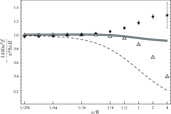
Figure 4: Casimir energy for a sphere of radius $R$ a distance $a$ above an infinite plane. $1440a^{2}{\cal E}/\pi^{3}R\hbar c$ is plotted versus $a/R$. The stars with error bars are the data of Ref. Gies03 . The thick solid curve is the optical approximation through the fourth reflection. The width of the curve indicates our estimate of the error in the optical approximation from neglect of the odd and even reflections with $n\geq 5$. The dashed curve is the plate-based proximity force approximation. The triangles are the results we published in Ref. pap1 , which are superceded by this work.

At large $a/R$ the optical approximation has the same scaling behavior as the data and differs from Ref. Gies03 by no more than 30% at the largest $a/R$. At small $a/R$, given our estimate of the accuracy of the optical approximation, we find that

$$f^{\rm optical}(a/R)=1+0.05a/R+{\cal O}\left((a/R)^{2}\right),$$ (II.21)

which must be compared with the predictions of PFA eqns.(II.19) and (II.20). In Fig. 5 we show the contributions to the optical approximation of the different reflections we have computed. As expected the dominant contribution, always greater than 90%, comes from the second reflection. The fourth reflection contributes about 6% for $a/R\ll 1$ and less as $a/R$ increases. The contributions of the first and third reflections are very small for all $a/R$. A relevant result, confirmed by the analytical analysis on the energy momentum tensor (within the optical approximation), the subject of the second paper of this series, is that the asymptotic behavior of ${\cal E}$ as $a/R\gg 1$ predicted by the optical approximation is $\propto 1/a^{2}$. This is in contrast with the Casimir-Polder law which predicts $1/a^{4}$ at large $a$ the discrepancy is to be attributed to diffraction effects.

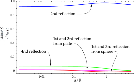
Figure 5: Contributions of specific reflections to the optical approximation.

II.3 Casimir Pendulum

In this section we treat a problem for which the exact answer is unknown. The configuration is shown in Fig. 6. The base plate is taken to be infinite. The upper plate is held at its midpoint a distance $a$ above the base plate. The width of the upper plate is $w$ and its depth, $d$ (out of the page), is assumed to be infinite. We define the Casimir energy per unit depth, $\varepsilon={\cal E}/d$. $\theta$ is the angle of inclination of the upper plate. It will be convenient to use $z=\tiny{\frac{1}{2}}w\sin\theta$ as a variable as well. It is also possible to view this configuration as a finite slice between $\ell_{1}=a/\sin\theta-w/2$ and $\ell_{2}=a/\sin\theta+w/2$ of a wedge of opening angle $\theta$. In this section we will discuss both the Casimir energy and the “Casimir torque”, $\nu=\frac{1}{d}\frac{d{\cal E}}{d\theta}$, per unit depth.

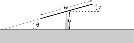
Figure 6: Geometry for the Casimir Pendulum.

We are aware of two ad hoc approximate approaches to this problem. The first is the PFA which treats each element of the system perpendicular to the lower plate as an infinitesmal parallel plate Casimir system. It is easy to show that

$$\varepsilon_{\rm PFA} = -\frac{\pi^{2}\hbar c}{1440}\frac{w\cos\theta}{a^{3}}\left(1-\frac{w^{2}\sin^{2}\theta}{4a^{2}}\right)^{-2}$$ (II.22)

$$= -\frac{\pi^{2}\hbar ca}{1440}\frac{\sqrt{w^{2}-4z^{2}}}{(a^{2}-z^{2})^{2}}$$

which gives a torque,

$$\nu_{\rm PFA}(a,w,z)=-\frac{\pi^{2}\hbar c}{720}\ \frac{az(w^{2}-a^{2}-3z^{2})}{(a^{2}-z^{2})^{3}}$$ (II.23)

where the minus sign denotes that the torque is destabilizing: $z=0$ is a point of unstable equilibrium. As in the case of the sphere and the plane, the PFA is ambiguous. A more symmetric treatment of the two planes in the present geometry would integrate over the surface that bisects the wedge and take the distance normal to that surface. The result is the replacement of $\cos\theta$ by $\cos^{4}(\theta/2)$ in eq. (II.22) and a similar modification of the torque. A second “approximate” treatment of the Casimir Pendulum can be extracted from the known exact solution for the Casimir energy density for the “Dirichlet wedge”dirichletwedge , which consists of two semi-infinite plates with opening angle $\theta$ meeting at the origin. One can obtain an estimate of the energy for the pendulum by integrating the energy density over the two dimensional domain bounded (in polar coordinates, $(\rho,\phi)$) by $0<\phi<\theta$ and $\ell_{1}<\rho<\ell_{2}$. This approach takes no account of the modification of the energy density due to the finitenss of the upper plate. Furthermore it is inherently ambiguous because the energy density for a scalar field is only defined up to a total derivative. The calculation in Ref. dirichletwedge used the conformally invariant stress tensor. One would obtain a different answer if one used, for example, the Noether stress tensor. In light of these difficulties, we do not pursue this approach further. To compute the optical approximation we need the enlargement factor, the lengths of optical paths, and the integration domain, ${\cal D}_{r}$. Since all the conducting surfaces are planar, the enlargement factor is trivial in this case, $\Delta_{r}(x)\to 1/\ell_{r}^{2}(x)$. The path lengths are also easy to compute. The only non-trivial step is the determination of the integration domains. As in the case of parallel plates, the odd reflections do not contribute to forces or torques for the Casimir pendulum. Instead they sum to a cutoff dependent constant associated with each plate. Any odd reflection path “turns around” with a reflection at normal incidence from one plate or the other. Consider all the points, $x$, which are the origins of paths that turn around at a given point $P$ on either surface. These paths are shown, for the case where $P$ is on the lower, infinite plane, in Fig. 7. They comprise one reflection paths lying on the interval $\overline{PQ_{1}}$, three reflection paths lying on the interval $\overline{Q_{1}Q_{2}}$, etc. The contributions to $\varepsilon$ from these intervals integrates to the same result as the integral over $z$ for odd paths in the case of parallel plates. It is independent of $a$, $w$, and $\theta$ and can be set aside. The fact that the enlargement factor is trivial is crucial for this argument.

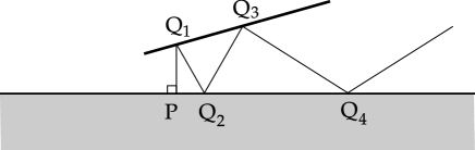
Figure 7: Odd reflection paths for the Casimir Pendulum.

II.3.1 Even optical path lengths, $\ell_{r}(x)$

The analysis of paths that reflect an even number of times makes use of simple geometrical concepts. For any point $x\equiv(\rho,\phi)$, we define an infinite sequence of images in the upper and lower planes as shown in Fig. 8, ignoring for the moment that the upper plane is finite. The images below the lower plane are denoted $\bar{x}_{1},\bar{x}_{2},\ldots$ and those above the upper plane are denoted $x_{1},x_{2},\ldots$. In sequence, $\bar{x}_{1}={\mathbf{\overline{R}}}x$, $x_{1}=\mathbf{R}x$, $x_{2}=\mathbf{R}\bar{x}_{1}$, $\bar{x}_{2}=\mathbf{\overline{R}}x_{1}$, etc. with $\mathbf{\overline{R}}$ denoting reflection in the lower plane and $\mathbf{R}$ denoting reflection in the upper plane. All of the images lie on the circle of radius $\rho$ about the origin. The length of the $2n$ reflection path can easily be seen to be given by

$$\ell_{2n}(x)=||x_{n}-\bar{x}_{n}||=4\rho^{2}\sin^{2}n\theta$$ (II.24)

independent of $\phi$.

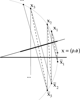
Figure 8: Images of the point $x$ in the Casimir Pendulum configuration. The dashed lines have the same length as the $r=2,4,6,\ldots$ reflection paths.

Substituting into eq. (I.1) we obtain the expression for the Casimir energy per unit depth,

$$\varepsilon_{\rm opt}=-\frac{\hbar c}{16\pi^{2}}\sum_{n=1}^{N_{\rm max}}\frac{1}{\sin^{4}n\theta}\int_{0}^{\theta}d\phi\int_{0}^{\infty}d\rho\frac{1}{\rho^{3}}\ \Theta({\cal D}_{2n})$$ (II.25)

The step function $\Theta({\cal D}_{2n})$ vanishes when the point $x$ is not in the domain where $2n$-reflection paths are possible. As we show in the following section, for $n$ large enough, ${\cal D}_{2n}\to\emptyset$. $N_{\rm max}$, the upper limit on the $n$-sum, is the largest value of $n$ for which any $2n$-reflection paths exist.

II.3.2 Domain of the $2n^{\rm th}$ reflection, ${\cal D}_{2n}$

The domain in which the $2n$-reflection path exists is determined by the constraint that the points of reflection at the upper plate must lie between $\ell_{1}$ and $\ell_{2}$, the inner and outer radii that define its boundaries. Note, of course, that $\ell_{2}>\ell_{1}$. Although the calculation is elementary, it is tricky, so we only quote the results. The constraints depend on whether $n$ is even or odd, so we summarize them independently.

• $n$-odd When $n$ is odd, the integration domain ${\cal D}_{2n}$ is defined by the inequalities:

  $$\ell_{1}\cos\phi\leq\rho\cos n\theta\leq\ell_{2}\cos((n-1)\theta+\phi)$$ (II.26)

  where the lower limit ensures that the innermost reflection occurs at $\rho\geq\ell_{1}$ and the upper limit ensures that the outermost reflection occurs at $\rho\leq\ell_{2}$. The inequality cannot be satisifed for any $\rho$ or $\phi$($\leq\theta$) unless

  $$\ell_{2}\cos(n-1)\theta>\ell_{1}$$ (II.27)

  When eq. (II.27) is satisfied the contribution of the $2n^{\rm th}$ reflection ($n$-odd) is

  $$\varepsilon^{\rm odd}_{{\rm opt}\ n} = -\frac{\hbar c}{32\pi^{2}}\frac{\cos^{2}n\theta}{\sin^{4}n\theta}\left\{\matrix{\frac{1}{\ell_{1}^{2}}\tan\theta-\frac{1}{\ell_{2}^{2}}\left(\tan n\theta-\tan(n-1)\theta\right)&\mbox{for}\ \ \ell_{2}\cos n\theta\geq\ell_{1}\cos\theta\cr\frac{(\ell_{2}\cos(n-1)\theta-\ell_{1})^{2}}{\ell_{1}^{2}\ell_{2}^{2}\ \cos(n-1)\theta\ \sin(n-1)\theta}\qquad\ \ \qquad&\mbox{for}\ \ \ \ell_{2}\cos n\theta\leq\ell_{1}\cos\theta}\right.$$ (II.28)

• $n$-even When $n$ is even, the integration domain ${\cal D}_{2n}$ is defined by the inequalities:

  $$\ell_{1}\cos(\theta-\phi)\leq\rho\cos n\theta\leq\ell_{2}\cos((n-1)\theta+\phi)$$ (II.29)

  where, as before, the lower limit ensures that the innermost reflection occurs at $\rho\geq\ell_{1}$ and the upper limit ensures that the outermost reflection occurs at $\rho\leq\ell_{2}$. The inequality cannot be satisifed at all unless

  $$\ell_{2}\cos(n-1)\theta>\ell_{1}\cos\theta$$ (II.30)

  When eq. (II.30) is satisfied the contribution of the $2n^{\rm th}$ reflection ($n$-even) is

  $$\varepsilon^{\rm even}_{{\rm opt}\ n} = -\frac{\hbar c}{32\pi^{2}}\frac{\cos^{2}n\theta}{\sin^{4}n\theta}\left\{\matrix{\frac{1}{\ell_{1}^{2}}\tan\theta-\frac{1}{\ell_{2}^{2}}\left(\tan n\theta-\tan(n-1)\theta\right)&\mbox{for}\ \ \ell_{2}\cos n\theta\geq\ell_{1}\cr\frac{(\ell_{2}\cos(n-1)\theta-\ell_{1}\cos\theta)^{2}}{\ell_{1}^{2}\ell_{2}^{2}\ \cos(n-1)\theta\ \sin n\theta\ \cos\theta}\qquad\ \ \qquad&\mbox{for}\ \ \ell_{2}\cos n\theta\leq\ell_{1}}\right.$$ (II.31)

The torque is obtained by differentiating with respect to $\theta$ at fixed $a$ and $w$, remembering that $\ell_{1}$ and $\ell_{2}$ depend on $\theta$. Of course the $\theta$-derivative of eqs. (II.31) and (II.28) are complicated and need not be written down explicitly. The resulting expressions for $\nu^{\rm odd}_{{\rm opt}\ n}$ and $\nu^{\rm even}_{{\rm opt}\ n}$ must be summed over $n$ subject to the constraints in eqs. (II.28) and (II.31). This sum must be performed numerically. The results are discussed in the following subsection.

II.3.3 Discussion

Fig. 9 shows the pendulum Casimir energy as a function of $z$ for $a=1$ and several values of $w$. The weak dependence on $z$ at small $z$ is to be expected. So is the divergence as $z\to 1$ which we do not show in the figure. When the plates touch at $z=1$, the Casimir energy of perfectly sharp, perfectly conducting plates would in fact diverge, as would the Casimir torque. The optical approximation for the pendulum turns out to be very close to the plate based PFA. It is convenient therefore to scale out a factor of $-1440a^{3}/\hbar c\pi^{2}w$ (see eq. (II.22)) when displaying or results for the energy per unit depth, $\varepsilon_{\rm opt}$, and a factor $-720a^{5}/\hbar c\pi^{2}w^{2}$ when displaying results for the torque per unit depth.

  

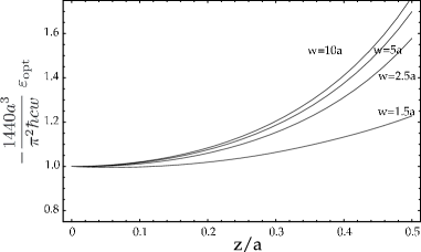
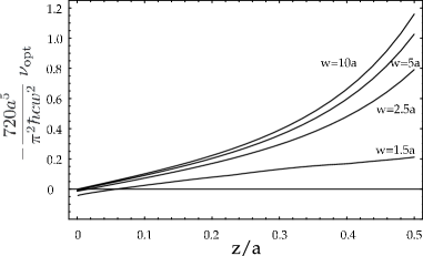
Figure 9: Casimir energy and torque in scaled units for a Casimir pendulum of width $w=1.5a,2.5a,5a$ and $10a$. Positive values of the scaled torque are destabilizing.

The energy and torque are plotted for representative values of $w$ ($w=1.5a,2.5a,5a,$ and $10a$) as a function of $z/a$ in Fig. 9. The plots are shown only up to $z/a=0.5$. Above $z/a\sim 0.5$ both grow rapidly and diverge at $z=a$. The PFA gives an excellent approximation for the pendulum over a wide range of the parameter space. This can be seen by examining the ratio of $\varepsilon_{\rm opt}/\varepsilon_{\rm PFA}$ as shown in Fig. 10. The reason behind this success is that the second (optical) reflection is proportional to the PFA result (eq. (II.22)) for all $z$. The constant of proportionality is the familiar $90/\pi^{4}=0.924$.

  

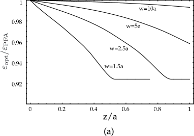
Figure 10: The ratio of the optical approximation to the PFA. (a) for a pendulum of different widths as a function of $z/a$. The breaks in the curves for $w=1.5a$ and $2.5a$ occur when only the second reflection can contribute. The $w=1.5a$ curve ends at the $z=0.75a$ when $z=w/2$. (b) The contributions of the 4th and 6th reflections for $w=2.5a$. The 2nd reflection contributes 0.924…independent of $z$. This is the only case we found in which the optical approximation gives an energy smaller than the PFA.

The sum of the higher even reflections combines with the second to equal the PFA at $z=0$ and drops away slowly with increasing $z/a$. So the optical estimate coincides with the PFA at $z=0$ and drops slowly with $z$. The contributions of the first few reflections are shown for $w=2.5a$ in Fig. 10. A careful study of Fig. 9 reveals one peculiar feature of the optical approximation which is interesting in principle, if not in practice. The torque does not vanish at $z=0$, and therefore the Casimir energy has a cusp at $z=0$. The section of the graph near $z=0$ is enlarged in Fig. 11 to make the effect clearer. The torque starts negative (stabilizing) at very small $z$ before it changes sign and becomes destabilizing as $z$ increases. This is an effect of the finite extent of the upper plate. It vanishes like $a/w$ at large $w$. We are not able to determine whether this is an artifact of the optical approximation’s neglect of diffraction, or whether it is a real effect at small $z$. We know of no theorem that precludes a cusp in the energy at $z=0$. We will have to wait until the effects of diffraction can be included before analyzing this further.

Figure 11: Torque in scaled units for a Casimir pendulum of width $w=1.5a,2.5a,5a$ and $10a$, for $z\approx 0$. Positive values of the scaled torque are destabilizing.

III Origins of the optical approximation

Most studies of Casimir energies do not consider approximations. Instead they focus on ways to regulate and compute the sum over modes, $\sum\frac{1}{2}\hbar\omega$MT . These methods have proved very difficult to apply to geometries other than parallel plates. The main reason for this impasse lies in the requirement of an analytic knowledge of the spectrum. Finding the spectrum of the Laplace operator for non-separable problems is not merely a technical difficulty, it is more one of principle. In fact there are strict relations between this problem and those of chaotic billiards theory. The existence of an exact solution for the Casimir problem with a non-trivial geometry would imply the existence of an exact solution for the same family of quantum billiards and hence of classical billiards. 30 years of work on the ergodicity of classical billiards and the implications for the density of states in the corresponding quantum billiards suggest this task is hopeless (see Gutz ). On the other hand, one could argue that a numerical solution of the Dirichlet problem could easily give the spectrum to some high, but finite, accuracy, and this could be used to compute the Casimir energy. However the Casimir energy diverges – the leading non-trivial divergence in $N$ dimensions is of order $\Lambda^{N}$. The Casimir force between rigid bodies is known to be finite, and one could hope to compute it by introducing a cutoff, computing the energy at nearby separations, $a$ and $a+da$, taking the difference, ${\cal E}(a+da,\Lambda)-{\cal E}(a,\Lambda)$, and finally taking $\Lambda\to\infty$. However such numerical problems are hopelessly unstable. The force, indeed, is given by the small oscillatory ripple in the density of state numerically shadowed by the ‘bulk’ contributions which give rise to distance-independent divergencies. So we focused our attention on ways to get approximate solutions of the Laplace-Dirichlet problem which are apt to capture the oscillatory contributions in the density of states, providing physical insights and accurate numerical estimates. We have not found any previous use of ideas from classical optics. In this section we give a derivation of the optical approximation based on a path integral representation of the Helmholtz Greens function. Schaden and Spruch have developed an approximation for Casimir energies SandS using Gutzwiller’s semiclassical treatmentGutz of the density of states. It is misleading to call the approach of Ref. SandS “semiclassical” because, as can be seen for example from eq. (III.1), the only $\hbar$ in the Casimir problem for a massless field is the multiplicative factor in $\frac{1}{2}\hbar\omega$. However, since the authors of Ref. SandS use the term following Gutzwiller, we will continue to refer to their approach as “semiclassical”. This work differs in important ways from ours and in general is not as accurate, however the relationship between the two approaches is interesting, and is explored later in this section.

III.1 Derivation

We begin with the well-known definition of the Casimir energy in terms of a space and wavenumber dependent density of statesdensityofstates , $\tilde{\rho}(x,k)$,

$${\cal E}_{{\cal D}}[\psi]=\int_{0}^{\infty}dk\int_{{\cal D}}d^{N}x\frac{1}{2}\hbar\ \omega(k)\tilde{\rho}(x,k),$$ (III.1)

where $\omega(k)=c\sqrt{k^{2}+\mu^{2}}$, and the density of states $\tilde{\rho}(x,k)$ is related to the propagator $G(x^{\prime},x,k)$ by

$$\tilde{\rho}(x,k)=\frac{2k}{\pi}\ {\rm Im}\ \tilde{G}(x,x,k).$$ (III.2)

Since we are considering a scalar field, $G$ is the Greens function for the Helmholtz equation. We choose $G$ to be analytic in the upper-half $k^{2}$-plane (or equivalently take $k^{2}$ to have a small positive imaginary part). The tildes on $\tilde{\rho}(x,k)$ and $\tilde{G}(x,x^{\prime},k)$ denote the subtraction of the contribution of the free propagator, $G_{0}(x^{\prime},x,k)$. The Casimir energy depends on the boundary conditions obeyed by the field $\psi$ and on the arrangement of the boundaries, ${\cal S}\equiv\partial{\cal D}$ (not necessarily finite), of the domain ${\cal D}$. From the outset we recognize that ${\cal E}$ must be regulated, and will in general be cutoff dependent, as discussed in the Introduction. We will not denote the cutoff dependence explicitly except when necessary. $\rho$ is the familiar density of states associated with the problem

$$(\Delta+k^{2})\psi(x) = 0\mbox{\quad for\quad}x\in{\cal D}$$

$$\psi(x) = 0\mbox{\quad for\quad}x\in{\cal S},$$ (III.3)

so that $G$ satisfies the equation

$$(\Delta^{\prime}+k^{2})G(x^{\prime},x,k) = -\delta^{N}(x^{\prime}-x)\mbox{\quad for\quad}x^{\prime},x\in{\cal D},$$

$$G(x^{\prime},x,k) = 0\mbox{\quad for\quad}x^{\prime}\ {\rm or}\ x\in{\cal S},$$ (III.4)

and

$$\tilde{G}(x^{\prime},x,k)=G(x^{\prime},x,k)-G_{0}(x^{\prime},x,k),$$ (III.5)

where $G_{0}$ is the free scalar propagator in the absence of boundaries. The spectral representation expresses $G$ as a sum over a complete set of eigenfunctions $\psi_{n}$ with eigenvalues $k_{n}$

$$G(x^{\prime},x,k)=\sum_{n}\frac{\psi_{n}(x^{\prime})\psi_{n}(x)}{k_{n}^{2}-k^{2}-i\epsilon}.$$ (III.6)

Notice that since the problem (III.3) is real we have chosen a complete set of real eigenfunctions and removed the usual complex conjugation from (III.6). We can regard this problem as the study of a quantum mechanical free particle with $\hbar=1$, mass $m=1/2$, and energy $E=k^{2}$, living in the domain ${\cal D}$ with Dirichlet boundary conditions on $\partial{\cal D}$. Dirichlet boundary conditions are an idealization of interactions which prevent the quantum particle from penetrating beyond the surfaces ${\cal S}$. This idealization is adequate for low energies but fails for the divergent, i.e. cutoff dependent, contributions to the Casimir energyGraham:2003ib . As we have already seen in Section II, the divergences can be simply disposed of in the optical approach, and the physically measurable contributions to Casimir effects are dominated by $k\sim 1/a$, where $a$, a typical plate separation, will satisfy $1/a\ll\Lambda$ where $\Lambda$ is the momentum cutoff characterizing the material. So the boundary condition idealization is quite adequate for our purposes. Following this quantum mechanics analogy we introduce a fictitious time, $t$, and consider the functional integral representation of the propagatorFeynman&Hibbs . The space-time propagator is

$$G(x^{\prime},x,t)=\int_{-\infty}^{\infty}\frac{dE}{2\pi i}G(x^{\prime},x,\sqrt{E})e^{-iEt},$$ (III.7)

where $E=k^{2}$. Since $G$ is analytic in the upper half $k^{2}$-plane, it is evident that $G(x^{\prime},x,t)=0$ when $t<0$. The inverse Fourier transform reads

$$G(x^{\prime},x,k)=i\int_{0}^{\infty}dt\ e^{ik^{2}t}G(x^{\prime},x,t).$$ (III.8)

$G(x^{\prime},x,t)$ obeys the free Schrödinger equation in ${\cal D}$ bounded by ${\cal S}$. It can be written as a functional integral over paths from $x^{\prime}$ to $x$ with action $S(x^{\prime},x,t)=\frac{1}{4}\int dt\dot{x}^{2}$. The optical approximation is obtained by taking the stationary phase approximation of the propagator $G$ in the fictitious time domain. Hence we assume that the functional integral is dominated by the contribution of classical paths between $x^{\prime}$ and $x$. These are straight line paths, reflecting $r$ times from the boundaries, and traversed at constant speed, $v=\ell_{r}(x^{\prime},x)/t$. where $\ell_{r}(x^{\prime},x)$ is the length of the path. Then the optical approximation to the propagator is given by,

$$G_{{\rm opt}}(x^{\prime},x,t)=\sum_{r}D_{r}(x^{\prime},x,t)e^{iS_{r}(x^{\prime}x,t)}.$$ (III.9)

The action is

$$S_{r}(x^{\prime},x,t)=\frac{\ell_{r}(x^{\prime},x)^{2}}{4t}$$ (III.10)

and $D$ is the van Vleck determinant

$$D_{r}(x^{\prime},x,t)\propto\det\left(\frac{\partial^{2}\ell_{r}^{2}}{\partial x^{\prime}_{i}\partial x_{j}}\right)^{1/2}$$ (III.11)

This approximation is exact to the extent one can assume the classical action of the path $S_{r}$ to be quadratic in $x^{\prime},x$. This is the case for flat and infinite plates. Thus the non-quadratic part of the classical action comes from the curvature or the finite extent of the boundaries, which we parameterize generically by $R$, $\partial^{3}S/\partial x^{3}\sim 1/Rt$. Hence, in a stationary phase approximation $\delta x\sim\sqrt{t}$ and the corrections are of order $\delta^{3}S\sim{\cal O}\left(\sqrt{t}/R\right)$. Back in $k$-space the corrections hence will be ${\cal O}\left(1/kR\right)$, and the important values of $k$ for the Casimir energy are of order $1/a$, where $a$ is a measure of the separation between the surfaces. Thus the figure of merit for the optical approximation is ${a/R}$. At the moment there is no good way to estimate the order in $a/R$ of the corrections to the optical approximation (possibly fractional, plus exponentially small terms). Certainly some of the curvature effects are captured by the van Vleck determinant, and as we saw in section II.2 for the sphere-plare problem, the optical approximation works in practice out to $a/R\sim 1$. This is topic for further investigation. Eq. (III.9) is, in fact, the usual approximation of ray optics, the van Vleck determinant being precisely the enlargement factor of classical optics, as we now show. Since $\partial\ell_{r}(x^{\prime},x)/\partial x^{\prime}={\bf n}^{\prime}$ and $\partial\ell_{r}(x^{\prime},x)/\partial x=-{\bf n}$, where ${\bf n}$ and ${\bf n}^{\prime}$ are the unit tangent vectors to the path in the points $x$ and $x^{\prime}$, we have

$$D_{r}(x^{\prime},x,t)\propto\det\left(n_{i}n^{\prime}_{j}+\ell_{r}\frac{\partial n_{j}}{\partial x^{\prime}_{i}}\right)^{1/2},$$ (III.12)

We perform the analysis in three dimensions. Other values of $N$ are analogous, and we quote the general result at the end. The matrix $\frac{\partial n_{j}}{\partial x^{\prime}_{i}}$ is

$$\frac{d\phi_{1}}{dx^{\prime}_{1}}{\bf t}_{1}\otimes{\bf t}^{\prime}_{1}+\frac{d\phi_{2}}{dx^{\prime}_{2}}{\bf t}_{2}\otimes{\bf t}^{\prime}_{2},$$ (III.13)

where ${\bf t}_{1,2}$ and ${\bf t}^{\prime}_{1,2}$ are orthonormal tangent vectors perpendicular to ${\bf n}$ and ${\bf n}^{\prime}$ respectively and with them form two orthonormal bases centered in $x$ and $x^{\prime}$, and $d\phi_{i}/dx^{\prime}_{i}$ is the derivative of the angle subtended at the point $x$ when we shift the point $x^{\prime}$ along the direction ${\bf t}^{\prime}_{i}$. Taking the determinant is now easy: it is the product of the three eigenvalues of the matrix, but given the fact that $\{{\bf n},{\bf t}_{1},{\bf t}_{2}\}$ (and their primed correspondents) are an orthonormal triple these are just $\{1,\ell_{r}d\phi_{1}/dx^{\prime}_{1},\ell_{r}d\phi_{2}/dx^{\prime}_{2}\}$, so

$$D_{r}(x^{\prime},x,t)\propto\left(\ell_{r}^{2}\frac{d\Omega_{x}}{dA_{x}^{\prime}}\right)^{1/2}.$$ (III.14)

The coefficient of proportionality is independent of the path $r$ and must depend on $t$ in such a way that for the direct path we obtain the free propagator. Therefore,

$$D_{r}(x^{\prime},x,t)=\frac{(-1)^{r}}{(4\pi it)^{N/2}}\left(\ell_{r}^{N-1}\frac{d\Omega_{x}}{dA_{x}^{\prime}}\right)^{1/2},$$ (III.15)

where we have returned to $N$-dimensions. We have introduced the factor $(-1)^{r}$ to implement a Dirichlet boundary condition. In the case of a Neumann boundary condition, this factor would not be present. Although we did not label $d\Omega/dA$ with an index $r$, it should be clear from the derivation that it does depend on the path $r$. Putting all together we find the space-time form of the optical propagator to be

$$G_{\rm opt}(x^{\prime},x,t)=\sum_{r}\frac{(-1)^{r}}{(4\pi it)^{N/2}}\left(\ell_{r}^{N-1}\frac{d\Omega_{x}}{dA_{x}^{\prime}}\right)^{1/2}e^{i\ell_{r}^{2}/4t}.$$ (III.16)

When dealing with infinite, parallel, flat plates this approximation becomes exact. For a single infinite plate, for example, the length-squared of the only two paths going from $x$ to $x^{\prime}$ are

$$\ell_{{\rm direct}}^{2} = ||x^{\prime}-x||^{2}$$

$$\ell_{{\rm 1reflection}}^{2} = ||x^{\prime}-\tilde{x}||^{2},$$ (III.17)

where $\tilde{x}$ is the image of $x$. Both are quadratic functions of the points $x,x^{\prime}$ and the optical approximation is indeed exact. In order to calculate the density of states we must return to $k$-space. $G(x^{\prime},x,k)$ is obtained by Fourier transformation (see eq. (III.8)), and can be expressed in terms of Hankel functions, giving us the final form for our approximation

$$G_{\rm opt}(x^{\prime},x,k) = \sum_{r}\frac{(-1)^{r}i\pi}{(4\pi)^{N/2}}\left(\ell_{r}^{N-1}\Delta_{r}\right)^{1/2}\left(\frac{\ell_{r}}{2k}\right)^{1-N/2}H^{(1)}_{\frac{N}{2}-1}\left(k\ell_{r}\right),$$ (III.18)

$$\equiv \sum_{r}G_{r}(x^{\prime},x,k),$$

where $N$ is the number of spatial dimensions, $\Delta_{r}$ is the enlargement factor

$$\Delta_{r}(x^{\prime},x)=\frac{d\Omega_{x}}{dA_{x^{\prime}}}$$ (III.19)

and we have suppressed the arguments $x$ and $x^{\prime}$ on $\ell_{r}$ and $\Delta_{r}$ in (III.18). This can be thought of as a particular case of the general results in Ref. Berry72 .

For $N=1$ and $N=3$ the Hankel function reduces to an exponential. For example, when $N=3$ we find

$$G_{r}(x^{\prime},x,k)=(-1)^{n_{r}}\frac{\Delta_{r}^{1/2}}{4\pi}e^{ik\ell_{r}}.$$ (III.20)

However, had we attempted a stationary phase approximation directly in $k$-space we would have obtained an exponential for any $N$,

$$G_{{\rm semicl}}(x^{\prime},x,t)=\sum_{{\rm paths\ }r}D_{r}(x^{\prime},x,k)e^{ik\ell_{r}(x^{\prime}x)},$$

which does not reduce to the exact expression in the limit in which we have only infinite, non-intersecting (hence parallel), flat planes, because in $k$ space it is not a gaussian problem even for quadratic $\ell^{2}$. This is an important advantage of applying the stationary phase approximation in the time domain where it leads to the optical approximation. Also we believe the optical approximation to be a more favorable starting point for considering systematic corrections to the stationary phase approximation uniformly in $1/R$. The expressions (III.9) and (III.18) are the first term of a systematic expansion of the propagator in $1/kR$. For gently curved geometries we expect them to provide a good approximation, the final test, in absence of exact solutions, coming only from comparison with the experiments. The corrections come from two different (but related) effects Schulman : a) we have to expand the function $S_{r}(x^{\prime},x)$ in the exponential to include cubic (and higher order) terms and b) we have to include other stationary paths of non-classical origin, like paths running all around the bodies one or more times (these can be considered as a non-perturbative, exponentially small correction to the propagator). Both phenomena are due to the curvature of the boundary surfaces and we go back to the previous estimate that the parameter controlling the accuracy of the our approximation is indeed $1/kR$ (wedges and discontinuities must be considered as regions in which $R\to 0$ and the expansion is somewhat different). Two intertwined branches of wave optics have dealt with finding corrections to the geometric optics predictions for curved boundaries. The first Keller ; Kline deals both with perturbative a) and nonperturbative b) corrections to next to leading order in $1/kR$ of particular importance in the shadow region. The second deals with edges and holes in locally flat surfaces, originated by Sommerfeld’s work BornWolf (see also Hannay and references therein). Both must be considered relevant to future studies of Casimir forces, since high-curvature and finite-size effects will soon be relevant in the next generation of precision experiments MPnew ; MPprivate . Another phenomenon to be taken in account, even in the case of gently curved surfaces, the optical approximations fails when either $x$ or $x^{\prime}$ are in the shadow region or we are in presence of a caustic, the set of points where the Hessian $\partial^{2}S_{r}/\partial x\partial x^{\prime}$ has one or more vanishing eigenvalues PostonStewart . In these regions of the parameters $(x,x^{\prime})$ the gaussian approximation fails and one cannot ignore cubic terms in the action. There are various ways of treating this phenomenon, whose importance in wave opticsBerry80 ; Kravtsov as well as quantum mechanics Berry72 ; Schulman is today clear. The most interesting prediction related to the presence of caustics (for what concerns us here) is the fact that a ray crossing a caustic acquires a non-trivial phase shift. This could possibly result in a change of the sign of the Casimir force for concave geometry. Unfortunately, the existing formalism does not seem to be easily translated into our language and more work is needed in this direction.

The famous MRE of Balian and Bloch BalianBloch is also intimately related to the optical approximation developed here. It is relatively easy to see that our approximation arises as the first term in a uniform $1/kR$ expansion for the propagator. Most of the effort in applying the MRE to Casimir energies has focused on the divergent terms associated with general geometrical properties of the bodiesBalianDuplantier or on the Casimir force at large distances where only the lowest reflections contribute. To our knowledge no one has been able to develop a useful expansion beyond the optical limit from the MRE.

III.2 The optical Casimir energy

The substitution of (III.18) into (III.2) and then in (III.1) gives rise to a series expansion of the Casimir energy associated with classical closed (but not necessarily periodic) paths

$${\cal E}_{\rm opt}=\sum_{{\rm paths\ }r}{\cal E}_{r},$$ (III.21)

where each term of this series will be in the form of

$${\cal E}_{r}=\frac{1}{2}\hbar\ {\rm Im}\int_{0}^{\infty}dk\omega(k)\frac{2k}{\pi}\int_{{\cal D}_{r}}d^{N}x\ \ G_{r}(x,x,k).$$ (III.22)

Here the integration has been restricted to the domain ${\cal D}_{r}$ where the given classical path $r$ exists. At this point it is useful to separate potentially divergent contributions from those which are finite. Because $G$ is analytic in the upper half $k$-plane, the $k$ integration can be taken along a contour with ${\rm Im}k>0$. The Hankel function $H^{(1)}_{n}(k\ell)$ falls exponentially in the upper half plane, so the $x$ integral converges absolutely and uniformly at fixed-$k$ unless there are $x$-values where $\ell_{r}(x)$ can vanish. One can easily convince oneself that for smooth surfaces the only paths that reflect once on any surface can give vanishing path length. So for the moment, we put aside the first reflection and consider the cutoff independent contributions from $r>1$. In that case we can interchange the $k$ and volume integrals. The resulting $k$-integral is also uniformly convergent.

$${\cal E}_{r}=\frac{\pi\hbar}{2}\frac{(-1)^{r}}{(4\pi)^{N/2}}\ {\rm Re}\ \int_{{\cal D}_{r}}d^{N}x\frac{(\ell_{r}^{N-1}\Delta_{r})^{1/2}}{\ell_{r}^{N/2-1}}\int_{0}^{\infty}dk\omega(k)\frac{2k}{\pi}(2k)^{N/2-1}H^{(1)}_{N/2-1}(k\ell_{r}),$$ (III.23)

for $r>1$. The $k$-integral can be performed in general, but is particularly simple for the massless case, $\omega(k)=ck$,

$${\cal E}_{r}=\hbar c\frac{(-1)^{r+1}}{2\pi^{N/2+1/2}}\Gamma\left(\frac{N+1}{2}\right)\int_{{\cal D}_{r}}d^{N}x\frac{\Delta_{r}^{1/2}}{\ell_{r}^{(N+3)/2}},$$ (III.24)

which is the Casimir energy associated to the optical path $r>1$, and generalizes our fundamental result, eq. (I.1) to dimensions other than three. The generalization to the massive case for $N=3$ is given by

$${\cal E}_{r}=(-1)^{r+1}\frac{\hbar c\mu^{2}}{4\pi^{2}}\int_{{\cal D}_{r}}d^{3}x\frac{\Delta_{r}^{1/2}}{\ell_{r}}K_{2}(\mu\ell_{r}),$$ (III.25)

which reduces to the $N=3$ case of eq. (III.24) as $\mu\to 0$. It is worth nothing that for $\mu>0$ the paths with length $\ell\gtrsim 1/\mu$ are exponentially damped. Now we return to analyze the potentially divergent first reflection. For simplicity of notation we specialize to $N=3$ although the analysis is completely general. Let the boundary of ${\cal D}$ be the surfaces of a set of rigid bodies $B_{1},B_{2},...,B_{n}$. The divergent contributions come from the paths $1B_{i}$ that reflect once on any of the bodies $B_{i}$. To regulate possible divergences we insert a simple exponential cutoff in $k$. It is easy to see that our results are independent of the form of the cutoff. Then for a massless field, reflecting from body $B$,

$${\cal E}_{1B}=(-1)\frac{\hbar c}{4\pi^{2}}\int_{{\cal D}_{1B}}d^{3}x\Delta_{1B}^{1/2}(x,x)\int_{0}^{\infty}dk\ e^{-k/\Lambda}k^{2}\ \sin(k\ell_{1B}(x,x)).$$ (III.26)

The $k$-integration can be performed,

$${\cal E}_{1B}=-\frac{\hbar c}{4\pi^{2}}\int_{{\cal D}_{1B}}d^{3}x\ \Delta_{1B}^{1/2}(x,x)\frac{2\ell_{1B}\Lambda^{4}(3-(\ell_{1B}\Lambda)^{2})}{(1+(\ell_{1B}\Lambda)^{2})^{3}}.$$ (III.27)

Notice that for $\ell_{1B}\Lambda\gg 1$ we reobtain the standard result, eq. (I.1) as we should. When $\ell_{1B}\Lambda\lesssim 1$ however the structure of the function changes completely. In particular the sign changes at $\ell_{1B}\Lambda=\sqrt{3}$. There is a non trivial consequence of this fact: from eq. (I.1) one expects a positve divergence ($r=1$ here) as $\ell\to 0$, however the small $\ell$ divergence in eq. (III.27) is negative. This effect, that the cutoff dependent contribution to the Casimir energy density changes sign near the bounding surface, is well known and has figured centrally in recent discussions of Casimir energy densitiesGraham:2002xq . Of course the bulk contribution to the vacuum fluctuation energy comes from the zero-reflection term, which is positive. The negative surface correction is well known and has many physical consequences. For example it contributes to the surface tension of heavy nucleiFeshbach .

To analyze the divergent first reflection, eq. (III.26) further, we need an expression for $\Delta(x,x)$ near a generally curved surface. This entails a small change in $\Delta_{1s}$ (see eq. (II.12)) to take in account two different principal radii of curvature, say $R_{a}$ and $R_{b}$ (here $x^{\prime}=x$ so $\theta=0$ and $\sigma_{1}=\sigma_{2}=\ell/2$),

$$\Delta_{1B}(x,x)=\frac{1}{(\ell_{1B}+\ell_{1B}^{2}/2R_{a})(\ell_{1B}+\ell_{1B}^{2}/2R_{b})}.$$ (III.28)

Substituting back into eq. (III.27) and replacing $d^{3}x=dS(\ell)d\ell/2$, where $dS(\ell)=(\ell/2R_{a}+1)(\ell/2R_{b}+1)dS$, and $dS$ is the surface area element on the body, we get (up to finite terms arising from upper bounds on the integration in $d\ell$)

$${\cal E}\sim-\frac{\hbar c}{4\pi^{2}}\int dS\int_{0}^{\infty}d\ell\sqrt{(1+\ell/2R_{a})(1+\ell/2R_{b})}\frac{\Lambda^{4}(3-(\ell\Lambda)^{2})}{(1+(\ell\Lambda)^{2})^{3}}.$$ (III.29)

where we have suppressed the subscript $1B$. The $\ell$-integration may be evaluated at large $\Lambda$ to obtain an asymptotic expansion of the cutoff dependent terms in the first reflection,

$${\cal E} \sim -\frac{\hbar c}{4\pi^{2}}\int dS\left(\frac{\pi}{2}\Lambda^{3}+\frac{1}{8}\Lambda^{2}\left(\frac{1}{R_{a}}+\frac{1}{R_{b}}\right)+{\cal O}\left(\ln{\Lambda}\right)\right)$$ (III.30)

$$= -\frac{S}{8\pi}\hbar c\Lambda^{3}-\Lambda^{2}\frac{1}{32\pi^{2}}\hbar c\int dS\left(\frac{1}{R_{a}}+\frac{1}{R_{b}}\right)+{\cal O}\left(\ln\Lambda\right)$$

Eq. (III.30) summarizes the cutoff dependent contributions to the Casimir energy in the optical approximation. As discussed in Section II, these terms do not contribute to the forces between rigid objects. Also they are trivial to isolate and discard from the calculation of forces. The form of eq. (III.30) invites comparison with the work of Balian and BlochBalianBloch on the asymptotic expansion of the density of states based on their Multiple Reflection Expansion. The MRE propagator includes not only specular paths, but also contributions from diffraction which also yield cutoff dependent contributions to the Casimir Energy. Scaling arguments indicate that terms up to at least the third “reflection” in the MRE are cutoff dependent. These higher divergences are omitted from the optical approximation, which is convenient since they do not contribute to Casimir forces in any case. The first few terms in the MRE expansion of the density of states are given by,

$$\tilde{\rho}_{\rm MRE}(k)\sim 2k\left(-\frac{S}{16\pi}-\frac{1}{12\pi^{2}k}\int dS\frac{1}{2}\left(\frac{1}{R_{a}}+\frac{1}{R_{b}}\right)+{\cal O}\left(1/k^{2}\right)\right),$$ (III.31)

so the leading cutoff dependent terms in the Casimir energy are

$${\cal E} \sim \frac{1}{2}\hbar c\int_{0}^{\infty}dkk\ \tilde{\rho}_{\rm MRE}(k)\ e^{-k/\Lambda}$$ (III.32)

$$\sim -\frac{S}{8\pi}\hbar c\Lambda^{3}-\frac{1}{24\pi^{2}}\hbar c\Lambda^{2}\int dS\left(\frac{1}{R_{a}}+\frac{1}{R_{b}}\right)+{\cal O}\left(\Lambda\right)$$

Comparing with the optical result, eq. (III.30) we see that the first terms agree and the second terms differ by a factor of 3/4. Apparently our optical approximation to the propagator, despite its simplicity, captures the leading divergence and the order of magnitude of the subleading divergence.

III.3 Connections with other semiclassical approximations.

Stationary phase approximations are not new in the study of Casimir energy both at zero and non-zero temperature SandS ; Mazzitelli03 . These works certainly share with ours the attempt to switch the attention toward general properties and approximations to the Helmholtz equation. On the other hand, relying more or less heavily on Gutzwiller’s trace formula, they suffer from two significant problems. First, they treat symmetric and nearly symmetric geometries in radically different ways, and fail to provide a natural deformation away from the symmetric limit (not to mention that they give the exact result for parallel plates only for odd number of space dimensions). Second, they require a certain amount of strongly geometry-dependent work (to calculate monodromy matrices for example). We discuss both these problems further below. In order to study these points we will rewrite a given contribution ${\cal E}_{r}$ (specializing to $N=3$ dimensions and suppressing the index $r$) as

$${\cal E}={\rm Im}(-1)^{n}\int_{0}^{\infty}dk\ \hbar ck^{2}e^{-k/\Lambda}\int_{0}^{\infty}d\ell\ J(\ell)e^{ik\ell},$$ (III.33)

where

$$J(\ell)\equiv\int_{{\cal D}_{r}}d^{3}x\ \delta(\ell-\ell_{r}(x,x))\frac{\Delta_{r}^{1/2}(x,x,k)}{4\pi^{2}}.$$ (III.34)

Our strategy has been to dominate the functional integral over paths from $x$ back to $x$ by the classical paths, then perform the $k$ integral analytically, and to leave the integration over $x$ for numerical evaluation. The standard “semiclassical” approach Gutz ; SandS is to perform all spatial integrations by stationary phase including the one over the argument of the Greens function itself. This leaves a function only of $k$ which can be integrated analytically. The fact that we can do the $x$ integral numerically allows us to capture much more detailed information about the system. We will show this in detail in the following. To underline the differences, let us repeat briefly the line of reasoning leading to Gutzwiller’s trace formula. We start by writing an asymptotic expansion for $k\ell\gg 1$. The asymptotic contributions to the $\ell$-integral come Bleistein both from a) boundaries at $\ell_{m},\ell_{M}$ (minimum and maximum length achieved by the path $r$) that is integration by part terms and b) integrable divergences in the function $J(\ell)$ that is stationary phase (SP) points at $\ell_{j}$. So that

$$J(\ell)\sim\sum_{n\geq 0}\left(A_{n}(k)e^{ik\ell_{M}}-B_{n}(k)e^{ik\ell_{m}}\right)+\sum_{{\rm SP\ points\ }j}C_{j}(k)e^{ik\ell_{j}}.$$ (III.35)

$A,B,C$ are polynomial in $k$, $1/k$ and $\ell_{m},\ell_{M},\ell_{j}$ respectively. The Schaden and Spruch SandS approach based on Gutzwiller trace formula Gutz consists in taking only the stationary phase contributions, b), to the energy, the coefficients $C_{j}(k)$’s then being related to the ‘monodromy matrix’. These terms correspond to closed classical paths, for which the final momentum is equal to the initial one (the action is $S\propto\ell$). The stationary phase approximation requires the periodic orbits to be well-separated in units of wavelength. However as one approaches a situation in which one exact symmetry exists, the space, ${\mathbb{R}}^{2}$ in 3 dimensions, perpendicular to the closed orbit at a given point breaks into the product of two subspaces $A\otimes B$, and $\ell$ is constant with respect to the $B$ coordinates $b$. In the symmetric situation the SP points then form lines (or planes if more than one symmetry is present) parameterized by $b$. The problem can again be solved easily just by writing $d^{2}x\propto dadb$ and factoring out the integral over $db$SandS ; Creagh91 leaving the integral over $da$ to be evaluated by stationary phase approximation again. However, when the symmetry is slightly broken the length $\ell$ acquires a small $b$ dependence and the integral over $db$ can no longer be factored out. Moreover a naive stationary phase approximation in both $dadb$ is not reliable because arbitrarily close to the breaking point, the dependence of $\ell$ on $b$ is small and the Hessian matrix $\partial^{2}\ell(x,x)/\partial x^{2}$ has one (or more) very small eigenvalues in the old $b$ directions. There exists Creagh96 a theory for Gutzwiller trace formula for approximate symmetries. However, we found that it is not easy to implement in the study of the Casimir energy for arbitrary surfaces.

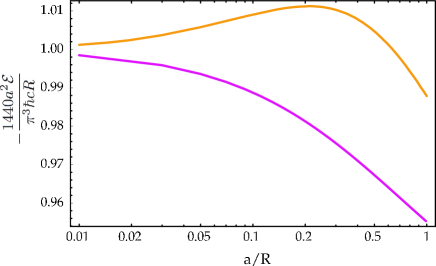
Figure 12: Comparison between the optical approximation (upper curve) and the “semiclassical” approximation of Schaden and Spruch (lower curve) for the sphere and plane. The scaled Casimir energy is plotted versus $a/R$. For the optical approximation, the sum of the first four reflections has been rescaled to go to unity as $a\to 0$. It is possible to show that in the limit $a/R\gg 1$ the optical approximation and Schaden and Spruch’s formula agree (in the figure they both tend to $90/\pi^{4}=0.92...$). The most notable and relevant discrepancies are in the derivative at small $a/R$.

In the cases in which these problems can be avoided, like a sphere of fixed radius in front of a plane, and for $a/R\ll 1$ the semiclassical approximation à la Schaden and Spruch provides quite a good approximation (see figure) since in the expansion (III.35) the stationary phase approximation gives a much larger contribution than the integration by parts terms. A much stronger disagreement has to be expected if the sphere gets substituted by a plate of width $w$ bent with a curvature of order $R\gg w$. Indeed the method of Ref. SandS differs dramatically from the optical approximation for the case of a hyperboloidSSJ . This is not a diffraction effect but rather a ‘precocious’ breakdown of the semiclassical approximation which is cured by a uniform approximation of the kind we have described.

IV Conclusions

We have proposed a new method for calculating approximately Casimir energies between conductors in generic geometries. We use a stationary phase approximation imported from studies of wave optics that we have therefore named the “optical approximation”. In this paper, the first of the series, we have outlined the derivation and applied it to three examples: the canonical example of parallel plates; the experimentally relevant situation of a sphere facing a plane; and the “Casimir pendulum”, i.e. a conducting plate free to oscillate above an infinite plate, where the calculations can be performed analytically. In all of the above examples (except for parallel plates, where our result coincides with Casimir solution) the agreement with the Proximity Force Approximation is only to the leading order in the small distances expansion. The first order correction is found to be different. This is of particular importance in the example of the sphere and the plane because the first order correction in $a/R$ ($a$ is the distance sphere-plate and $R$ is the radius of the sphere) will soon be measured by new precision experiments MPprivate . The optical approximation turns the Casimir sum over modes into a sum over topologically different paths, and from this point of view can be compared with the Poisson summation formula, which has proved useful to derive semiclassical uniform expansions for very diverse problems Berry72 ; Berry76 . In the case of the Casimir energy, replacing the usual highly divergent sum over modes by a sum over topologically distinct optical paths has two, very significant advantages: first, we have been able to show that the divergences in the Casimir energy are contained in contributions of very simple, one-reflection paths and can be easily and unequivocally regulated and discarded; and second, the convergence of the sum over paths is very rapid. Instead of requiring an infinite number of eigenvalues with exquisite precision one needs but a few path contributions, calculated with little numerical effort, to give a very good approximation to the Casimir energy for important geometries. “Semiclassical” methods have been used previously in the study of Casimir effects and the connection between closed orbits and the finite part of the Casimir energy has been pointed out many times Fulling . Our analysis shares with those the idea of shifting attention to approximations and to properties of the Helmholtz propagator. We have shown however that in order to obtain a correct low curvature approximation one has to use a uniform approximation of the kind we proposed here. There is plenty of room to improve the approximation presented here, especially when the connection with Balian and Bloch’s multiple reflection expansion is made explicit. In particular it is intriguing that the Casimir energy for the sphere-plane problem is a well-defined problem in a single variable, namely $x=a/R$ whose limiting values for $x\ll 1$ and $x\gg 1$ are famous CasimirPolder ; BalianDuplantier . One can hope that an analytic solution or an approximation good for the entire range $x$-values should be relatively easy to find. On the contrary it is an incredibly difficult problem and nobody has succeeded in finding such an exact solution or a valid approximation. In the next paper we will show how the same approximation for the propagator can give useful expansions for local operators like the energy-momentum tensor, which allows us to calculate the pressure the energy density and other properties of the constrained field. We will show what our approach has to say about the thermal corrections, which are a controversial matter in Casimir physics. In another paper of the series we will also perform the same analysis for a field of spin 1/2 and and for the electromagnetic field.

V Acknowledgements

A. S. would like to thank M. V. Berry and all the Theory Group of H. H. Wills Laboratories at Bristol University, where part of this work has been done, for their hospitality and for many discussions. We would like to thank P. Facchi, S. Fulling, I. Klitch, L. Levitov, L. Schulman and F. Wilczek, for early discussions. We are grateful to H. Gies for correspondence and numerical values of ref.Gies03 , to M. Schaden and L. Spruch for correspondence and conversations regarding ref.SandS and to G. Klimchitskaya and V. Mostepanenko for discussions. This work is supported in part by the U.S. Department of Energy (D.O.E.) under cooperative research agreement #DF-FC02-94ER40818. A. S. is partially supported by INFN.

References

- (1) S. K. Lamoreaux, Phys. Rev. Lett. 78, 5 (1997); M. Bordag, U. Mohideen and V. M. Mostepanenko, Phys. Rept. 353, 1 (2001) [arXiv:quant-ph/0106045]; G. Bressi, G. Carugno, R. Onofrio and G. Ruoso, Phys. Rev. Lett. 88, 041804 (2002).
- (2) H. B. G. Casimir, Proc. K. Ned. Akad. Wet. 51, 793 (1948).
- (3) R. Golestanian and M. Kardar, Phys. Rev. A 58, 1713 (1998) [arXiv:quant-ph/9802017].
- (4) H. Gies, K. Langfeld and L. Moyaerts, JHEP 0306, 018 (2003) [arXiv:hep-th/0303264].
- (5) B. V. Derjagin, Kolloid Z. 69 155 (1934), B. V. Derjagin, I. I. Abriksova, and E. M. Lifshitz, Sov. Phys. JETP 3, 819 (1957); For a modern discussion of the Proximity Force Theorem, see J. Blocki and W. J. Swiatecki, Annals Phys. 132, 53 (1981).
- (6) R. L. Jaffe and A. Scardicchio, Phys. Rev. Lett. 92, 070402 (2004) [arXiv:quant-ph/0310194].
- (7) M. Born and E. Wolf, Principles of Optics, Cambridge Univ. Press. (1980).
- (8) M. Kline and I. W. Kay, Electromagnetic theory and geometrical optics, Interscience, N.Y. (1965).
- (9) O. Schroeder, A. Scardicchio, and R. L. Jaffe, in preparation.
- (10) N. Graham, R. L. Jaffe, V. Khemani, M. Quandt, M. Scandurra and H. Weigel, Nucl. Phys. B 645, 49 (2002) [arXiv:hep-th/0207120].
- (11) M. Schaden and L. Spruch, Phys. Rev. A 58, 935 (1998); Phys. Rev. Lett. 84, 459 (2000).
- (12) L. S. Brown and G. J. Macay, Phys. Rev. 184, 1272 (1969).
- (13) D. Deutsch and P. Candelas, Phys. Rev. D 20, 3063 (1979).
- (14) R. P. Feynman, Lectures on Physics, Addison Wesley, (1970).
- (15) J. B. Keller, J. Opt. Soc. Am. 52, 116 (1962); J. B. Keller, in Calculus of Variations and its Application (Am. Math. Soc., Providence, 1958), p. 27; B. R. Levy and J. B. Keller, Commun. Pure Appl. Math. XII, 159 (1959); B.R. Levy and J. B. Keller, Can. J. Phys. 38, 128 (1960).
- (16) M. C. Gutzwiller, J. Math. Phys.12, 343 (1971); Chaos in Classical and Quantum Mechanics, Springer, Berlin (1990).
- (17) S. A. Fulling, J. Phys. A 35, 4049 (2002).
- (18) See, for example, V. M. Mostepanenko and N. N. Trunov, Casmir Effects and Its Applications, Oxford University press, (1997).
- (19) J. S. Dowker and G. Kennedy, J. Phys. A 11, 895, (1978).
- (20) For a discussion, see Appendix A in Ref. Graham:2002xq .
- (21) N. Graham, R. L. Jaffe, V. Khemani, M. Quandt, O. Schroeder and H. Weigel, Nucl. Phys. B 677, 379 (2004) [arXiv:hep-th/0309130].
- (22) R. P. Feynman and A. R. Hibbs, Quantum Mechanics and Path Integrals, McGraw-Hill, (1965).
- (23) M. V. Berry and K. E. Mount, Reps. Prog. Phys 35, 315 (1972).
- (24) Y. A. Kravtsov, Sov. Phys.-Acoust. 14, 1 (1968).
- (25) L. S. Schulman, Techniques and Applications of Path Integration, John Wiley & Sons; (1981).
- (26) M. Born and E. Wolf, Principles of Optics, Cambridge University Press; 7th edition (1999).
- (27) J. H. Hannay and A. Thain, [arXiv:physics/0303093] (2003).
- (28) R. S. Decca, E. Fischbach, G. L. Klimchitskaya, D. E. Krause, D. L. Lopez and V. M. Mostepanenko, Phys. Rev. D 68, 116003 (2003) [arXiv:hep-ph/0310157].
- (29) G. L. Klimchitskaya and V. M. Mostepanenko, private communications.
- (30) T. Poston and I. Stewart, Catastrophe Theory And Its Applications, Dover, NY, (1996).
- (31) M. V. Berry and C. Upstill, Progress in Optics XVIII, 257 (1980).
- (32) R. Balian and C. Bloch, Annals Phys. 69, 401 (1970); 63, 592 (1971); 69, 76 (1972).
- (33) R. Balian and B. Duplantier, Annals Phys. 104, 300 (1977); 112, 165 (1978).
- (34) H. Feshbach, Theoretical Nuclear Physics, Nuclear Reactions, Wiley-Interscience; (1993).
- (35) F. D. Mazzitelli, M. J. Sanchez, N. N. Scoccola and J. von Stecher, Phys. Rev. A 67, 013807 (2003) [arXiv:quant-ph/0209097].
- (36) N. Bleistein and R. A. Handelsman, Asymptotic Expansions of Integrals, Dover, NY (1975).
- (37) S. C. Creagh and R. L. Littlejohn, Phys. Rev. A 44 836 (1991).
- (38) S. C. Creagh, Annals Phys. 248 60 (1996).
- (39) M. V. Berry, M. Tabor, Proc. Roy. Soc. Lond, A349, 101 (1976).
- (40) H. B. G. Casimir and D. Polder, Phys. Rev. 73, 360 (1948).
- (41) M. Schaden, private communication.
- (42) M. Schaden and L. Spruch, [arXiv:cond-mat/0304290] (2003).