Photon Statistics of a Non-Stationary Periodically Driven Single-Photon Source

Abstract

We investigate the photon statistics of a single-photon source that operates under non-stationary conditions. The photons are emitted by shining a periodic sequence of laser pulses on single atoms falling randomly through a high-finesse optical cavity. Strong antibunching is found in the intensity correlation of the emitted light, demonstrating that a single atom emits photons one-by-one. However, the number of atoms interacting with the cavity follows a Poissonian statistics so that, on average, no sub-Poissonian photon statistics is obtained, unless the measurement is conditioned on the presence of single atoms.

1 Introduction

Worldwide, major efforts are made to realise systems for the storage of individual quantum bits (qubits) and to conditionally couple different qubits for the processing of quantum information [1]. Ultra-cold trapped neutral atoms or ions are ideal quantum memories that store qubits in long-lived states, while single photons may act as flying qubits that allow for linear optical quantum computing [2]. On the route to a scalable quantum-computing network, interconverting these stationary and flying qubits is essential [3]. One way to accomplish such an interface is by an adiabatic coupling between a single atom and a single photon in an optical cavity [4, 5].

The present work focusses on the properties of a coupled atom-cavity system which is operated as a single-photon emitter [6, 7, 8, 9]. In contrast to other methods of Fock-state preparation in the microwave regime [10, 11], where the photons remain trapped inside the cavity, our scheme allows one to emit single optical photons on demand into a well-defined mode of the radiation field outside the cavity[12, 13]. However, in contrast to many other single-photon sources, like solid-state systems [14, 15, 16], our source operates under non-stationary conditions, because atoms enter and leave the cavity randomly. Only during the presence of a single atom, the atom-cavity system is acting as a single-photon emitter. No photons are generated without atoms, and if more than one atom is present, the number of simultaneously emitted photons might exceed one. These circumstances have a significant impact on the photon statistics of the emitted light [17, 18], which is analysed here in detail.

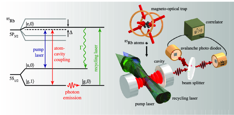
Figure 1: Scheme of the experiment. left: Relevant levels and transitions in ⁸⁵Rb. The atomic states labelled $\left|u\right\rangle$, $\left|e\right\rangle$ and $\left|g\right\rangle$ are involved in the Raman process, and the states $\left|0\right\rangle$ and $\left|1\right\rangle$ denote the photon number in the cavity. right: Setup: A cloud of atoms is released from a magneto-optical trap and falls through a cavity $20\,$cm below in about $8\,$ms with a velocity of $2\,$m/s. The interaction time of each atom in the cloud with the TEM₀₀ mode of the cavity amounts to about $20\,\mu$s. The pump and recycling lasers are collinear and overlap with the cavity mode. The light emitted from the cavity is registered by a pair of photo diodes in Hanbury-Brown & Twiss configuration in order to analyse the photon statistics.

2 Single Photons from a Cavity-QED System

Figure 1 illustrates the basic scheme of the process. A dilute cloud of ⁸⁵Rb atoms, prepared in state $|u\rangle\equiv|5S_{1/2}(F=3)\rangle$, is released from a magneto-optical trap (MOT) and falls with a velocity of $2\,$m/s through a 1 mm long optical cavity of finesse $F=60000$. The density of the cloud, and therefore the average number of atoms simultaneously interacting with the TEM₀₀ mode of the cavity, is freely adjustable. The cavity is near resonant with the transition between the $|5S_{1/2}(F=2)\rangle$ hyperfine state of the electronic ground state and the electronically excited $|5P_{3/2}(F=3)\rangle$ state, labelled $|g\rangle$ and $|e\rangle$, respectively. Initially, the cavity is empty, so that the state of the coupled atom-cavity system can only move within the Hilbert space spanned by the product states $|u,0\rangle$, $|e,0\rangle$, $|g,1\rangle$ and $|g,0\rangle$, with $|0\rangle$ and $|1\rangle$ denoting the relevant photon number states of the cavity. The dynamics of this system is determined by $(g_{max},\kappa,\gamma_{\perp},\Delta)/2\pi=(2.5,1.25,3.0,-20.0)\,$MHz, where $g_{max}$ is the cavity-induced coupling between states $|e,0\rangle$ and $|g,1\rangle$ for an atom optimally coupled to the cavity, and $\kappa$ and $\gamma_{\perp}$ are the field and polarisation decay rates of the cavity and the atom, respectively, and $\Delta$ is the detuning of the cavity from the atomic transition. One mirror has a larger transmission coefficient than the other so that photons leave the cavity through this output coupler with a probability of 90%. While an atom interacts with the cavity, it experiences a sequence of laser pulses that alternate between triggering single-photon emissions and recycling the atom to state $|u\rangle$: The $2\,\mu$s long pump pulses are detuned by $\Delta$ from the $|u\rangle\leftrightarrow|e\rangle$ transition, so that they adiabatically drive a stimulated Raman transition (STIRAP) [19, 8] from $|u,0\rangle$ to $|g,1\rangle$ with a Rabi frequency that increases linearly from 0 to $\Omega_{max}/2\pi=8.0\,$MHz. This Raman transition goes hand-in-hand with a photon emission. Once the photon is emitted, the system reaches $|g,0\rangle$, which is not coupled to the single-excitation manifold, $\{|u,0\rangle,|e,0\rangle,|g,1\rangle\}$, and therefore cannot be re-excited. This limits the number of photons per pump pulse and atom to one.

To emit a sequence of photons from one-and-the-same atom, the system is transferred back to $\left|u,0\right\rangle$ after each emission. To do so, we apply $2\,\mu$s long recycling laser pulses that hit the atom between consecutive pump pulses. The recycling pulses are resonant with the $\left|g\right\rangle\leftrightarrow\left|e\right\rangle$ transition and excite the atom to state $\left|e\right\rangle$. From there, it decays spontaneously to the initial state, $\left|u\right\rangle$. In this way, an atom that resides in the cavity can emit a sequence of single-photon pulses. For each experimental cycle, these photons are recorded using two avalanche photo diodes with 50% quantum efficiency, which are placed at the output ports of a beam splitter.

3 Photon Statistics

The two photo diodes constitute a Hanbury-Brown & Twiss setup [20] which we use to measure the normalised intensity correlation of the photon stream emitted from the cavity,

$$g^{(2)}(\tau)=\frac{\langle I_{1}(t)I_{2}(t+\tau)\rangle}{\langle I_{1}(t)\rangle\langle I_{2}(t)\rangle},$$ (1)

where $I_{n}(t)$ is the count rate recorded by detector $n=1,2$. If $\bar{I}$ denotes the mean count rate recorded by each detector and $\bar{I}_{N}$ is the mean noise-count rate, the mean rate of photon-counts reads $\bar{I}_{P}=\bar{I}-\bar{I}_{N}$. This allows to estimate two of the three following contributions to the correlation function:

• Correlations between a noise count and either a real photon or another noise count are randomly distributed and occur with a probability proportional to $\bar{I}^{2}_{N}+\bar{I}_{P}\bar{I}_{N}+\bar{I}_{N}\bar{I}_{P}=\bar{I}^{2}-\bar{I}_{P}^{2}$. Therefore these correlations lead to a constant background contribution,

  $$g^{(2)}_{N}=\frac{\bar{I}^{2}-\bar{I}_{P}^{2}}{\bar{I}^{2}}=1-\frac{\bar{I}_{P}^{2}}{\bar{I}^{2}},$$ (2)

  to the normalised correlation function.

• Correlations between photons that stem from different atoms lead to a modulation of $g^{(2)}(\tau)$, since the periodicity of the pump laser leads to a modulation of the photon emission probability. The pump intervals have the same duration as the recycling intervals, and the probability for photon emissions during recycling is close to zero. This increases the average rate of photons emitted during pumping to $2\bar{I}_{P}$, so that photon-photon correlations between pump pulses are found with a probability proportional to $(2\bar{I}_{P})^{2}$, while the probability to get photon correlations between pump- and recycling intervals is vanishingly small. The average normalised contribution of photon-photon correlations to $g^{(2)}$ therefore oscillates between

  $$g^{(2)}_{P,min}=0\qquad\mbox{and}\qquad g^{(2)}_{P,max}=\frac{1}{2}\frac{(2\bar{I}_{P})^{2}}{\bar{I}^{2}}=2\frac{\bar{I}_{P}^{2}}{\bar{I}^{2}}.$$ (3)

  In order to obtain this simple estimation, we use the factor $\frac{1}{2}$ in $g^{(2)}_{P,max}$ to take into account that photons are emitted only during pump pulses, which are active half of the time, and we neglect any time-dependence of $I_{P}$ within the pump pulses. In the experiment, however, $I_{P}$ varies with time, which causes small deviations from the estimated values, as further discussed below.

  

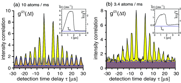
  Figure 2: Unconditional photon statistics of the emitted light: Intensity correlation, $g^{(2)}(\Delta t)$, with different-atom (hatched) and noise (cross-hatched) contributions. For correlation times larger than the atom-cavity interaction time, only these contributions persist. They are calculated by a convolution of the respective pulse-averaged count rates, $\tilde{I}(t)$, which are shown in the two insets. (a) High atom flux, averaged over 4997 experimental cycles (loading and releasing of the atom cloud) with a total number of 151089 photon counts. (b) Low atom flux, averaged over 15000 experimental cycles with a total number of 184868 photon counts.

• Correlations between photons emitted from one-and-the-same atom are, of course, most interesting. They cannot be estimated from the average count rates, $\bar{I}$ and $\bar{I}_{N}$. However, due to the limited atom-cavity interaction time, $\tau_{int}$, it is clear that they only contribute to $g^{(2)}(\tau)$ in the time interval $[-\tau_{int}\ldots\tau_{int}]$, and therefore this contribution can be distinguished from (a) and (b) as explained below.

Figure 2(a and b), obtained for a different flux of atoms, shows that the three contributions above are easily identified in the measured correlation function. Due to the limited atom-cavity interaction time, all correlations with $|\tau|\gg\tau_{int}$ either belong to category (a) or (b). The oscillatory behaviour of $g^{(2)}(\tau)$ in this regime stems from photons emitted by different atoms, whereas the time-independent pedestal is mainly caused by correlations involving noise counts. These two contributions are indicated as hatched and cross-hatched areas, respectively. They were calculated by a convolution of the pulse-averaged count rate, $\tilde{I}(t)=\frac{1}{N}\sum_{n=1}^{N}I(t+n\tau_{period})$, with a total number of $N$ recorded pump&recycle intervals of duration $\tau_{period}=4\,\mu$s. This gives an oscillation of the intensity correlation function between $g^{(2)}_{C,min}$ and $g^{(2)}_{C,max}$.

These two values of $g^{(2)}$ can also be estimated from the mean count rates, $\bar{I}$ and $\bar{I}_{N}$. This estimation predicts an oscillation of $g^{(2)}$ with the periodicity of the applied sequence between the two extrema $g^{(2)}_{E,min}=1-\frac{\bar{I}_{P}^{2}}{\bar{I}^{2}}$ and $g^{(2)}_{E,max}=1+\frac{\bar{I}_{P}^{2}}{\bar{I}^{2}}$. For the data underlying Fig. 2, we obtain the following result:

	high atom flux, Fig. 2(a)	low atom flux, Fig. 2(b)
$\bar{I}$	1976 s-1	783 s-1
$\bar{I}_{N}$	446 s-1	446 s-1
$\bar{I}_{P}=\bar{I}-\bar{I}_{N}$	1530 s-1	337 s-1
$g^{(2)}_{E,min}\ldots g^{(2)}_{E,max}$	$0.40\ldots 1.60$	$0.81\ldots 1.19$
$g^{(2)}_{C,min}\ldots g^{(2)}_{C,max}$	$0.46\ldots 1.82$	$0.91\ldots 1.13$

As mentioned above, the estimated values deviate slightly from the values obtained from the convolution of the pulse-averaged count rate. This was expected due to the simplified model our estimation is based on. Note that contributions (a) and (b) persist also in the regime $|\tau|<\tau_{int}$, since the atoms have a Poissonian distribution. Obviously, the excess signal observed here belongs to category (c), i.e. it reflects the single-atom contribution to the correlation signal. Most remarkably, no excess signal is found around $\tau=0$, i.e. all correlations registered during one-and-the-same pump pulse either involve noise counts or photons from different atoms. Correlations between photons that stem from one-and-the-same atom (c) are only found between different pump pulses. Moreover, antibunching with $g^{(2)}(0)<g^{(2)}(\tau=n\tau_{period})$, $n=\pm 1,\pm 2,\ldots$, is observed. This effect cannot be observed for a classical light source, where the Cauchy-Schwartz inequality predicts that $g^{(2)}(0)\geq g^{(2)}(\tau)$ [21]. Therefore the observation of antibunching indicates that a single atom emits photons one-by-one.

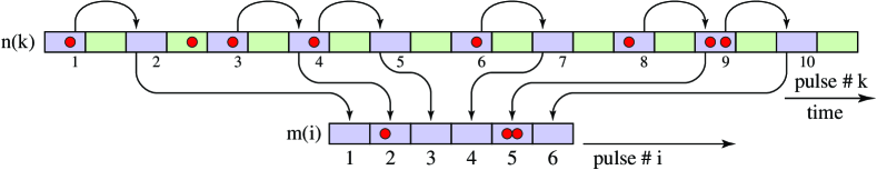
Figure 3: Conditioning on the presence of atoms (schematic): All events (red bullets) are first recorded as a function of time. If photons are detected in a time interval where the pump laser is active (blue intervals), we assume that an atom is present and take the following pump-laser interval into account. Events recorded during recycling (green intervals) are ignored. The pump-laser intervals selected this way form a new set of data, which is then used to calculate the intensity correlation function.

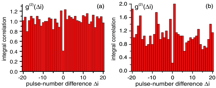
Figure 4: Conditional photon statistics: A sub-Poissonian photon statistics is found in the pulse-to-pulse photon correlation, $g^{(2)}{(\Delta i)}$, conditioned on the presence of atoms in the cavity. Data are shown for high atom flux (a) and low atom flux (b) as stated in Fig. 2.

In case of a stationary single-photon source, the non-classicality of the emitted radiation would lead to a sub-Poissonian photon statistics with $g^{(2)}(0)<1$. In the present case, however, atoms arrive randomly in the cavity, and the Poissonian atom statistics leads to $g^{(2)}(0)>1$. An a-priori knowledge on the presence of an atom is therefore needed to operate the apparatus as a single-photon emitter. Indeed, if the statistical analysis of the emitted photon stream is restricted to time intervals where the presence of an atom in the cavity is assured with very high probability, a sub-Poissonian photon statistics is found. Figure 3 illustrates the conditioning scheme: To detect an atom, we rely on the fact that photons are only emitted while an atom resides in the cavity. Thus a photon that is detected during a pump pulse signals the presence of an atom with probability $p_{atom}=\bar{n}_{P}/(\bar{n}_{P}+\bar{n}_{N})$, where $\bar{n}_{N}=2\bar{I}_{N}\times\tau_{P}$ is the mean number of noise counts per pump pulse counted by both detectors, and $\bar{n}_{P}=2\int_{0}^{\tau_{P}}(\tilde{I}(t)-\bar{I}_{N})dt$ is the mean number of detected photons per pulse, with $\tau_{P}=2\,\mu$s being the pulse duration. For the data underlying Fig. 2, we obtain $(\bar{n}_{P},\bar{n}_{N},p_{atom})=(11.6\times 10^{-3},1.8\times 10^{-3},87\%)$ and $(2.3\times 10^{-3},1.8\times 10^{-3},56\%)$ for high and low atom flux, respectively. The small value of $\bar{n}_{P}$ is due to the fact that the cavity contains no atom most of the time. But once an atom is detected, it moves only 1/5 of the cavity waist until the next pump pulse arrives. We can therefore safely assume that the atom still resides in the cavity at that moment. In the statistical analysis of the light emitted from the system, we now include only the time interval corresponding to this next pump pulse. This is accomplished by first denoting the numbers, $k_{1}\ldots k_{M}$, of the $M$ pump intervals with $n(k_{i})>0$, where $n(k_{i})$ denotes the number of photons detected in the $k_{i}$th interval. The time intervals of the adjacent pump pulses then form the new stream of selected data, where the number of photons counted with detector 1 and 2, respectively, is given by $m_{1,2}(i)=n_{1,2}(k_{i}+1)$. From this, the conditioned correlation function,

$$g^{(2)}(\Delta i)=\frac{1}{M}\sum_{i=1}^{M}\frac{m_{1}(i)m_{2}(i+\Delta i)}{\bar{m}_{1}\bar{m}_{2}},$$ (4)

shown in Fig. 4, is calculated. In case of a small average atom number, see Fig. 4(b), conditioning yields $g^{(2)}(\Delta i=0)=0.25(11)$, which is well below one. If the atom flux is increased, Fig. 4(a), one obtains $g^{(2)}(\Delta i=0)=0.41(6)$. Obviously the larger value is due to the fact that the probability of having more than one atom interacting with the cavity is not negligible. Nevertheless, the photon statistics conditioned on the presence of atoms is sub-Poissonian in both cases, which is demonstrating a noise reduction below the shot-noise level. Note that the errors in $g^{(2)}(\Delta i)$ are derived from the standard deviations, $\sigma_{\Delta i}=\sqrt{n_{e}(\Delta i)}$, where $n_{e}(\Delta i)$ denotes the number of events that constitute $g^{(2)}(\Delta i)$ prior to normalisation. We count $n_{e}(\Delta i=0)=5\pm 2.2$ and $53\pm 7.3$ events, whereas for $\Delta i\neq 0$, we count, on average, $\bar{n}_{e}=21$ and 130 events with $\sigma_{\Delta i\neq 0}=4.6$ and 11.4, which yields $\bar{g}^{(2)}(\Delta i\neq 0)=1.00(20)$ and 1.00(9), for low and high atom flux, respectively. The fluctuations of $g^{(2)}(\Delta i\neq 0)$ in Fig. 4 are well explained by this shot noise.

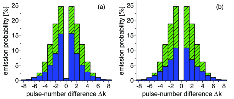
Figure 5: Photon emission probability, conditioned on a photon detection at $\Delta k=0$. The theoretical expectation values are represented by the green dashed bars, while the experimentally found probabilities are indicated by the solid blue bars. Data are shown for high atom flux (a) and low atom flux (b) as stated in Fig. 2. The decrease of the experimentally observed probabilities in (b) as compared to (a) is attributed to a small misalignment of the setup for low atom flux.

From the recorded stream of events, we can also characterise the efficiency of the photon source by evaluating the probability for the conditional emission of photons during the pump pulses that follow the detection of an atom by a first photodetection (Fig. 5). The evaluation must encompass a correction for detector effects like noise counts and reduced quantum efficiencies. Hence, we take into account that a single photodetection actually signals the presence of an atom only with probability $p_{atom}$, and we also consider that the following photons are detected with an overall quantum efficiency of $\eta=0.36$ (photo diodes and spatial filtering). We then use the $M$ pump intervals with $n(k_{i})>0$ as starting points to calculate the average photo-emission probabilities during the neighbouring pulses,

$$\bar{p}(\Delta k)=\frac{1}{\eta\ p_{atom}}\frac{1}{M}\sum_{i=1}^{M}\left[n(k_{i}+\Delta k)-\bar{n}_{N}-\bar{n}_{P}-\delta_{\Delta k,0}\right].$$ (5)

Here, $n(k)=n_{1}(k)+n_{2}(k)$ is the total number of events counted by both detectors during the $k$th pump pulse. The mean number of noise counts per pulse, $\bar{n}_{N}$, and the mean number of photons per pulse, $\bar{n}_{P}$, are subtracted from each count number to ensure that only photons emitted from one-and-the same atom are considered. We also correct for false triggers, i.e. noise counts signalling atoms which are not present, and the quantum efficiency of the photodetection. Note that the $M$ conditioning photodetections are not counted twice, since we subtract $\delta_{\Delta k,0}$ from the calculated probabilities, with $\delta_{i,j}=1$ for $i=j$ and $\delta_{i,j}=0$ otherwise. Obviously, the probabilities for subsequent photon emissions decrease from pulse-to-pulse, since the efficiency of the photon generation depends on the location of the moving atom. It is highest in an anti-node on the cavity axis and decreases if the atom moves away from this point. A simulation of the process, based on a numerical solution of the master equation, allows the calculation of the expected photon-emission probabilities averaged over the random trajectories of the atoms travelling through the cavity. This leads to the same qualitative results, but the experimentally determined emission probabilities are smaller than the expected ones. We attribute this discrepancy to the random distribution of the atom among its magnetic sublevels after recycling, which reduces the overall efficiency of the photon generation. In our numerical simulation, this has been neglected. A more rigourous analysis is beyond the scope of this paper. Another significant feature of the numerical analysis is the prediction of a single-photon generation efficiency of $61.6\%$ for an atom which is optimally coupled to the cavity. Therefore we expect that the present scheme is able to produce single photons in a highly efficient way provided the atom is hold at rest by, e.g., a dipole-force trap [22, 23, 24].

4 Summary

We have statistically analysed the photon stream emitted from a strongly coupled atom-cavity system in response to laser pulses that adiabatically drive Raman transitions between two atomic states. The laser pulses excite one branch of the transition, while the vacuum field of the cavity stimulates the other branch. The cavity operates as a non-stationary single-photon source, since the atoms enter and leave the mode volume randomly, with a maximum number of about 7 successive photon emissions per atom. Without any a-priori knowledge on the state of the system, antibunching is observed, which indicates that a single atom emits photons one-by-one. Furthermore, a preselection has been applied to restrict the analysis to time intervals where the presence of an atom is assured. This gives a sub-Poissonian photon statistics with $g^{(2)}(0)<1$. Our setup therefore operates as a deterministic single-photon emitter, although the atom statistics is Poissonian.

References

References

- [1] D. Bouwmeester, A. Ekert, and A. Zeilinger, editors. The Physics of Quantum Information. Springer, Berlin, 2000.
- [2] E. Knill, R. Laflamme, and G. J. Milburn. A scheme for efficient quantum computing with linear optics. Nature, 409:46–52, 2001.
- [3] D. P. DiVincenzo. The physical implementation of quantum computation. Fortschr. Phys., 48:771, 2000.
- [4] S. van Enk, J. I. Cirac, P. Zoller, H. J. Kimble, and H. Mabuchi. Quantum state transfer in a quantum network: A quantum optical implementation. J. Mod. Opt., 44:1727, 1997.
- [5] J. I. Cirac, P. Zoller, H. J. Kimble, and H. Mabuchi. Quantum state transfer and entanglement distribution among distant nodes in a quantum network. Phys. Rev. Lett., 78:3221–3224, 1997.
- [6] A. Kuhn, M. Hennrich, T. Bondo, and G. Rempe. Controlled generation of single photons from a strongly coupled atom-cavity system. Appl. Phys. B, 69:373–377, 1999.
- [7] A. Kuhn and G. Rempe. Optical cavity qed: Fundamentals and application as a single-photon light source. In F. De Martini and C. Monroe, editors, Experimental Quantum Computation and Information, volume 148, pages 37–66. IOS-Press, 2002.
- [8] M. Hennrich, A. Kuhn, and G. Rempe. Counter-intuitive vacuum-stimulated Raman scattering. J. Mod. Opt., 50:936–942, 2003.
- [9] A. Kuhn, M. Hennrich, and G. Rempe. Strongly-coupled atom-cavity systems. In T. Beth and G. Leuchs, editors, Quantum Information Processing, pages 182–195. Wiley-VCH, Berlin, 2003.
- [10] X. Maître, E. Hagley, G. Nogues, C. Wunderlich, P. Goy, M. Brune, J.-M. Raimond, and S. Haroche. Quantum memory with a single photon in a cavity. Phys. Rev. Lett., 79:769–772, 1997.
- [11] S. Brattke, B. T. H. Varcoe, and H. Walther. Generation of photon number states on demand via cavity quantum electrodynamics. Phys. Rev. Lett., 86:3534–3537, 2001.
- [12] M. Hennrich, T. Legero, A. Kuhn, and G. Rempe. Vacuum-stimulated Raman scattering based on adiabatic passage in a high-finesse optical cavity. Phys. Rev. Lett., 85:4872–4875, 2000.
- [13] A. Kuhn, M. Hennrich, and G. Rempe. Deterministic single-photon source for distributed quantum networking. Phys. Rev. Lett., 89:067901, 2002.
- [14] C. Kurtsiefer, S. Mayer, P. Zarda, and H. Weinfurter. Stable solid-state source of single photons. Phys. Rev. Lett., 85:290–293, 2000.
- [15] A. Beveratos, R. Brouri, T. Gacoin, J.-P. Poizat, and P. Grangier. Nonclassical radiation from diamond nanocrystals. Phys. Rev. A, 64:061802, 2001.
- [16] C. Santori, D. Fattal, J. Vučković, G. S. Solomon, and Y. Yamamoto. Indistinguishable photons from a single-photon device. Nature, 419:594–597, 2002.
- [17] H. J. Kimble. Comment on “Deterministic single-photon source for distributed quantum networking”. Phys. Rev. Lett., 90:249801, 2003.
- [18] A. Kuhn, M. Hennrich, and G. Rempe. A reply to the comment by Harry J. Kimble. Phys. Rev. Lett., 90:249802, 2003.
- [19] N. V. Vitanov, M. Fleischhauer, B. W. Shore, and K. Bergmann. Coherent manipulation of atoms and molecules by sequential laser pulses. Adv. At. Mol. Opt. Phys., 46:55–190, 2001.
- [20] R. Hanbury Brown and R. Q. Twiss. A test of a new type of stellar interferometer on Sirius. Nature, 178:1046–1448, 1956.
- [21] D. F. Walls and G. J. Milburn. Quantum Optics. Springer, Berlin, 1994.
- [22] S. Kuhr, W. Alt, D. Schrader, M. Müller, V. Gomer, and D. Meschede. Deterministic delivery of a single atom. Science, 293:278–280, 2001.
- [23] J. A. Sauer, K. M. Fortier, M. SW. Chang, C. D. Hamley, and M. S. Chapman. Cavity qed with optically transported atoms. quant-ph/0309052, 2003.
- [24] J. McKeever, A. Boca, A. D. Boozer, J. R. Buck, and H. J. Kimble. Experimental realization of a one-atom laser in the regime of strong coupling. Nature, 425:268–270, 2003.