Degaussification of twin-beam and nonlocality in the phase space

Abstract

We show that inconclusive photon subtraction (IPS) on twin-beam produces non-Gaussian states that violate Bell’s inequality in the phase-space. The violation is larger than for the twin-beam itself irrespective of the IPS quantum efficiency. The explicit expression of IPS map is given both for the density matrix and the Wigner function representations.

I Introduction

The twin-beam state (TWB) of two modes of radiation can be expressed in the photon number basis as

$$|\Lambda\rangle\rangle_{ab}=\sqrt{1-\lambda^{2}}\,\sum_{n=0}^{\infty}\,\lambda^{n}|n,n\rangle_{ab}\,,$$ (1)

where $\lambda=\tanh(r)$, $r$ being the TWB squeezing parameter. TWB is described by a Gaussian Wigner function

$$W_{r}(\alpha,\beta) = \frac{4}{\pi^{2}}\exp\{-2A(|\alpha|^{2}+|\beta|^{2})$$ (2)

$$\hskip 42.67912pt+2B(\alpha\beta+\overline{\alpha}\overline{\beta})\}\,,$$

with $A\equiv A(r)=\cosh(2r)$ and $B\equiv B(r)=\sinh(2r)$. Since (2) is positive-definite, TWB are not suitable to test nonlocality through homodyne detection. Indeed, the Wigner function itself provides an explicit hidden variable model for homodyne measurements bana ; sanchez . On the other hand, it has been shown bana that TWB exhibits a nonlocal character for parity measurements. This is known as nonlocality in the phase-space since Bell inequalities can be written in terms of the Wigner function, which in turn describes correlations for the joint measurement of displaced parity operators. Overall, the positivity or the negativity of the Wigner function has a rather weak relation to the locality or the nonlocality of quantum correlations.

In Ref. ips:tele we have suggested a conditional measurement scheme on TWB leading to a non Gaussian entangled mixed state, which improves fidelity in the teleportation of coherent states. This process, called inconclusive photon subtraction (IPS), is based on mixing each mode of the TWB with the vacuum in a unbalanced beam splitter and then performing inconclusive photodetection on both modes, i.e. revealing the reflected beams without discriminating the number of the detected photons.

A single mode version of the IPS, mapping squeezed light onto non-Gaussian states, has been recently realized experimentally grangier . Moreover, IPS has been suggested as a feasible method to modify TWB and test nonlocality using homodyne detection sanchez .

In this paper we address IPS as a degaussification map for TWB, give its explicit expression for the density matrix and the Wigner function, and investigate the nonlocality of the resulting state in the phase-space.

The paper is structured as follows. In Section II we review nonlocality in the phase-space, i.e. Wigner function Bell’s inequality based on measuring the displaced parity operator on two modes of radiation. In Section III we illustrate the IPS process as a degaussification map and calculate the Wigner function of the IPS state. The nonlocality of the IPS state in the phase-space is then analyzed in Section IV, whereas in Section V we discuss nonlocality using homodyne detection, extending the analysis of Ref. sanchez . Section VI closes the paper with some concluding remarks.

II Nonlocality in the phase-space

The displaced parity operator on two modes is defined as

$$\hat{\Pi}(\alpha,\beta) = D_{a}(\alpha)(-1)^{a^{\dagger}a}D_{a}^{\dagger}(\alpha)$$ (3)

$$\hskip 42.67912pt\otimes D_{b}(\beta)(-1)^{b^{\dagger}b}D_{b}^{\dagger}(\beta)\,,$$

where $\alpha,\beta\in{\mathbb{C}}$, $a$ and $b$ are mode operators and $D_{a}(\alpha)=\exp\{\alpha a^{\dagger}-\overline{\alpha}a\}$ and $D_{b}(\beta)$ are single-mode displacement operators. Parity is a dichotomic variable and thus can be used to establish Bell-like inequalities CHSH . Since the two-mode Wigner function $W(\alpha,\beta)$ can be expressed as

$$W(\alpha,\beta)=\frac{4}{\pi^{2}}\,\Pi(\alpha,\beta)\,,$$ (4)

$\Pi(\alpha,\beta)$ being the expectation value of $\hat{\Pi}(\alpha,\beta)$, the violation of these inequalities is also known as nonlocality in the phase-space. The quantity involved in such inequalities can be written as follows

$$\mathcal{B} = \Pi(\alpha_{1},\beta_{1})+\Pi(\alpha_{2},\beta_{1})$$ (5)

$$\hskip 14.22636pt+\Pi(\alpha_{1},\beta_{2})-\Pi(\alpha_{2},\beta_{2})\,,$$

which, for local theories, satisfies the condition $|\mathcal{B}|\leq 2$.

Following Ref. bana , one can choose a particular set of displaced parity operators, arriving at the following combination

$$B(J) = \Pi(0,0)+\Pi(\sqrt{J},0)$$ (6)

$$\hskip 14.22636pt+\Pi(0,-\sqrt{J})-\Pi(\sqrt{J},-\sqrt{J})\,,$$

which only depends on the positive parameter $J$, characterizing the magnitude of the displacement. If we evaluate the quantity (6) in the case of the TWB, we find that it exceeds the upper bound imposed by local theories for a certain region of values $(J,r)$, its maximum being $B\approx 2.19$ bana .

On the other hand, the choice of the parameters leading to Eq. (6) is not the best one, and the violation of the inequality $|\mathcal{B}|\leq 2$ can be enhanced using a different parameterization ferraro . A better result is achieved for

$$C(J) = \Pi(\sqrt{J},-\sqrt{J})+\Pi(-3\sqrt{J},-\sqrt{J})$$ (7)

$$\hskip 14.22636pt+\Pi(\sqrt{J},3\sqrt{J})-\Pi(-3\sqrt{J},3\sqrt{J})\,,$$

which, for the TWB, gives a maximum $C\approx 2.32$, greater than the value $2.19$ obtained in Ref. bana .

In the following Sections we will see that the violation of the inequalities $|B(J)|\leq 2$ and $|C(J)|\leq 2$ can be enhanced by degaussification of the TWB.

III The degaussification process

The degaussification of a TWB can be achieved by subtracting photons from both modes opatr ; coch ; ips:tele . In Ref. ips:tele we referred to this process as to inconclusive photon subtraction and showed that the resulting state, the IPS state $\varrho_{\hbox{\tiny IPS}}$, can be used to enhance the teleportation fidelity of coherent states for a wide range of the experimental parameters.

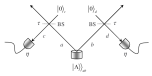
Figure 1: Scheme of the IPS process.

The IPS scheme is sketched in Fig. 1. The two modes, $a$ and $b$, of the TWB are mixed with the vacuum (modes $c$ and $d$, respectively) at two unbalanced beam splitters (BS) with equal transmissivity $\tau=\cos^{2}\phi$; the modes $c$ and $d$ are then revealed by avalanche photodetectors (APD) with equal efficiency $\eta$. APD’s can only discriminate the presence of radiation from the vacuum. The positive operator-valued measure (POVM) $\{\Pi_{0}(\eta),\Pi_{1}(\eta)\}$ of each detector is given by

$${\Pi}_{0}(\eta)=\sum_{j=0}^{\infty}(1-\eta)^{j}|j\rangle\langle j|\>,\quad{\Pi}_{1}(\eta)=\mathbb{I}-{\Pi}_{0}(\eta)\>,$$ (8)

$\eta$ being the quantum efficiency. Overall, the conditional measurement on the modes $c$ and $d$, is described by the POVM (we are assuming the same quantum efficiency for both photodetectors)

$${\Pi}_{00}(\eta) = {\Pi}_{0,c}(\eta)\otimes{\Pi}_{0,d}(\eta)\>,$$ (9)

$${\Pi}_{01}(\eta) = {\Pi}_{0,c}(\eta)\otimes{\Pi}_{1,d}(\eta)\>,$$ (10)

$${\Pi}_{10}(\eta) = {\Pi}_{1,c}(\eta)\otimes{\Pi}_{0,d}(\eta)\>,$$ (11)

$${\Pi}_{11}(\eta) = {\Pi}_{1,c}(\eta)\otimes{\Pi}_{1,d}(\eta)\;.$$ (12)

When the two photodetectors jointly click, the conditioned output state of modes $a$ and $b$ is given by

$$\mathcal{E}(R)=\frac{1}{p_{11}(r,\phi,\eta)}\hbox{Tr}_{cd}\big{[}U_{ac}(\phi)\otimes U_{bd}(\phi)\>R\otimes|0\rangle_{c}{}_{c}\langle 0|\otimes|0\rangle_{d}{}_{d}\langle 0|\>U_{ac}^{{\dagger}}(\phi)\otimes U_{bd}^{{\dagger}}(\phi)\>{\mathbb{I}}_{a}\otimes{\mathbb{I}}_{b}\otimes{\Pi}_{11}(\eta)\big{]}\>,$$ (13)

where $U_{ac}(\phi)=\exp\{-\phi(a^{{\dagger}}c-ac^{{\dagger}})\}$ and $U_{bd}(\phi)$ are the evolution operators of the beam splitters and $R$ the density operator of the two-mode state entering the beam splitters (in our case $R=\varrho_{\hbox{\tiny TWB}}=|\Lambda\rangle\rangle_{ab}{}_{ba}\langle\langle\Lambda|$). The partial trace on modes $c$ and $d$ can be explicitly evaluated, thus arriving at the Kraus decomposition of the IPS map. We have

$$\mathcal{E}(R)=\frac{1}{p_{11}(r,\phi,\eta)}\>\sum_{p,q=1}^{\infty}\>m_{p}(\phi,\eta)\>M_{pq}(\phi)\>R\>M_{pq}^{{\dagger}}(\phi)\>m_{q}(\phi,\eta)\>$$ (14)

with

$$m_{p}(\phi,\eta)={\displaystyle\frac{\tan^{2p}\phi\,\,[1-(1-\eta)^{p}]}{p!}}\,,$$ (15)

and

$$M_{pq}(\phi)=\frac{\mbox{}}{\mbox{}}a^{p}b^{q}\,(\cos\phi)^{a^{\dagger}a+b^{\dagger}b}\,,$$ (16)

and

$$p_{11}(r,\phi,\eta)={\rm Tr}_{ab}[\mathcal{E}(R)]$$ (17)

is the probability of a click in both detectors.

Now, in order to investigate the nonlocality of the state $\varrho_{\hbox{\tiny{IPS}}}=\mathcal{E}(\varrho_{\hbox{\tiny TWB}})$ in the phase-space, we explicitly calculate its Wigner function, which, as one may expect, is no longer Gaussian and positive-definite.

The state entering the two beam splitters is described by the Wigner function

$$W_{r}^{\hbox{\tiny(in)}}(\alpha,\beta,\zeta,\xi)=W_{r}(\alpha,\beta)\,\frac{4}{\pi^{2}}\exp\left\{-2|\zeta|^{2}-2|\xi|^{2}\right\}\,,$$ (18)

where the second factor at the rhs represents the two vacuum states of modes $c$ and $d$. The action of the beam splitters on $W^{\hbox{\tiny(in)}}_{r}$ can be summarized by the following change of variables

$$\alpha \to \alpha\cos\phi+\zeta\sin\phi\,,\quad\zeta\to\zeta\cos\phi-\alpha\sin\phi\,,$$ (19)

$$\beta \to \beta\cos\phi+\xi\sin\phi\,,\quad\xi\to\xi\cos\phi-\beta\sin\phi\,,$$ (20)

and the output state, after the beam splitters, is then given by

$$W_{r,\phi}^{\hbox{\tiny(out)}}(\alpha,\beta,\zeta,\xi) = \frac{4}{\pi^{2}}\,W_{r,\phi}(\alpha,\beta)\,\exp\left\{-a|\xi|^{2}+w\xi+\overline{w}\overline{\xi}\right\}$$ (21)

$$\hskip 14.22636pt\times\exp\left\{-a|\zeta|^{2}+(v+2B\xi\sin^{2}\phi)\zeta+(\overline{v}+2B\overline{\xi}\sin^{2}\phi)\overline{\zeta}\right\}\,,$$

where

$$W_{r,\phi}(\alpha,\beta)=\frac{4}{\pi^{2}}\,\exp\left\{-b(|\alpha|^{2}+|\beta|^{2})+2B\cos^{2}\phi\,(\alpha\beta+\overline{\alpha}\overline{\beta})\right\}$$ (22)

and

$$a \equiv a(r,\phi)=2(A\sin^{2}\phi+\cos^{2}\phi),$$ (23)

$$b \equiv b(r,\phi)=2(A\cos^{2}\phi+\sin^{2}\phi)\,,$$ (24)

$$v \equiv v(r,\phi)=2\cos\phi\,\sin\phi\,[(1-A)\overline{\alpha}+B\beta],$$ (25)

$$w \equiv w(r,\phi)=2\cos\phi\,\sin\phi\,[(1-A)\overline{\beta}+B\alpha]\,.$$ (26)

At this stage conditional on/off detection is performed on modes $c$ and $d$ (see Fig. 1). We are interested in the situation when both the detectors click. The Wigner function of the double click element $\Pi_{11}(\eta)$ of the POVM (see Eq. (12)) is given by ips:tele ; cond:cola

$$W_{\eta}(\zeta,\xi) \equiv W[\Pi_{11}(\eta)](\zeta,\xi)$$ (27)

$$= \frac{1}{\pi^{2}}\{1-Q_{\eta}(\zeta)-Q_{\eta}(\xi)$$

$$\hskip 42.67912pt+Q_{\eta}(\zeta)Q_{\eta}(\xi)\}\,,$$

with

$$Q_{\eta}(z)=\frac{2}{2-\eta}\,\exp\Bigg{\{}-\frac{2\eta}{2-\eta}\,|z|^{2}\Bigg{\}}\,.$$ (28)

Using Eq. (13) and the phase-space expression of trace (for each mode)

$${\rm Tr}[O_{1}O_{2}]=\pi\,\int_{\mathbb{C}}d^{2}z\,W[O_{1}](z)\,W[O_{2}](z)\,,$$ (29)

$O_{1}$ and $O_{2}$ being two operators and $W[O_{1}](z)$ and $W[O_{2}](z)$ their Wigner functions, respectively, the Wigner function of the output state, conditioned to the double click event, is then given by

$$W_{r,\phi,\eta}(\alpha,\beta)=\frac{f_{r,\phi,\eta}(\alpha,\beta)}{p_{11}(r,\phi,\eta)}\,,$$ (30)

where

$$f_{r,\phi,\eta}(\alpha,\beta)=\pi^{2}\,\int_{\mathbb{C}^{2}}d^{2}\zeta\,d^{2}\xi\,\frac{4}{\pi^{2}}\,W_{r,\phi}(\alpha,\beta)\,\sum_{j=1}^{4}\frac{C_{j}(\eta)}{\pi^{2}}\,G_{r,\phi,\eta}^{(j)}(\alpha,\beta,\zeta,\xi)\,,$$ (31)

and $p_{11}(r,\phi,\eta)$ is the double-click probability (17), which can be written as function of $f_{r,\phi,\eta}(\alpha,\beta)$ as follows

$$p_{11}(r,\phi,\eta)=\pi^{2}\,\int_{\mathbb{C}^{2}}d^{2}\alpha\,d^{2}\beta\,f_{r,\phi,\eta}(\alpha,\beta)\,.$$ (32)

The quantity $G_{r,\phi,\eta}^{(j)}(\alpha,\beta,\zeta,\xi)$ appearing in Eq. (31) is

$$G_{r,\phi,\eta}^{(j)}(\alpha,\beta,\zeta,\xi) = \exp\left\{-x_{j}|\zeta|^{2}+(v+2B\xi\sin^{2}\phi)\zeta+(\overline{v}+2B\overline{\xi}\sin^{2}\phi)\overline{\zeta}\right\}$$ (33)

$$\hskip 28.45274pt\times\exp\left\{-y_{j}|\xi|^{2}+w\xi+\overline{w}\overline{\xi}\right\}\,,$$

and the expressions of $C_{j}(\eta)$, $x_{j}\equiv x_{j}(r,\phi,\eta)$ and $y_{j}\equiv y_{j}(r,\phi,\eta)$ are given in Table 1.

Table 1:

$j$	$x_{j}(r,\phi,\eta)$	$y_{j}(r,\phi,\eta)$	$C_{j}(\eta)$
1	$a$	$a$	1
2	$a+\frac{2}{2-\eta}$	$a$	$-\frac{2}{2-\eta}$
3	$a$	$a+\frac{2}{2-\eta}$	$-\frac{2}{2-\eta}$
4	$a+\frac{2}{2-\eta}$	$a+\frac{2}{2-\eta}$	$(\frac{2}{2-\eta})^{2}$

The mixing with the vacuum in a beam splitter with transmissivity $\tau$ followed by on/off detection with quantum efficiency $\eta$ is equivalent to mixing with an effective transmissivity ips:tele

$$\tau_{\rm eff}\equiv\tau_{\rm eff}(\phi,\eta)=1-\eta(1-\tau)$$ (34)

followed by an ideal (i.e. efficiency equal to 1) on/off detection. Therefore, the state (30) can be studied for $\eta=1$ and replacing $\tau$ with $\tau_{\rm eff}$. Thanks to this substitution, after the integrations we have

$$f_{r,\phi,\eta}(\alpha,\beta) = \frac{1}{\pi^{2}}\,\sum_{j=1}^{4}\frac{16C_{j}(\eta)}{x_{j}y_{j}-4B^{2}(1-\tau_{\rm eff})^{2}}$$ (35)

$$\hskip 14.22636pt\times\exp\{-(b-f_{j})|\alpha|^{2}-(b-g_{j})|\beta|^{2}+(2B\tau_{\rm eff}+h_{j})(\alpha\beta+\overline{\alpha}\overline{\beta})\}$$

and

$$p_{11}(r,\phi,\eta)=\sum_{j=1}^{4}\frac{16[x_{j}y_{j}-4B^{2}(1-\tau_{\rm eff})^{2}]^{-1}C_{j}(\eta)}{(b-f_{j})(b-g_{j})-(2Bh_{j}\tau_{\rm eff})^{2}}\,,$$ (36)

where we defined

$$f_{j} \equiv f_{j}(r,\phi,\eta)=N_{j}\,[x_{j}(1-A)^{2}+4B^{2}(1-A)(1-\tau_{\rm eff})+y_{j}B^{2}]\,,$$ (37)

$$g_{j} \equiv g_{j}(r,\phi,\eta)=N_{j}\,[x_{j}B^{2}+4B^{2}(1-A)(1-\tau_{\rm eff})+y_{j}(1-A)^{2}]\,,$$ (38)

$$h_{j} \equiv h_{j}(r,\phi,\eta)=N_{j}\,[(x_{j}+y_{j})B(1-A)+4B(B^{2}+(1-A)^{2})(1-\tau_{\rm eff})]\,,$$ (39)

$$N_{j} \equiv N_{j}(r,\phi,\eta)={\displaystyle\frac{4\tau_{\rm eff}\,(1-\tau_{\rm eff})}{x_{j}y_{j}-4B^{2}(1-\tau_{\rm eff})^{2}}\,.}$$ (40)

In this way, the Wigner function of the IPS state can be rewritten as

$$W_{r,\phi,\eta}(\alpha,\beta)=W_{r,\phi}(\alpha,\beta)\,\sum_{j=1}^{4}\,\frac{4C_{j}(\eta)K_{r,\phi,\eta}^{(j)}(\alpha,\beta)}{p_{11}(r,\phi,\eta)\,[x_{j}y_{j}-4B^{2}(1-\tau_{\rm eff})^{2}]}\,,$$ (41)

where we introduced

$$K_{r,\phi,\eta}^{(j)}(\alpha,\beta)=\exp\{f_{j}|\alpha|^{2}+g_{j}|\beta|^{2}+h_{j}(\alpha\beta+\overline{\alpha}\overline{\beta})\}\,.$$ (42)

The state given in Eq. (41) is no longer a Gaussian state.

IV Nonlocality of the IPS state

In this Section we investigate the nonlocality of the state (41) in phase-space using the quantity $\mathcal{B}$ given in Eq. (5), referring to both the parameterizations $B(J)$ (see Eq. (6)) and $C(J)$ (see Eq. (7)).

Figure 2: Plot of $B(J)$ given in Eq. (6) for $J=10^{-2}$. The dashed line is $B_{r}^{\hbox{\tiny(TWB)}}(J)$, while the solid lines are $B_{r,\phi,\eta}^{\hbox{\tiny(IPS)}}(J)$ for different values of $\tau_{\rm eff}$ (see the text): from top to bottom $\tau_{\rm eff}=0.999,0.99$ and $0.9$. When $\tau_{\rm eff}=.999$, the maximum of $B^{\hbox{\tiny(IPS)}}_{r,\phi,\eta}(J)$ is $2.23$. The lower plot is a magnification of the region $0\leq r\leq 0.11$ of the upper one. Notice that for small $r$ there is always a region where $B_{r}^{\hbox{\tiny(TWB)}}(J)<B_{r,\phi,\eta}^{\hbox{\tiny(IPS)}}(J)$.

Figure 3: Plots of $B(J)$ given in Eq. (6) as a function of the squeezing parameter $r$ for different values of $J$: (a) $J=5\,10^{-2}$, (b) $J=10^{-1}$ and (c) $J=2\,10^{-1}$. In all the plots the dashed line is $B_{r}^{\hbox{\tiny(TWB)}}(J)$, while the solid lines are $B_{r,\phi,\eta}^{\hbox{\tiny(IPS)}}(J)$ for different values of $\tau_{\rm eff}$ (see the text): from top to bottom $\tau_{\rm eff}=0.999,0.9,0.8,0.7$ and $0.5$. Notice that there is always a region for small $r$ where $B_{r}^{\hbox{\tiny(TWB)}}(J)<B_{r,\phi,\eta}^{\hbox{\tiny(IPS)}}(J)$. When $\tau_{\rm eff}=0.999$ the maximum of $B_{r,\phi,\eta}^{\hbox{\tiny(IPS)}}(J)$ is always greater than the one of $B_{r}^{\hbox{\tiny(TWB)}}(J)$.

As for a TWB, the violation of the Bell’s inequality is observed for small $r$ bana . From now on, we will refer to $B(J)$ as $B_{r}^{\hbox{\tiny(TWB)}}(J)$ when it is evaluated for a TWB (2), and as $B_{r,\phi,\eta}^{\hbox{\tiny(IPS)}}(J)$ when we consider the IPS state (41). We plot $B_{r}^{\hbox{\tiny(TWB)}}(J)$ and $B_{r,\phi,\eta}^{\hbox{\tiny(IPS)}}(J)$ in the Figs. 2 and 3 for different values of the effective transmissivity $\tau_{\rm eff}$ and of the parameter $J$: for not too big values of the squeezing parameter $r$, one has that $2<B_{r,\phi,\eta}^{\hbox{\tiny(TWB)}}(J)<B_{r,\phi,\eta}^{\hbox{\tiny(IPS)}}(J)$. Moreover, when $\tau_{\rm eff}$ approaches unit, i.e. when at most one photon is subtracted from each mode, the maximum of $B_{r,\phi,\eta}^{\hbox{\tiny(IPS)}}$ is always greater than the one obtained using a TWB. A numerical analysis shows that in the limit $\tau_{\rm eff}\to 1$ the maximum is $2.27$, that is greater than the value $2.19$ obtained for a TWB bana . The limit $\tau_{\rm eff}\to 1$ corresponds to the case of one single photon subtracted from each mode opatr ; coch . Notice that increasing $J$ reduces the interval of the values of $r$ for which one has the violation. For large $r$ the best result is thus obtained with the TWB since, as the energy grows, more photons are subtracted from the initial state ips:tele . Since the relevant parameter for violation of Bell inequalities is $\tau_{\rm eff}$, we have, from Eq. (34), that the IPS state is nonlocal also for low quantum efficiency of the IPS detector.

Figure 4: Plots of $C(J)$ given in Eq. (7) as a function of the squeezing parameter $r$ for $J=1.6\,10^{-4}$. In all the plots the dashed line is $C_{r}^{\hbox{\tiny(TWB)}}(J)$, while the solid lines are $C_{r,\phi,\eta}^{\hbox{\tiny(IPS)}}(J)$ for different values of $\tau_{\rm eff}$ (see the text): from top to bottom $\tau_{\rm eff}=0.999,0.99,0.95,0.9$ and $0.8$. When $\tau_{\rm eff}=0.999$ the maximum of $C_{r,\phi,\eta}^{\hbox{\tiny(IPS)}}(J)$ is $2.40$.

The same conclusions holds when we consider the parameterization of Eq. (7). In Fig. 4 we plot $C_{r}^{\hbox{\tiny(TWB)}}(J)$ and $C_{r,\phi,\eta}^{\hbox{\tiny(IPS)}}(J)$, i.e. $C(J)$ evaluated for the TWB and the IPS state, respectively. The behavior is similar to that of $B(J)$, the maximum violation being now $C_{r,\phi,\eta}^{\hbox{\tiny(IPS)}}(J)=2.40$ for $\tau_{\rm eff}=0.999$ and $J=1.6\,10^{-4}$.

Finally, notice that the maximum violation using IPS states is achieved (for both parameterizations) when $\tau_{\rm eff}$ approaches unit and for values of $r$ smaller than for TWB.

V Nonlocality and homodyne detection

The Wigner function $W_{r,\phi,\eta}(\alpha,\beta)$ given in Eq. (41) is not positive-definite and thus $\rho_{\hbox{\tiny IPS}}$ can be used to test the violation of Bell’s inequalities by means of homodyne detection, i.e. measuring the quadratures $x_{\vartheta}$ and $x_{\varphi}$ of the two IPS modes $a$ and $b$, respectively, as proposed in Ref. sanchez . In this case, if one discretizes the measured quadratures assuming as outcome $+1$ when $x\geq 0$, and $-1$ otherwise, one obtains the following Bell parameter

$$S = E(\vartheta_{1},\varphi_{1})+E(\vartheta_{1},\varphi_{2})$$ (43)

$$\hskip 28.45274pt+E(\vartheta_{2},\varphi_{1})-E(\vartheta_{2},\varphi_{2})\,,$$

where $\vartheta_{j}$ and $\varphi_{j}$ are the phases of the two homodyne measurements at the modes $a$ and $b$, respectively, and

$$E(\vartheta_{j},\varphi_{k})=\int_{\mathbb{R}^{2}}dx_{\vartheta_{j}}\,dx_{\varphi_{k}}\,{\rm sign}[x_{\vartheta_{j}}\,x_{\varphi_{k}}]\,P(x_{\vartheta_{j}},x_{\varphi_{k}})\,,$$ (44)

$P(x_{\vartheta_{j}},x_{\varphi_{k}})$ being the joint probability of obtaining the two outcomes $x_{\vartheta_{j}}$ and $x_{\varphi_{k}}$ sanchez . As usual, violation of Bell’s inequality is achieved when $|S|>2$.

In Fig. 5 we plot $S$ for $\vartheta_{1}=0$, $\vartheta_{2}=\pi/2$, $\varphi_{1}=-\pi/4$ and $\varphi_{2}=\pi/4$: as pointed out in Ref. sanchez , the Bell’s inequality is violated for a suitable choice of the squeezing parameter $r$. Notice that when $\tau_{\rm eff}$ decreases the maximum of violation shifts toward higher values of $r$.

As one expects, taking into account the efficiency $\eta_{\hbox{\tiny H}}$ of the homodyne detection furtherly reduces the violation (see Fig. 6). Notice that, when $\eta_{\hbox{\tiny H}}<1$, violation occurs for higher values of $r$, although its maximum is actually reduced: in order to have a significative violation one needs a homodyne efficiency greater than 80% (when $\tau_{\rm eff}=0.99$).

Figure 5: Plots of $S$ given in Eq. (43) as a function of $\tanh(r)$ for different values of $\tau_{\rm eff}$ and for ideal homodyne detection (i.e. with quantum efficiency $\eta_{\rm H}=1$): from top to bottom $\tau_{\rm eff}=0.99,0.95,0.90,0.80$ and $0.70$.

Figure 6: Plots of $S$ given in Eq. (43) as a function of $\tanh(r)$ with $\tau_{\rm eff}=0.99$ and for different values of the homodyne detection efficiency $\eta_{\hbox{\tiny H}}$: from top to bottom $\eta_{\hbox{\tiny H}}=1,0.95,0.90,0.85$ and $0.80$. The maximum of the violation decreases and shifts toward higher values of $r$ as $\eta_{\hbox{\tiny H}}$ decreases. For smaller values of $\tau_{\rm eff}$ the violation is furtherly reduced.

VI Concluding remarks

In this paper we have shown that IPS can be used to produce non-Gaussian two-mode states starting from a TWB. We have studied the nonlocality of IPS states in phase-space using the Wigner function. As for the improvement of IPS assisted teleportation ips:tele , we have found that the nonlocal correlations are enhanced for small energies of the TWB (small squeezing parameter $r$). Moreover, nonlocality of $\varrho_{\hbox{\tiny IPS}}$ is larger than that of TWB irrespective of IPS quantum efficiency.

Since the Wigner function of the IPS state is not positive definite, we have also analyzed its nonlocality using homodyne detection. In this case violation of Bell’s inequality is much less than in the phase-space, and is furtherly reduced for non unit homodyne efficiency $\eta_{\hbox{\tiny H}}<1$. However, this setup (IPS with homodyning) is of particular interest, since it can be realized with current technology achieving a loophole-free test of Bell’s inequality sanchez .

On the other hand, the experimental verification of phase-space nonlocality is challenging, due to the difficulties of measuring the parity, either directly or through the measurement of the photon distribution. On the other hand, the recent experimental generation of IPS states grangier is indeed a step toward its implementation.

References

• (1) K. Banaszek and K. Wódkiewicz, Phys. Rev. A 58, 4345 (1998).
• (2) R. García-Patrón Sánchez et al., quant-ph/0403191.
• (3) S. Olivares, M. G. A. Paris and R. Bonifacio, Phys. Rev. A 67, 032314 (2003).
• (4) J. Wenger, R. Tualle-Brouri and P. Grangier, Phys. Rev. Lett. 92, 153601 (2004).
• (5) J. F. Clauser, M. A. Horne, A. Shimony and R. A. Holt, Phys. Rev. Lett. 23, 880 (1969).
• (6) A. Ferraro, private communication.
• (7) T. Opatrný, G. Kurizki and D.-G. Welsch, Phys. Rev. A 61, 032302 (2000).
• (8) P. T. Cochrane, T. C. Ralph and G. J. Milburn, Phys. Rev. A 65, 062306 (2002).
• (9) M. G. A. Paris, M. Cola and R. Bonifacio, Phys. Rev. A 67, 042104 (2003).