Scattering, trapped modes and guided waves in waveguides and diffraction gratings

1 Scattering matrices and existence of trapped waves

Systems with finitely many scattering channels are discussed in various branches of wave physics. One can mention, for instance, diffraction gratings (optics), waveguides with local perturbations (acoustics, microwave and quantum physics), etc. (few examples are shown in Fig.1). In all cases, far away from the scattering area both incident and scattered fields are sums over “modes” (specification of modes is given below). By another words, assuming some throughout enumeration of modes over all channels, any solution to the scattering problems asymptotically behaves as

$$\psi\underset{|x|\to\infty}{\sim}\sum_{n}\left(c^{-}_{n}u_{n}^{-}+c^{+}_{n}u_{n}^{+}\right)$$ (1)

with some coefficients $c^{\pm}_{n}$.

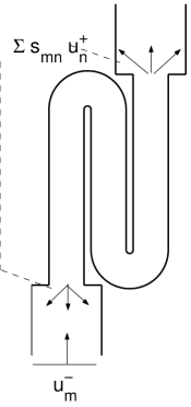
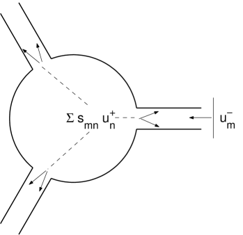
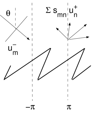
Figure 1: Various systems with nontrivial scattering properties: “quantum wire”, open resonator, diffraction grating. Dialing with the grating, one can reduce the problem to the strip whose width is equal to the grating’s period ($2\pi$ in the figure) with the quasi-periodical boundary conditions (2). All these systems can support trapped modes or guided waves.

In what follows let us restrict ourselves either by the Helmholtz $\Delta\psi+k^{2}n^{2}(x)\psi=0$ or by the Schrödinger $-\Delta\psi+V(x)\psi=E\psi$ equation and assume that for $|x|\geqslant R_{0}$ $n(x)\equiv 1$ or $V(x)\equiv 0$, respectively. Then modes $u_{n}^{\pm}(x)$ are solutions to the homogeneous problem for $|x|\geqslant R_{0}$. For example, the waveguide modes are $u_{n}^{\pm}=\phi_{n}(x_{\bot})\,e^{\pm i\lambda_{n}z}/\sqrt{\lambda_{n}}$, $\lambda_{n}=\sqrt{k^{2}-\mu_{n}}$ (or with $E$ instead of $k^{2})$, where $x=(z,x_{\bot})$, $z,x_{\bot}$ are local coordinates respectively along (outward to infinity) and across each channel, $\{\mu_{n},~{}\phi_{n}(x_{\bot})\}$ are eigenpairs to the problem in channel’s cross-section $z=\mathrm{const}$; the gratings modes are $u_{n}^{\pm}=\exp\{\pm i\lambda_{n}z+(n+\alpha)y\}/\sqrt{4\pi\lambda_{n}}$, $\lambda_{n}=\sqrt{k^{2}-\left(n+\alpha\right)^{2}}$ ($x_{\bot}=y$ is one-dimensional here) satisfy the quasi-periodical boundary conditions

$$\left.u\right|_{y=\pi}=e^{2\pi i\alpha}\left.u\right|_{y=-\pi}\,,\quad\partial_{y}\left.u\right|_{y=\pi}=e^{2\pi i\alpha}\partial_{y}\left.u\right|_{y=-\pi}$$ (2)

(here grating’s period equals to $2\pi$ and $\alpha=-k\sin\theta$, $\theta$ is the angle of incidence, see Fig. 1). It is also assumed in (1) that each mode differ from zero only at “its” channel: by $u^{\pm}_{n}$ we actually denote

$$u^{\pm}_{n}\leadsto u^{\pm}_{n}(z,x_{\bot})\eta(z)\,,$$ (3)

where $\eta(z)$ is a smooth cut-off function which equals to one inside the channel and zero elsewhere.

Modes with numbers $n$ such that $\lambda_{n}>0$ propagate (oscillate) along the channel at which they are defined; we distinguish outgoing and incoming (respectively, $u_{n}^{+}$ and $u_{n}^{-}$ in our notations) modes by the sign of the energy flux density $\mathrm{Im}\left(\frac{\partial u}{\partial\nu}\overset{-}{u}\right)$, where $\nu$ is the outward normal to channel’s cross-sections. At the threshold frequencies $\lambda_{n}=0$, and the above definition of modes failed; following the paper [1] we define threshold (standing) modes by the following replacement: $e^{\pm i\lambda_{n}z}/\sqrt{\lambda_{n}}\leadsto\left(1\mp z\right)/\sqrt{2}$.

The sum in (1) is normally taken over all propagating modes (including standing ones). Let the total number of such modes is $2N$. Then the space of solutions with asymptotics (1) is $N$-dimensional (see [1] again) and, consequently, there exists $N$ linearly independent rows $\left(c_{1}^{-},\dots,c_{N}^{-},c_{1}^{+},\dots,c_{N}^{+}\right)$, which form two $N\times N$ matrices $\mathbb{C}^{\pm}:=\|c_{mn}^{\pm}\|$. Both $\mathbb{C}^{\pm}$ are invertible (otherwise nontrivial solution to homogeneous problem with an asymptotics containing only outgoing or only incoming modes can exist). The unitary matrix $\mathbb{S}:=\left(\mathbb{C}^{-}\right)^{-1}\mathbb{C}^{+}$ is called “scattering matrix”. The question of its numerical determination was discussed in a long series of publications (see, e.g., [2, 3] as a most general method). The approach suggested below can be, in particular, applied to that end as well (see Section 3). However, our goal is a little bit wider.

Let us agree that $\mathrm{Im}\lambda_{n}\leqslant 0$ and include into the sum (1) all modes corresponding to $|\mathrm{Im}\lambda_{n}|<\gamma$ for some positive $\gamma$. Note that under our choice of the sign of $\mathrm{Im}\lambda_{n}$ modes $u_{n}^{-}$ are decay whilst $u_{n}^{+}$ are grow as $|x|\to\infty$, $n>N$. Now the question of interest is: is there exist linear combination of solutions (1) containing only decaying exponents? Existence of such a combination would indicate the solution to the homogeneous problem either localized at compact domain (trapped modes or bound states to waveguides and resonators) or propagating along a grating groove and decaying away from the grating (guided or surface grating waves).

Suppose the new matrix $\mathbb{C}^{+}$ is at our disposal and write it down as

$$\mathbb{C}^{+}=\left(\begin{array}[]{cc}C_{(11)}&C_{(12)}\\ C_{(21)}&C_{(22)}\end{array}\right)\,,$$

where the block $C_{(11)}$ is of size $N\times N$ and corresponds to the coefficients are in front of propagating modes. By straightforward verification one concludes that the condition

$$\det C_{(22)}=0$$ (4)

is sufficient for the existence of the aforementioned decaying solution. Consider (4) as the equation for the wave frequency $k$ (or particle energy $E$ in quantum physics). Thus we arrive to the existence criterion for localized solutions.

It can be also shown that scattering matrix $\mathbb{S}$ is now the left-upper block of the product $\left(\mathbb{C}^{-}\right)^{-1}\mathbb{C}^{+}$. Thus matrices $\mathbb{C}^{\pm}$ contain information about both scattering and trapping properties of the system.

However, the numerical determination of the matrices $\mathbb{C}^{\pm}$ is not a trivial task since the asymptotics (1) contains exponents that grow and decay with different rates. The leading term dominates, and all coefficients cannot be found accurately. The key point of the approach suggested in the next Section is to avoid this difficulty. In the Section 4 we give a very brief review on previously known numerical approaches and provide new examples of trapped modes.

2 Description of the approach

The main computational idea is as follows.

Consider the truncation of an infinite domain by removing infinite parts of all channels, starting from some distance $R>R_{0}$ (i.e., truncating lines are $z_{j}=R$, $j$ is the channel’s number). Let $\widehat{\psi}$ be the solution to the auxiliary problem which inherits all conditions of the original problem (at an infinite domain) with the following artificial condition at $z_{j}=R$:

$$\mathcal{B}_{j}\left(\widehat{\psi}-\sum_{n}\left(\widehat{c}^{-}_{n}u_{n}^{-}+\widehat{c}^{+}_{n}u_{n}^{+}\right)\right)=0\quad\forall j\,,\quad\mathcal{B}_{j}:=\left.\frac{\partial}{\partial z_{j}}+i\zeta\right|_{z_{j}=R}\,,$$ (5)

where $\zeta>0$ and coefficients $\widehat{c}_{n}^{\pm}$ are arbitrary.

Conditions (5) came into scene as the differentiation of the asymptotics (1) (positive $\zeta$ is necessary to avoid possible coincidence of $k^{2}$ with the spectrum of the auxiliary problem). Let us now try to chose coefficients $\widehat{c}^{\pm}_{n}$ in such a way that $\widehat{\psi}$ approximately agrees with the right-hand part in (1) at $z_{j}=R$. Thus one can expect that for sufficiently large $R$ the numbers $\widehat{c}^{\pm}_{n}$ are good approximations to $c_{n}^{\pm}$.

By this motivation we arrive to the condition on unknowns $\widehat{c}^{\pm}_{n}$: choose these coefficients in such a way that

$$\sum\limits_{j}\int\limits_{z_{j}=R}\left|\widehat{\psi}-\sum_{n}\left(\widehat{c}^{-}_{n}u_{n}^{-}+\widehat{c}^{+}_{n}u_{n}^{+}\right)\right|^{2}dx_{\bot}\mapsto\min\,.$$ (6)

It can be shown that the left-hand part in (6) goes to zero as $R\to\infty$ with exponential rate and

$$\sum_{n}\left|\,\widehat{c}^{\pm}_{n}-c^{\pm}_{n}\right|^{2}\underset{R\to\infty}{=}\mathrm{O}\left(\,e^{-\widehat{\gamma}R}\right)\,.$$

The proof of the similar convergence for the entries of the scattering matrix $\mathbb{S}$, as well as the estimation of the constant $\widehat{\gamma}$, can be found in [4, 5].

From (6), one has the simple algorithm to obtain approximations $\widehat{c}^{\pm}_{n}$ to $c^{\pm}_{n}$ that are sought for. In fact, the functional (6) is quadratic with respect to $\widehat{c}^{\pm}_{n}$. The Hermitian matrix of its coefficients can be written as

$$\left(\begin{array}[]{cc}\widehat{A}^{-}&\widehat{B}\\ \widehat{B}^{*}&\widehat{A}^{+}\end{array}\right)\,,$$ (7)

where

$$\widehat{A}^{\pm}_{pq}=\sum\limits_{j}\int\limits_{z_{j}=R}\left.\overline{\left(\widehat{u}_{p}^{\pm}-u_{p}^{\pm}\right)}\left(\widehat{u}_{q}^{\pm}-u_{q}^{\pm}\right)\right|_{z_{j}=R}dx_{\bot}\,,$$

$$\widehat{B}_{pq}=\sum\limits_{j}\int\limits_{z_{j}=R}\left.\overline{\left(\widehat{u}_{p}^{-}-u_{p}^{-}\right)}\left(\widehat{u}_{q}^{+}-u_{q}^{+}\right)\right|_{z_{j}=R}dx_{\bot}\,,$$

and the functions $\widehat{u}_{n}^{\pm}$ are the solutions to the problems with artificial conditions $\mathcal{B}_{j}\left(\widehat{u}_{n}^{\pm}-u_{n}^{\pm}\right)=0$.

Note that the data to the auxiliary problems on the differences $\left(\widehat{u}_{n}^{\pm}-u^{\pm}_{n}\right)$ don’t contain growing as $R\to\infty$ exponents as well as summation of different rate exponents. These problems have to be solved numerically by means of any appropriate method (e.g., finite element method).

Finally, given the matrix (7) one can find its spectrum and select $M$ smallest magnitude eigenvalues and corresponding eigenvectors $h_{1},\dots,h_{M}$ (here $2M$ denotes the size of the matrix) and put

$$\left(\begin{array}[]{c}\widehat{\mathbb{C}}^{-}\\ \widehat{\mathbb{C}}^{+}\end{array}\right)=\left(h_{1},\dots,h_{M}\right)\,.$$ (8)

This finalize the description of the computation procedure. It is clear that the approach doesn’t sensitive to the geometry of a problem.

3 Examples of scattering data computation

In this section we discuss the the application of the above approach to the computation of scattering data.

1 Quantum control on electron stream

Consider the two-dimensional domain $D\subset\mathbb{R}^{2}$ consisting of a resonator (i.e., of a disk of radius $\rho_{0}$) which is connected to infinity by means of three straight channels (waveguides) of width $d$ (see the left part in Fig.2); directions of axes of two channels (say, 2nd and 3rd) are symmetric with respect to the direction of the 1st channel axis (the symmetry is not essential and is introduced to decrease the number of problem parameters). We assume that the motion of an electron is bounded by the domain $D$ and the wave function $\psi(x,y)$ vanishes at the boundary of $D$.

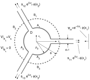
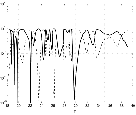
Figure 2: Left: Sketch of the model. Right: Transporting losses $|s_{11}|^{2}+|s_{13}|^{2}$ (solid line) and the transmission coefficient $|s_{12}|^{2}$ (dashed line) versus energy $E$ of an incident electron; handling potentials are fixed as $V_{1}=0$, $V_{2}=V_{3}=(1.5\pi)^{2}\sim 22.2$; the size of resonator $\rho_{0}=3d$.

The governing potential $V$ is induced in the following way. Let the resonator’s walls $A_{1}$, $A_{2}$, $A_{3}$ are charged by potentials $V_{1}$, $V_{2}$, $V_{3}$, respectively; the handling is realized by variation of values $V_{1,2,3}$. The whole system is shielded by three non-closed lines $B_{1}$, $B_{2}$, $B_{3}$, each shield $B_{j}$ consists of a segment of radius $B$ and two rays directed along channel’s walls (these shields are shown in Fig.2 by dashed lines). Thus the potential $V$ is the solution to Laplace equation in the unbounded domain $D_{B}$ (restricted by the shields $B_{1,2,3}$) and satisfies the Dirichlet boundary conditions $\left.V\right|_{A_{j}}=V_{j}$, $\left.V\right|_{B_{j}}=0$. It is known that such solution exponentially decays along the channels. It allows to accept, as an approximation to $V$, the solution to the problem in a finite part of $D_{B}$ that is located inside the disk of sufficiently large radius $B$ (with the zero boundary condition at new boundaries).

We consider the scattering problem in the domain $D$ under the energy range $\pi^{2}<E<(2\pi)^{2}$ (in reduced units), that is, between first and second thresholds and, consequently, the size of the scattering matrix is $3\times 3$ (one propagating mode at each channel). The examined energy range corresponds to realistic energy values $(0.01\div 1)\,$ev for $d=(1\div 10)\,$nm.

Let the incident electron stream comes along the 1st channel, so the scattering data is collected in the first row $\|s_{1j}\|$, $j=1,2,3$, of the scattering matrix $\mathbb{S}$. Now the question is if one can choose any combination of the energy $E$ and handling potentials $V_{1}$, $V_{2}$, $V_{3}$ such that the transport of an electron stream either to 2nd or to 3rd channel is close to certain (i.e., either $\left|s_{12}\right|^{2}\approx 1$ or $\left|s_{13}\right|^{2}\approx 1$)? If yes, the transport can be switch from second to third channel by trading places of $V_{1}$ and $V_{3}$.

Some of the results are given in the right-part in Fig.2. It is seen that transporting losses can be reduced below 0.1% by variation of $E$ (the same effect can be achieved by variation of $V$ as well, not shown here).

2 Conductance of bent waveguides

Two-dimensional bent waveguides are often considered as models of microwave devices or quantum wires (see [8]). Scattering problem for such a model is to determine the matrix $\mathbb{S}$ corresponding to the solution of the free Schrödinger (Helmholtz) equation in a curved strip with asymptotics (1) and satisfying Dirichlet boundary conditions. Normally the implementation of a device presumes the strip of piecewise constant width (e.g., a bent waveguide is connected to open leads, as shown in the left part of Fig.3); this case the definition of modes and scattering matrix is related to leads.

Typically the wave process in a system is energized by an incoming single mode (number $m$) of inlet lead, and the observed quantity is the normalized conductance $G_{m}=\sum_{n}\left|s_{mn}\right|^{2}$, where sum is taken over all outgoing modes of outlet lead.

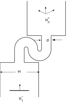
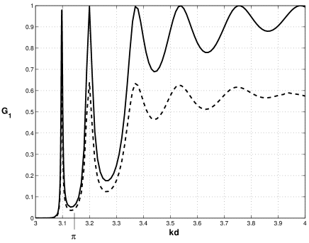
Figure 3: Left: A bent waveguide (numerous dimensions of the bend are not specified) of width $d$ connected with two open leads of width $H$; Right: Normalized conductance $G_{1}$ (due to the lowest mode in the lead) versus dimensionless frequency $kd$: solid line — $H/d=2$, dashed line — $H/d=4$. Note that the location of conductance maxima doesn’t depend on the ratio $H/d$ and the first peak is observed (below the bent waveguide threshold $\pi$) at $kd\approx 3.097$ (compare with the trapped mode frequency for the waveguide with the same bent part, see Fig.5).

It is clear that modes can propagate throughout the leads at frequencies below the threshold ($kd=\pi$) of the bent strip. Transmission of energy at such frequencies through the bend is classically forbidden. However, that becomes possible due to quantum effects. The computation results are shown in the right part of Fig.3: the first conductance peak is observed below the threshold; above the threshold, the conductance exhibits an oscillating behavior. The frequency corresponding to the first conductance peak is close to the trapped frequency of the infinite bent waveguide (see Section 4) and can be thought as resonance frequency.

4 Computation of trapped modes: brief review and new examples

The localized solutions have been attracted a lot of attention during last decades as examples of nonuniqueness to a scattering problem which, at the same time, exhibit abnormal physical properties. Depending on the area of application these solutions are either called trapped modes (microwave and/or acoustic waveguides, water waves), or bound states (quantum wires and photonic crystals), or guided (Rayleigh-Bloch) waves (diffraction gratings). The framework of a workshop publication doesn’t suit for detailed review of tens of papers devoted to the subject. The whole spectrum of papers can be conventionally divided into three categories: proof of existence or non-existence of trapped modes, asymptotic estimate of trapped eigenfrequencies (energies) and numerical approaches. Not mention the first category completely, we point out the key names and selected papers related to the last two categories. The more comprehensive review in a part related to the quantum applications can be found in the book [7].

Concerning waveguide problems, the asymptotic results can normally be obtained if the geometry is a perturbation of a straight strip. This may be a case for small indentation [8], laterally coupled waveguides through small window(s) [9], slightly curved strips and tubes [10], etc. (see, e.g., [11] for asymptotic results in gratings). Normally, the asymptotic formulas match numerical computation for some range of “small” parameter; at the same time, numerics is often fails when perturbation becomes very small.

As far as known to the author, the overwhelming majority of papers dedicated to the numerical detection of trapped modes dealt with objects of a relatively simple geometry. The typical methods were either the separation of variables in sub-domains with subsequent matching of infinite series, or the reduction of a problem to the integral equation (the explicit knowledge of Green’s function is required), or the application of a variational technique (the sufficiently reach set of trial functions satisfying boundary conditions is required). All these methods were successfully utilized and a wide variety of trapped modes found by research groups represented by papers [7, 10, 12, 13].

However, all the mentioned methods are of limited universality and applicability range. The developed approach allows us to contribute into the scope providing successfully found new examples of trapped modes. Due to the generality of the approach the list of examples can be very wide, below are few of them.

The Dirichlet trapped modes eigenfrequencies for the straight waveguide with a local indentation are shown in Fig.4. Such model was the subject of rigorous studies in [8] where existence of trapped modes below the threshold were proved and asymptotic estimate of them found. In Fig.4 the numerical results are given in comparison with the asymptotic formulas of [8]. It is seen that both results match each other although the range of applicability of asymptotic formulas is relatively narrow.

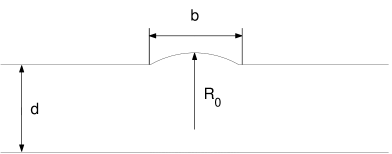
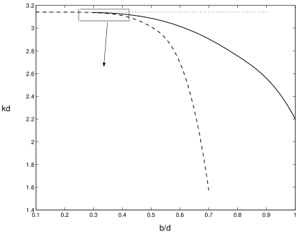
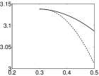
Figure 4: Left: Waveguide with an one-side indentation. Right: The Dirichlet mode trapped eigenfrequencies $kd$ (solid line) versus the length $b/d$ of the indentation (whilst $R_{0}/d=1$) in comparison with the asymptotic results of the paper [8] (dashed line); the inset shows the vicinity of the threshold in an expanded range.

Examples in Fig.5 concern the trapped modes for that no numerical estimates were known. In the left part we show the map of $|\psi_{trapped}(x,y)|$ for a bent waveguide which bent structure is the same as in the example of Fig.3 (but with no leads attached). After replacing of the waveguide’s straight parts by wider leads the eigenfrequency (energy) of this trapped mode moves to a resonance in the complex plane. This resonance works as a “bridge” providing the sub-threshold conductance peak in Fig.3.

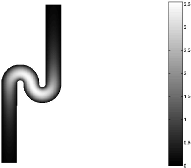
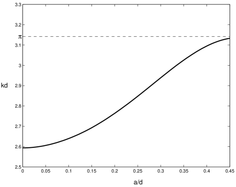
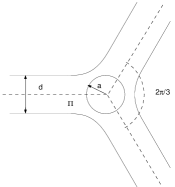
Figure 5: Left: The intensity map of the trapped mode in a bent waveguide; the bent part is the same as in Fig.3, trapped mode frequency is $kd\approx 3.091$ (which is slightly below the sub-threshold conductance frequency for the bent waveguide with adjoint leads, see Section 2). Right: The dimensionless trapped eigenfrequencies $kd$ (versus the size of disk hole) for the domain shown in the inset.

In the right part of Fig.5 we provide an example of trapping properties of the domain with relatively complicated geometry. The domain in question consists of three smoothly and symmetrically connected channels (the symmetry and the number of channels are not essential); some disk is taken out around the symmetry center. The Dirichlet boundary conditions are assumed at the outdoor domain boundaries whilst the Neumann conditions are set at the interior circle boundary. This domain with no hole ($a/d=0$) can be thought as a bent waveguide with an “infinite” indentation, thus the existence of the Dirichlet trapped mode below the threshold can be clearly predicted, and it is numerically found as $kd\approx 2.594$. The trapped eigenfrequencies approaches the threshold versus increasing the disk hole radius.

5 Conclusion

The general approach for numerical computation of scattering and trapping properties of systems with finitely many channels to infinity quantum, microwave and optics physics was discussed. The approach can be adopted for the numerical search of resonances for the same type of scattering systems; this work is under development.

References

- [1] S. A. Nazarov, B. A. Plamenevskii. Elliptic problems in domains with piecewise smooth boundaries. Walter de Gruyter, Berlin, 1994.
- [2] Ch.I.Goldstein. A finite element method for solving Helmholtz type equations in waveguids and other unbounded domains. Mathematics of Computation, 39 (1982), 309–324.
- [3] J.Elschner, G.Schmidt. Numerical solution of optimal design problems for binary gratings. Journal of Computational Physics, 146 (1998), 603-626.
- [4] V.E.Grikurov, E.Heikkola, P.Neittaanmäki, B.A.Plamenevskii. On computation of scattering matrices and on surface waves for diffraction gratings. Numerische Mathematik, 94 (2003), no.2, pp.269–288.
- [5] V.O.Kalvine, P.Neittaanmäki, B.A.Plamenevskii. On scattering matrices for self-adjoint elliptic problems in domains with cylindrical ends. Reports of the Department of Mathematical Information Technology. Series B. Scientific Computing, No. B 18/2002, University of Jyväskylä, 2002; On a method of search for trapped modes in domains with cylindrical ends. “WAVES 2003” Proceed. of the Sixth Int. Conf. on Math. and Numer. Aspects of Wave Propagation, Springer, 2003, pp.469-474.
- [6] L.M.Baskin, V.E.Grikurov, P.Neittaanmaki, B.A.Plamenevskii. On quantum phenomena in control of electron flows. Letters Journ. Technical Phys. vol.30 (2004), no.15, pp.62-69 (to appear).
- [7] J.T.Londergan, J.P.Carini, D.P.Murdock. Binding and scattering in two-dimensional systems. Application to quantum wires, waveguides and photonic crystals. Springer-Verlag, Berlin, 1999.
- [8] W.Bulla, F.Gesztesy, W.Renger, B.Simon. Weakly coupled bound states in quantum waveguides. Proceedings of the American Mathematical Society, 125 (1997), 1487-1495.
- [9] I.Yu.Popov. Asymptotics of bound states for laterally coupled waveguides. Reports on mathematical physiscs, 43 (1999), 427; S.V.Frolov, I.Yu.Popov. Resonances for laterally coupled quantum waveguides. Journal Of Mathematical Physics, 41 (2000), 4391–4405.
- [10] P.Exner, P.Seba, M.Tater, D.Vanek. Bound states and scattering in quantum waveguides coupled laterally through a boundary window. J. Math. Phys., 37 (1996), 4867-4887; P.Duclos, P.Exner, D.Krejcirik. Bound states in curved quantum layers. Commun. Math. Phys., 223 (2001), 13-28; E.N.Bulgakov, P.Exner, K.N.Pichugin, A.F.Sadreev. Multiple bound states in scissor-shaped waveguides. Phys. Rev. B, 66 (2002), 155109; D.Borisov, P.Exner. Exponential splitting of bound states in a waveguide with a pair of distant windows. J. Phys. A, 37 (2004), 3411-3428.
- [11] I.V.Kamotsky, S.A.Nazarov. Wood anomalies and surface waves in problems of scattering by a periodic boundary. Mat. Sb., 190, (1999) 43–70, 109-138.
- [12] R.Porter, D.V.Evans. Rayleigh-Bloch surface waves along periodic gratings and their connection with trapped modes in waveguides. J. Fluid Mech., 386 (1999) 233–258; R.Porter, D.V.Evans. On existence of embedded surface waves along arrays of parallel plates. Quartly Journal on Mechanics and Applied Mathematics, 55 (2002), 481–494.
- [13] P.McIver, C.M.Linton, M.McIver. Construction of trapped modes for wave guides and diffraction gratings R. Soc. Lond. Proc. Ser. A Math. Phys. Eng. Sci., 454, (1998) 2593–2616; Y.Duan, M.McIver. Rotational acoustic resonances in cylindrical waveguides. Wave Motion, 39 (2004), 261-274.