Negativity of the Wigner function as an indicator of nonclassicality

Abstract

A measure of nonclassicality of quantum states based on the volume of the negative part of the Wigner function is proposed. We analyze this quantity for Fock states, squeezed displaced Fock states and cat-like states defined as coherent superposition of two Gaussian wave packets.

e-mail: kenfack@mpipks-dresden.mpg.de    karol@cft.edu.pl

I Introduction

Analyzing pure quantum states in an infinite dimensional Hilbert space it is useful to distinguish a family of coherent states, localized in the classical phase space and minimizing the uncertainty principle. These quantum analogues of points in the classical phase space are often considered as ’classical’ states. For an arbitrary quantum state one may pose a natural question, to what extent it is ’nonclassical’ in a sense that its properties differ from that of coherent states. In other words, is there any parameter that may legitimately reflect the degree of nonclassicality of a given quantum state? This question was motivated with the first observation of nonclassical features of electromagnetic fields such as sub-poissonian statistics, antibunching and squeezing. Additionally, it is well known that the interaction of (non)linear devices with quantum states may flip from one state to another; for instance, nonlinear devices may produce nonclassical states from their interaction with the vacuum or a classical field. A systematic survey of nonclassical properties of quantum states would be worthwhile because of the nowadays ever increasing number of experiments in nonlinear optics. An earlier attempt to sheding some light on the nonclassicality of a quantum state was pioneered by Mandel Ma79 , who investigated the radiation fields and introduced a parameter ${\bf q}$ measuring the deviation of the photon number statistics from the Poissonian distribution, characteristic of coherent states.

In general, to define a measure of nonclassicality of quantum states one can follow several different approaches Do02 . Distinguishing a certain set $\cal C$ of states (e.g. the set of coherent states $|\alpha\rangle$), one looks for the distance of an analyzed pure state $|\psi\rangle$ to this set, by minimizing a distance $d(|\psi\rangle,|\alpha\rangle)$ over the entire set $\cal C$. Such a scheme based on the trace distance was first used by Hillery Hi87 ; Hi89 , while other distances (Hilbert-Schmidt distance DMMW00 ; DR03 or Bures distance MMS02 ; MMS03 ) were later used for this purpose. The same approach is also applicable to characterize mixed quantum states: minimizing the distance of the density $\rho$ to the set of coherent states is related DR03 ; ABM03 to the search for the maximal fidelity (the Hilbert-Schmidt fidelity ${\rm Tr}\left(\rho\sigma\right)$ or the Bures-Uhlmann fidelity $\left({\rm Tr}\sqrt{\rho^{1/2}\sigma\rho^{1/2}}\right)^{2}$) with respect to any coherent state, $\sigma=|\alpha\rangle\langle\alpha|$. On the same footing, the Monge distance introduced in zs98 ; zs01 may be applied to describe, to what extent a given mixed state is close to the manifold of coherent states.

Yet another way of proceeding is based on the generalized (Cahill) phase space representation $R_{\tau}$ of a pure state, which interpolates between the Husimi ($Q$), the Wigner ($W$) and the Glauber–Sudarshan ($P$) representations. The Cahill parameter $\tau$ is proportional to the variance of a Gaussian function one needs to convolute with $P$ representation to obtain $R_{\tau}$ CG69 . In particular for $\tau=1,1/2,0$ one obtains the Q-, W- and P- representations, respectively. By construction the $Q$ representation is non-negative for all states, while the Wigner function may admit also negative values, and the $P$ representation may be singular or may not exist.

The smoothing effect of $R_{\tau}$ is enhanced as $\tau$ increases. If $\tau$ is large enough so that $R_{\tau}$ becomes positive definite regular function, thus acceptable as a classical distribution function, then the smoothing is said to be complete. The greatest lower bound $\tau_{m}$ for the critical value was adopted by Lee Le91 ; Le92 , as nonclassical depth of a quantum state and this approach was further developed in LB95 ; MBGB01 ; MB03 . The limiting value, $\tau_{m}=1$, corresponds to the $Q$ function which is always acceptable as a classical distribution function. The lowest value, $\tau_{m}=0$, is ascribed to an arbitrary coherent state because its $P$ function is a Dirac delta function, so its $\epsilon$–smoothing becomes regular. The range of $\tau_{m}$ is thus $\tau_{m}\in[0,1]$.

If the Husimi function of a pure state admits at least one zero $Q(\alpha_{0})=0$, then a Cahill $R_{\tau}$ distribution with a narrower smearing, $\tau<1$, becomes negative in the vicinity of $\alpha_{0}$. Therefore the classical depth for such quantum states is maximal, $\tau_{m}=1$ LB95 . The only class of states, for which $Q$ representation has no zeros, are the squeezed vacuum states, for which $\tau_{m}$ is a function of the squeezing parameter $s$. In the limiting case $s=0$ one obtains the coherent state for which the $R_{0}=P$ distribution is a Dirac delta function, that is $\tau_{m}=0$.

A closely related approach to characterizing quantum states is based on properties of their Wigner functions in phase space $\{p,q\}$. One can prove that the Wigner function is bounded from below and from above CG69 . In the normalization $\iint W(q,p)dqdp=1$ used later in this work, such a bound reads $|W(q,p)|\leq 1/\pi\hbar$. Further bound on integrals of the Wigner function were derived in BDW99 , while an entropy approach to the Wigner function was developed in MF00 ; Wl01 .

In order to interpret the Wigner function as a classical probability distribution one needs to require that $W$ is non–negative. As found by Hudson in 1974 Hu74 , this is the case for coherent or squeezed vacuum states only. A possible measure of nonclassicality may thus be based on the negativity of the Wigner function which may be interpreted as a signature of quantum interference.

The negativity of the Wigner function has been linked to nonlocality, according to the Bell inequality bell87 , while investigating the original Einstein-Podolsky-Rosen (EPR) state einst35 . In fact Bell argued that the EPR state will not exhibit nonlocal effects because its Wigner function is everywhere positive, and as such will allow for a hidden variable description of correlations. However, it is now demonstrated banas98 ; cohen97 that the Wigner function of the EPR state, though positive definite, provides a direct evidence of nonlocality. This violation of the Bell’s inequality holds true for the regularized EPR state banas99a and also for a correlated two-mode quantum state of light banas99b .

It is also worth recalling that the Wigner function can be measured experimentally SXX93 , including the measurements of its negative values NRO00 . The interest put on such experiments has triggered a search for operational definitions of the Wigner functions, based on experimental setup Le97 ; Lou03 .

The aim of this letter is to study a simple indicator of the nonclassicality, which depends on the volume of the negative part of the Wigner function. To demonstrate a potential use of such an approach we investigate certain families of quantum states. The nonclassicality indicator is defined in section 2. The Schrödinger cat state, being constructed as coherent superposition of two Gaussian wave packets, is analyzed in section 3 while section 4 is devoted to Fock states and to the squeezed displaced Fock states. Finally in section 5, a brief discussion of results and perspectives is given.

II The nonclassicality indicator

The Wigner function of a state $|\psi\rangle$ defined by Wi32 ; HCSW84

$$W_{\psi}(q,p)=\frac{1}{2\pi}\int_{-\infty}^{+\infty}dx\langle q-\frac{x}{2}|\psi\rangle\langle\psi|q+\frac{x}{2}\rangle\exp\left(ipx\right)$$ (1)

satisfies the normalization condition $\iint W_{\psi}(q,p)dqdp=1$. Hence the doubled volume of the integrated negative part of the Wigner function may be written as

$$\delta(\psi)=\iint\left[|W_{\psi}(q,p)|-W_{\psi}(q,p)\right]dqdp=\iint|W_{\psi}(q,p)|dqdp-1\ .$$ (2)

By definition, the quantity $\delta$ is equal to zero for coherent and squeezed vacuum states, for which $W$ is non-negative. Hence in this work we shall treat $\delta$ as a parameter characterizing the properties of the state under consideration. Similar quantities related to the volume of the negative part of the Wigner function were used in Sc99 ; BBCDFS02 ; DMWS04 to describe the interference effects which determine the departure from classical behaviour.

Furthermore, a closely related approach was recently advocated by Benedict and collaborators BC99 ; FCM02 . Their measure of the nonclassicality of a state $|\psi\rangle$ reads

$$\nu(\psi)=1-\frac{I_{+}(\psi)-I_{-}(\psi)}{I_{+}(\psi)+I_{-}(\psi)}$$ (3)

where $I_{+}(\psi)$ and $I_{-}(\psi)$ are the moduli of the integrals over those domains of the phase space where the Wigner function is positive and negative, respectively. The normalization condition implies $I_{+}-I_{-}=1$, so that $\nu=2I_{-}/(2I_{-}+1)$ leads to $0\leq\nu<1$. Using this notation we may rewrite (2) as $\delta=I_{+}+I_{-}-1=2I_{-}$ and obtain a simple relation between both quantities

$$\nu=\frac{2I_{-}}{1+2I_{-}}=\frac{\delta}{1+\delta}$$ (4)

with $\delta=\nu/(1-\nu)$. It turns out that both quantities are equivalent in the sense that they induce the same order in the space of pure states: the relation $\delta(\psi_{1})>\delta(\psi_{2})$ implies $\nu(\psi_{1})>\nu(\psi_{2})$. However, from a pragmatic point of view there exists an important difference between both quantities.

To compute explicitly the quantity (3) one faces a difficult task to identify appropriately the domains, in which the integration has to be carried out. On the other hand, knowing the Wigner function $W(q,p)$ of a quantum state, it is straightforward to get its absolute value and to evaluate numerically the integration (2).

Let us emphasize again that the Hilbert space containing all pure states is huge, so one should not expect to characterize the nonclassical features of a quantum state just by a single scalar quantity. Our approach focuses on a particular issue, whether the Wigner function is positive and may be interpreted as a classical probability distribution. Therefore, the proposed indicator $\delta$ should be considered as a tool complementary to these worked out earlier and reviewed above.

III The Schrödinger cat

A quantum state, called Schrödinger cat, is a coherent superposition of two coherent states localized in two distant points of the configuration space, $\pm q_{0}$. The wave function of such a state reads in the position representation

$$\Psi(q)=\frac{N}{\sqrt{2}}\left[\phi_{+}(q)+\phi_{-}(q)\right]$$ (5)

where

$$\phi_{\pm}(q)=\left(\frac{m\omega}{\pi\hbar}\right)^{1/4}\exp\left(-\frac{m\omega}{2\hbar}(q\pm q_{0})^{2}+i\frac{p_{0}}{\hbar}(q\pm q_{0})\right)\ .$$ (6)

From now on atomic units are used $(m=\hbar=\omega=1)$. In other words we measure the size of the product $pq$ in units of $\hbar$. The classical limit $\hbar\rightarrow 0$ means the action $pq$ characteristic of the system is many order of magnitude larger than $\hbar$. A glance on Eq. (6) reveals that the phase, governed by $p_{0}$, is of great importance in that it induces oscillations on the wave function as can be seen in Fig.1. Note that the normalization constant $N$ depends on the location of the centers $(q_{0},p_{0})$ of both coherent states that make up the cat state. Therefore one sees that the Wigner function may depend not only on the distance $2q_{0}$ between the both states, but also on their momentum, $p_{0}$. So far, the studies on the cat states Le97 were usually restricted to the case of standing cats, $p_{0}=0$. In this letter we demonstrate that the parameter $p_{0}$ influences the shape of the Wigner function, in particular, if $q_{0}\sim 1$ and both packets are not spatially separated.

Inserting $(\ref{wftion})$ into the Wigner function (1) one obtains

$$W_{\Psi}(q,p)=W_{+}(q,p)+W_{-}(q,p)+W_{int}(q,p)\ .$$ (7)

Here

$$W_{\pm}(q,p)=\frac{N^{2}}{2\pi}\exp\left(-(q\pm q_{0})^{2}-(p-p_{0})^{2}\right)$$ (8)

represent two peaks of the distribution centered at the classical phase space points $(\pm q_{0},p_{0})$, while

$$W_{int}(q,p)=\frac{N^{2}}{\pi}\cos\left(2pq_{0}\right)\exp\left(-q^{2}-(p-p_{0})^{2}\right)$$ (9)

stands for the interference structure which appear between both peaks. Normalizing (5) yields

$$N=\left(1+\cos\left(2p_{0}q_{0}\right)\exp\left(-q_{0}^{2}\right)\right)^{-1/2}\ .$$ (10)

Making use of the formula (7) for the Wigner function of the cat state $|\Psi\rangle$ its nonclassicality parameter

$$\delta(\Psi)=\iint\left|W_{+}(q,p)+W_{int}(q,p)+W_{-}(q,p)\right|dqdp-1$$ (11)

may be approximated by

$$\delta(\Psi)\approx N^{2}\left[1+\int\frac{dp}{\sqrt{\pi}}\left|\cos\left(2pq_{0}\right)\right|\exp\left(-(p-p_{0})^{2}\right)\right]-1\ .$$ (12)

Strictly speaking the right hand side of equation (12) forms an upper bound for $\delta(\Psi)$, which may be practically used as its fair approximation. Because of the oscillations of the absolute value of cosine, it is difficult to perform the integration analytically. In the special case $q_{0}=0$, the superposition of coherent states (5) reduces to a single coherent state and correspondingly (12) leads to $\delta(\Psi)=0$.

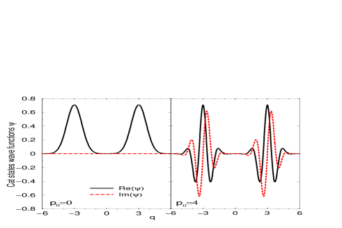
Figure 1: Schrödinger cat states wave functions plotted with $p_{0}=0$ (left) and with $p_{0}=4$ (right). Dashed and solid lines represent the imaginary and the real part of the wave function, respectively. Notice that the envelopes of both wave functions do coincide.

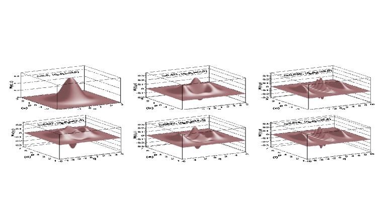
Figure 2: Plots of the Wigner functions of the Schrödinger cat states (7). Each panel is labeled by the separation distance $q_{0}$, the momentum $p_{0}$ and the resulting indicator $\delta$. Observe that for intermediate separations, $q_{0}\sim 1$, the indicator $\delta$ changes with $p_{0}$. Upper row shows the ’standing cats’ ($p_{0}=0$) while the cats in motion ($p_{0}=4$) are represented in the lower row

Fig. 2 shows plots of the Wigner function of the cat states for several values of the separation $q_{0}$ and the momentum $p_{0}$. One clearly sees the formation of the quantum interference structure halfway between the two humps as the separation distance $q_{0}$ increases. The frequency of the interference structure increases with the separation Le97 . For intermediate separations ($0<q_{0}\leq 4$), the Wigner function changes its structure with $p_{0}$, see fig.2b and 2c. However, for a larger separation distance, $q_{0}>4$, the Wigner function for $p_{0}=p_{1}\neq 0$ may be approximated by the Wigner function for the state with $p_{0}=0$ translated by a constant vector $\Delta p=p_{1}$.

In the case of ’standing cats’, ($p_{0}=0$), the indicator $\delta$ increases monotonically with the separation $q_{0}$, and reflects presence of the interference patterns at $q=0$ - see Fig. 4k. The growth of the nonclassicality saturates at $q_{0}\approx 4$, as the interference patterns become practically separated from both peaks, and the parameter $\delta$ tends to the limiting value, $\delta_{max}\approx 0.636$. In the limit $q_{0}\rightarrow\infty$ the oscillations of the cosine term in Eq. (12) become rapid and a crude approximation $|\cos(q_{0}p_{0})|\approx 1$ gives an explicit upper bound $\delta\leq 2N^{2}-1\approx 1$.

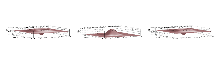
Figure 3: As in Fig. 2. The values of $q_{0}$ labeling each panel, correspond to the successive extrema (g,h,i) of the indicator $\delta$ plotted in Fig. 4m as a function of $q_{0}$. Wigner funtion for the ’Cats in motion’ as in lower row of Fig.2, for the selected values of $p_{0}$, for which the dependence $\delta(q_{0})$ achieves its extrema.

This picture gets more complicated for the states with $p_{o}\neq 0$, in particular for a small separation distance, $(0<q_{0}\leq 4)$. In this case, $\delta$ exhibits oscillations as shown in Fig.4l, 4m, 4n. To shed some light on this behavior we have chosen to plot in Fig.3 the Wigner function for which $\delta(q_{0})$ achieves extremal values. For instance, $\delta$ at $q_{0}=0.725$ (Fig. 3b) is smaller than at $q_{0}=0.4$ (Fig. 3a) or $1.175$ (Fig. 3c). This is due to the the interference structure, which is not symmetric with respect to the reflection $p\to-p$, in contrast to the case of cats with $p_{0}=0$.

As shown in Fig. 4, the frequency of oscillations increases with $p_{0}$, but the limiting value $\delta(q_{0}\to\infty)$ does not depend on the initial momentum $p_{0}$. This can also be demonstrated, investigating the dependence of the quantity $\delta$ as a function of $p_{0}$. As follows from Eq. (12), the indicator $\delta$ displays regular oscillations with the period $p_{osc}=\pi/q_{0}$ – See Fig. 5. In other words a non–zero separation parameter $q_{0}$ breaks the translational invariance in momentum and introduces a characteristic momentum scale $p_{osc}\sim 1/q_{0}$. Note that the amplitudes of the oscillations decrease fast with $q_{0}$, so that for well separated cats with $q_{0}>4$ the quantity $\delta$ is practically independent on $p_{0}$.

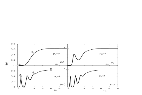
Figure 4: Indicator $\delta$ of the Schrödinger cat state $|\psi\rangle$ as a function of the separation distance $q_{0}$ and several values of $p_{0}$ as labelled on each panel. Grey dots (a-f) refer to labels of individual panels of Fig. 2. while grey dots (g,h,i) refer to that of fig.3.

Figure 5: Indicator $\delta$ of the Schrödinger cat state $|\Psi\rangle$ as a function of the momentum $p_{0}$ for certain values of the separation $q_{0}$.

IV Generalized Fock states

Let us consider the squeezed displaced Fock state defined by

$$|\beta,\eta,n\rangle=S(\eta)D(\beta)|n\rangle\ ,$$ (13)

where $|n\rangle$ is the original Fock state and $n=0,1,2,\dots$. The displacement $D(\beta)$ and the squeezed $S(\eta)$ operators are defined by MW95 ; Le97

$$D(\beta):=\exp(\beta a^{\dagger}-\beta^{*}a){\rm\quad and\quad}S(\eta):=\exp\left(\frac{1}{2}(\eta^{*}a^{2}-\eta a^{\dagger 2})\right),$$ (14)

where $a$ and $a^{\dagger}$ are usual photon annihilation and creation operators, respectively. The complex variable $\beta$ represents the magnitude and angle of the displacement. Similarly, writing the complex number in its polar form, $\eta=s\exp(i\phi)$, it is easy to see that the radius $s$ plays the role of the squeezing strength while the angle $\phi$ indicates the direction of squeezing. It was shown in CG69 that the displacement operators $D(\beta)$ form a complete set of operators. Thus any bounded operator $F$, (for which the Hilbert-Schmidt norm $\parallel F\parallel=\sqrt{{\rm Tr}(F^{\dagger}F)}$ is finite), can be expressed in the form $F=\int f(\xi)D^{-1}(\xi){d^{2}\xi}/{\pi}$ in which the weight function $f(\xi)={\rm Tr}(FD(\xi))$ is unique and square-integrable. Given that every density operator is bounded (${\rm Tr}(\rho^{\dagger}\rho)={\rm Tr}(\rho^{2})\leq 1$), one may write an arbitrary density operator $\rho=\int\chi(\xi)D^{-1}(\xi){d^{2}\xi}/{\pi}$. Here the weight function $\chi(\xi)={\rm Tr}(\rho D(\xi))$ is just the expectation value of the displacement operator commonly known as characteristic function. The complex Fourier transform of $\chi(\xi)$ defines the Wigner function

$$W(\alpha)=\int\frac{d^{2}\xi}{\pi}\chi(\xi)\exp(\xi^{*}\alpha-\xi\alpha^{*})\ .$$ (15)

One may therefore express $\chi(\xi)$ in terms of the Wigner function by performing the inverse Fourier transform as

$$\chi(\xi)=\int\frac{d^{2}\alpha}{\pi}W(\alpha)\exp(\xi\alpha^{*}-\xi^{*}\alpha)\ ,$$ (16)

so that upon substitution into the density operator expression above, one gets

$$\rho=\int\frac{d^{2}\alpha}{\pi}W(\alpha)T(\alpha)\ .$$ (17)

The operators $T(\alpha)$ denote

$$T(\alpha) = \int\frac{d^{2}\xi}{\pi}\exp(\xi\alpha^{*}-\xi^{*}\alpha)D^{-1}(\xi)$$ (18)

$$= 2D(\alpha)(-1)^{a^{\dagger}a}D^{-1}(\alpha)\ ,$$

so that the Wigner function may be interpreted as a weight function for the expansion of the density operator in terms of the operators $T(\alpha)$ CG69 . These operators are Hermitian, $T=T^{\dagger}$, and possess the same completeness properties as the displacement operators $D(\alpha)$. Making use of the parity operator $(-1)^{a^{\dagger}a}=\exp(i\pi a^{\dagger}a)$, one finally shows that

$$W(\alpha)=2(-1)^{n}{\rm Tr}(\rho D(2\alpha))$$ (19)

with $n=a^{\dagger}a$ being the photon number.

In the case of the squeezed displaced Fock states, $\rho=|\beta,\eta,n\rangle\langle\beta,\eta,n|$, the Wigner function becomes

$$W_{n}(\alpha)=2(-1)^{n}\langle\beta,\eta,n|D(2\alpha)|\beta,\eta,n\rangle$$ (20)

Performing explicitly calculations of matrix elements, one obtains :

$$W_{n}(\alpha)=\frac{2}{\pi}(-1)^{n}\exp(-2|b|^{2})L_{n}(4|b|^{2})$$ (21)

with $b=\cosh(s)(\alpha^{*}-\beta^{*})+\exp(-i\phi)\sinh(s)(\alpha-\beta)$kader03 . Here $L_{n}$ denotes the Laguerre polynomial of the $n$-th order.

Figure 6: The nonclassicality indicator $\delta(|n\rangle)$ of the Fock states versus the quantum number $n\leq 250$ (solid line). Dashed line represents $\frac{1}{2}\sqrt{n}$ plotted for comparison.

The Wigner function (21) allows us to compute the nonclassicality parameter $\delta(|\beta,\eta,n\rangle)$ for a given displaced squeezed Fock state $|\beta,\eta,n\rangle$. In what follows certain special cases will be investigated such as squeezed displaced vacuum states, pure Fock states and squeezed displaced Fock states. It will be therefore convenient to represent the complex variable $\alpha$ by the position and momentum coordinates, $\alpha=\frac{1}{\sqrt{2}}(q+ip)$, and treat likewise the displacement operator, $\beta=\frac{1}{\sqrt{2}}(q_{0}+ip_{0})$.

Substituting $\beta=\eta=0$ in eq. (21) yields the Wigner function for the Fock state $|n\rangle$,

$$W_{n}(q,p)=\frac{(-1)^{n}}{\pi}\exp\left[-\left(q^{2}+p^{2}\right)\right]L_{n}\left[2(q^{2}+p^{2})\right]\ .$$ (22)

This allows to evaluate analytically the indicator $\delta(|n\rangle)$, for $n=1,2,3,4$

$$\delta(|0\rangle) = 0\quad(vacuum)$$

$$\delta(|1\rangle) = \frac{4}{e^{1/2}}-2\approx 0.4261226$$

$$\delta(|2\rangle) = 4\left((2+\sqrt{2})e^{-1-\frac{1}{\sqrt{2}}}+(-2+\sqrt{2})e^{-1+\frac{1}{\sqrt{2}}}\right)\approx 0.72899$$ (23)

$$\delta(|3\rangle) \approx 0.97667$$

$$\delta(|4\rangle) \approx 1.19138\ ,$$

since the zeros of the Laguerre polynomials are available up to the $4$–th order. For larger $n$ we computed the quantity $\delta(|n\rangle)$ numerically and plotted in Fig. 6. The indicator $\delta$ grows monotonically with $n$, as the number of zeros of the Laguerre polynomial $L_{n}$ increases with $n$. For $n\in[1,250]$ this dependence may be aproximated by $\frac{1}{2}\sqrt{n}$. Hence, the larger the quantum number $n$, the less the Wigner function $W_{|n\rangle}$ can be interpreted as a classical distribution function.

Setting $n=0$ in (21) one obtains a squeezed coherent state or squeezed vacuum state. Choosing the squeezing angle $\phi=0$, one sees that the Wigner function is a Gaussian centered at the displacement vector ($q_{0},p_{0}$) with the shape determined by the squeezing parameter $s$,

$$W_{0}(q,p)=\frac{1}{\pi}\exp\left(-e^{2s}(q-q_{0})^{2}-\frac{1}{e^{2s}}\left(p-p_{0}\right)^{2}\right)\ .$$ (24)

In such a case the Wigner function remains everywhere non–negative for any choice of the squeezing and displacement parameters Hu74 , so that the nonclassicality indicator vanish, $\delta(|\beta,s,0\rangle)=0$. Note that the displacement of any state in phase space does not change the shape of the Wigner function, so the quantity $\delta$ is independent of the displacement operator $D(\beta)$.

Furthermore, the squeezing operator $S(\eta)$ influences the shape of the Wigner function, but does not lead to a change in the volume of its negative part. Therefore, the parameter $\delta$ does not also depend on the squeezing. As an illustration we have chosen the squeezed ($|\alpha|=s,\phi=\pi/6$) displaced ($\beta=0$) third photon ($n=3$) state, $|0,s\exp(i\pi/6),3\rangle$. The contour plots of the Wigner function of such a state are shown in Fig. 7 for some values of the squeezing parameter $s$. The indicator $\delta$ is equal to $0.9762$, irrespective to the squeezing strength. If squeezing is strong enough, the ring-like Wigner function collapses to a quasi one dimensional object with a cigar form.

The squeezed vacuum is often described as a nonclassical state Le97 . Since the quantity $\delta$ does not depend on squeezing, it should not be interpreted as the only parameter which characterizes the nonclassicality. To describe the nonclassical features of the squeezed states one may use, for instance, the nonclassical depth Le91 ; LB95 ; MB03 .

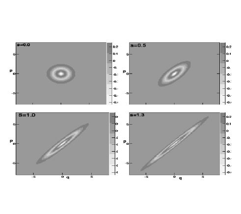
Figure 7: Contour plots of the Wigner functions of the squeezed Fock states $|0,s\exp(i\pi/6),3\rangle$ labeled by the squeezing strengths $s$. Irrespectively of $s$ the indicator $\delta\approx 0.97$.

V Concluding remarks

In this work we have proposed a simple indicator of non-classicality which measures the volume of the negative part of the Wigner function. Although the proposed coefficient $\delta$ is a function of the related quantity $\nu$, recently introduced by Benedict, Czirják et al. BC99 ; FCM02 , it is much easier to compute numerically.

The quantity (2) was used to analyze exemplary quantum states, including the Schrödinger cat states. The nonclassicality $\delta$ increases with the separation between the classical points defining the cat state. This growth saturates, if the separation distance is so large that the quantum interference patterns are well isolated from both main peaks of the distributions. Moreover, for a non–zero momentum $p_{0}\neq 0$, the quantity $\delta$ undergoes oscillations until the separation distance becomes so large that both packets are separated from the interference patterns. Asymptotically, if the separation is large enough, the indicator $\delta$ does not depend on $p_{0}$ and tends to a constant value, $\delta_{max}\approx 0.636$.

In the case of Fock states $|n\rangle$, the quantity $\delta$ equals zero for the coherent vacuum state $|0\rangle$ and grows monotonically with the quantum number $n$. If a quantum state is displaced by the Glauber operator $D(\beta)$, the shape of the Wigner function and the nonclassicality parameter do not change. Although the squeezing operator $S(\eta)$ changes the shape of the Wigner function, our results obtained for the squeezed Fock states show that the nonclassicality $\delta$ does not depend on squeezing.

The results presented in this work were obtained for pure states of infinite dimensional Hilbert space with use of the standard harmonic oscillator coherent states. It is worth to emphasize that our approach is also suited to analyze mixed quantum states. Furthermore, one may study the similar problem for quantum states of a finite dimensional Hilbert space, which was originally tackled in BC99 . In such a case one defines the Husimi function with the help of the $SU(2)$, spin coherent states, while the Wigner functions may be obtained by expanding the density matrix in the complete basis of the rotation operators Ag81 ; DAS94 ; HW00 . The Wigner function for finite dimensional systems may also be defined in alternative ways - see Wo87 ; GTP88 ; VP90 ; Le95 ; MKI01 ; MCS03 ; Wo03 and references therein. Studying the volume of the negative part of the Wigner function, defined according to any of these approaches, one may get an interesting information concerning the nonclassical properties of the state analyzed. For instance some recent attempts Ga04 ; DMWS04 ; Be04 try to link the negativity of the Wigner function with the entanglement of analyzed quantum states defined on a composed Hilbert space, or with the violation of the Bell inequalities.

VI Acknowledgment

We are indebted to I. Białynicki–Birula, I. Bengtsson, J. Burgdörfer, A.R.R. Carvalho, E. Galvão, A. Miranowicz, A.M. Ozorio de Almeida, J. M. Rost, K. Rza̧żewski and M.S. Santhanam for fruitful discussions, comments and remarks. We also would like to thank P.W. Schleich for helpful correspondence and several remarks that allowed us to improve the manuscript. Financial support by Polish Ministry of Scientific Research under the grant No PBZ-Min-008/P03/2003 and the VW grant ’Entanglement measures and the influence of noise’ is gratefully acknowledged. AK gratefully acknowledges the financial support by Alexander von Humboldt (AvH) Foundation/Bonn-Germany, under the grant of Research fellowship No.IV.4-KAM 1068533 STP.

References

- (1) L. Mandel, Opt. Lett. 4 (1979) 205
- (2) V.V Dodonov, J. Opt. B. - Quantum. Semiclss. O. 4 (2002) R1
- (3) M. Hillery, Phys. Rev. A 35 (1987) 725.
- (4) M. Hillery, Phys. Rev. A 39 (1989) 2994.
- (5) V.V Dodonov, O.V. Man’ko, V.I. Man’ko, A. Wünsche J. Mod. Opt. 47 (2000) 633.
- (6) V.V. Dodonov and M.B. Renó, Phys. Lett. A 308 (2002) 249.
- (7) P. Marian, T. A. Marian, and H. Scutaru, Phys. Rev. Lett. 88, (2002) 153601.
- (8) P. Marian, T. A. Marian and H. Scutaru, Phys. Rev. A 68 (2003) 062309
- (9) A. T. Avelar, B. Baseia and J. M. C. Malbouisson, preprint quant-ph/0308161 (2003).
- (10) K. Życzkowski and W. Słomczyński J. Phys. A 31 (1998) 9055
- (11) K. Życzkowski and W. Słomczyński J. Phys. A 34 (2001) 6689.
- (12) K.E. Cahill and R.J. Glauber, Phys. Rev. 177, (1969) 1882;
- (13) C. T. Lee, Phys. Rev. A 44 (1991) R2775.
- (14) C. T. Lee Phys. Rev. A 45 (1992) 6586.
- (15) N. Lütkenhaus and S. M. Barnett, Phys. Rev. A 51 (1995) 3340.
- (16) M.A. Marchiolli, V.S. Bagnato, Y. Guimaraes and B. Baseia, Phys. Lett. A 279 (2001) 294.
- (17) J. M. C. Malbouisson and B. Baseia, Physica Scripta 67 (2003) 93.
- (18) A. J. Bracken, H.-D. Doebner and J. G. Wood, Phys. Rev. Lett 83 (1999) 3758
- (19) G. Manfredi and M. R. Feix, Phys. Rev. E 62 (2000) 4665
- (20) J. J. Włodarz, Int. J. Theor. Phys. 42 (2003) 1075
- (21) R. L. Hudson, Rep. Math. Phys. 6 (1974) 249.
- (22) J.S. Bell, Speakable and unspeakable in quantum mechanics, Cambridge Univ. Press (1987), 196-200
- (23) A. Einstein, B. Podolsky and N. Rosen, Phys.Rev.47 (1935) 777
- (24) K. Banaszek and K. Wódkiewicz, Phys.Rev.A58 (1998) 4345
- (25) O. Cohen, Phys.Rev.A56 (1997) 3484.
- (26) K. Banaszek and K. Wódkiewicz, Acta.Phys.Slovaca 49 (1999) 491
- (27) K. Banaszek and K. Wódkiewicz, Phys.Rev.Lett.82 (1999) 2009
- (28) D. T. Smithey, M. Beck, M. G. Raymer and A. Faridani Phys. Rev. Lett. 70 (1993) 1244; T. J. Dunn, I. A. Walmsley and S. Mukamel, Phys. Rev. Lett. 74 (1995) 884; G. Breitenbach, S. Schiller and J. Mlynek, Nature 387 (1997) 471; K. Banaszek, C. Radzewicz and K. Wódkiewicz, Phys. Rev. A 60 (1999) 674
- (29) Ch. Kurtsiefer, T. Pfau and J. Mlynek, Nature 386 (1997) 150; G. Nogues, A. Rauschenbeutel, S. Osnaghi, P. Bertet, M. Brune, J. M. Raimond, S. Haroche, L.G. Lutterbach and L. Davidovich, Phys. Rev. A 62, (2000) 054101; A. I. Lvovsky, H. Hansen, T. Aichele, O. Benson, J. Mlynek and S. Schiller, Phys. Rev. Lett. 87 (2001) 0504021.
- (30) P. Lougovski, E. Solano, Z. M. Zhang, H. Walther, H. Mack and P. Schleich, Phys. Rev. Lett. 91 (2003) 0104011; W. E. Lamb, Phys. Today 22 (1969) 23; K. Wódkiewicz, Phys. Rev. Lett. 52 (1984) 1064; A. Royer, Phys.Rev.Lett.55 (1985) 2745; K. Banaszek and K. Wódkiewicz, Phys. Rev. Lett. 76 (1996) 4344.
- (31) U. Leonhardt, Measuring the Quantum State of Light, Cambridge Univ. Press, (1997)
- (32) E.P. Wigner, Phys. Rev. 40 (1932) 749
- (33) M. Hillery, R. F. O’Connell, M. O. Scully and E. P. Wigner, Phys. Rep. 106 (1984) 123
- (34) W. P. Schleich Quantum Optics in Phase Space, Wiley-VCH, Weinheim, (2001)
- (35) I. Białynicki–Birula, M. A. Cirone, J. P. Dahl, M. Fedorov and W. P. Schleich, Phys. Rev. Lett. 89 (2002) 0604041
- (36) J. P. Dahl, H. Mack, A. Wolf and W. P. Schleich, preprint, Ulm 2004
- (37) M.G. Benedict and A. Czirják, Phys. Rev. A.60 (1999) 4034.
- (38) P. Földi, A. Czirják, B. Molnár and M.G. Benedict, Opt. Express 10 (2002) 376.
- (39) L. Mandel and E. Wolf, Optical Coherence and Quantum Optics, Cambridge University Press, 1995.
- (40) G. M. Abd Al-Kader J. Opt. B: Quantum Semiclass. Opt.5 (2003) S228
- (41) G. S. Agarwal, Phys. Rev. A 24 (1981) 2889.
- (42) J. P. Dowling, G.S. Agarwal and W. P. Schleich, Phys. Rev. A 49 (1994) 4101.
- (43) S. Heiss and S. Weigert, Phys. Rev. A 63 (2000) 012105.
- (44) W. K. Wootters, Ann. Phys. 176, 1 (1987); K. S. Gibbons, M. J. Hoffman and W. K. Wootters, preprint quant-ph/0401155 (2004).
- (45) D. Galetti and A. F. R. De Toledo Piza, Physica A 149 (1988) 267.
- (46) J. A. Vaccaro and D. T. Pegg, Phys. Rev. A 41 (1990) 5156.
- (47) U. Leonhardt, Phys. Rev. Lett. 74 (1995) 4101.
- (48) A. Miranowicz, W. Leoński, and N. Imoto, Adv. Chem. Phys. 119 (2001) 155.
- (49) N. Mukunda, S. Chaturvedi, and R. Simon, Phys.Lett.A 321 (2004) 160
- (50) W. K. Wootters, IBM J. Res. Dev. 48 (2004) 99
- (51) E. Galvão, preprint quant-ph/0405070 (2004)
- (52) I. Bengtsson, preprint, Stockholm, 2004