Casimir Force between a Small Dielectric Sphere and a Dielectric Wall

Abstract

The possibility of repulsive Casimir forces between small metal spheres and a dielectric half-space is discussed. We treat a model in which the spheres have a dielectric function given by the Drude model, and the radius of the sphere is small compared to the corresponding plasma wavelength. The half-space is also described by the same model, but with a different plasma frequency. We find that in the retarded limit, the force is quasi-oscillatory. This leads to the prediction of stable equilibrium points at which the sphere could levitate in the Earth’s gravitational field. This seems to lead to the possibility of an experimental test of the model. The effects of finite temperature on the force are also studied, and found to be rather small at room temperature. However, thermally activated transitions between equilibrium points could be significant at room temperature.

I Introduction

The interaction energy between a particle with non-dispersive polarizability $\alpha_{0}$ and a perfectly reflecting wall was found by Casimir and Polder Polder to be

$$V_{CP}=-\frac{3\alpha_{0}}{32\pi^{2}z^{4}},$$ (1)

where $z$ is the separation. One can assign a frequency spectrum $\hskip 0.72229pt\sigma(\omega)$ to this potential and write Ford98

$$V_{CP}=\frac{\alpha_{0}}{16\pi^{2}z^{3}}\int_{0}^{\infty}d\omega\hskip 0.72229pt\sigma(\omega),$$ (2)

where

$$\sigma(\omega)=(2\omega^{2}z^{2}-1)\sin 2\omega z+2\omega z\cos 2\omega z.$$ (3)

The integrand, $\sigma(\omega)$, is an oscillatory function whose amplitude increases with increasing frequency. Nonetheless, the integral can be performed using a convergence factor (e.g., insert a factor of $e^{-\gamma\omega}$ and then let $\gamma\rightarrow 0$ after integration). The result is the right hand side of Eq. (1). It is clear that massive cancellations have occurred, and that the area under an oscillation peak can be much greater in magnitude than the final result. This raises the possibility of tampering with this delicate cancellation, and dramatically altering the magnitude and sign of the force.

In an earlier paper Ford98 , henceforth I, this possibility was investigated for small dielectric spheres near a perfectly reflecting wall. There it was found that the force can be considerably larger than that given by Eq. (1), and furthermore can be either attractive or repulsive. The force was found to be quasi-oscillatory, with a period of the order of the plasma wavelength of the material in the sphere. This effect can be understood as a resonance phenomenon involving the vacuum modes and the plasma frequency of the sphere. The calculations in I were restricted to the case of a perfectly reflecting wall at zero temperature. In the present paper, we generalize these results to the cases when the wall has finite reflectivity and the temperature is non-zero.

In Sect. II, a force on a small sphere near a dielectric wall is computed at zero temperature. In Sect. III, finite temperature corrections are discussed. The results of the papers are summarized in Sect. IV.

II Force on a Small Sphere near a Dielectric Wall

A small sphere of radius $a$ is placed a distance $z$ from a wall. Both the sphere and the wall are composed of uniform material characterized with dielectric function $\epsilon(\omega)$. We will take the dielectric function to be that of the Drude model,

$$\epsilon(\omega)=1-\frac{\omega_{p}^{2}}{\omega(\omega+i\gamma)},$$ (4)

where $\omega_{p}$ is the plasma frequency and $\gamma$ is the damping parameter. From now on, we take $\omega_{p}$ to be the plasma frequency of the material in the sphere, and $\omega_{q}$ to be that of the interface. We will use subscripts $w$ and $s$ to distinguish between other parameters describing the wall and the sphere respectively. At present, we assume that the temperature is zero.

The mean Casimir force on the sphere can be written as a Fourier transform:

$$\mathbf{F}=\frac{1}{2\pi}\int d\omega\,\mathbf{F}(\omega),$$ (5)

where $\mathbf{F}(\omega)$ can be viewed as the contribution of a vacuum mode of frequency $\omega$. This contribution can be found from essentially classical considerations, as it is the normal component of the classical force on the sphere when a plane wave of frequency $\omega$ is incident on the sphere-interface system. In I, it was calculated in an electric dipole approximation for the wave scattered by the sphere; the force is found as an integral of the Maxwell stress tensor over the sphere. In the present case, the extra complications come from the finite reflectivity of the interface. However, these can be handled using the dyadic Green’s function techniques of Schwinger et al Milton .

The result for $\mathbf{F}$ (or $V$) follows from

$$\mathbf{F}(\omega)=-\frac{1}{2}\nabla\alpha_{r}(\omega)\left\langle E^{2}\right\rangle_{\omega},$$ (6)

where $\left\langle E^{2}\right\rangle$ is the (renormalized) expectation value of the square of the electric field at the sphere’s location and $\alpha_{r}(\omega)$ is the real part of the dynamic polarizability. This expression is equivalent to the familiar result that the interaction energy of an induced dipole with a static electric field $E_{0}$ is

$$V=-\frac{1}{2}\alpha_{0}E_{0}^{2},$$ (7)

where $\alpha_{0}$ is the static polarizability of the particle. It turns out that this expression can be applied to the dynamic case as well, e.g. by expressing $\left\langle E^{2}\right\rangle_{\omega}$ in Eq. (6) as a transverse spatial Fourier transform Vasilka :

$$\left\langle E^{2}\right\rangle_{\omega}=-{\rm Re}\left\{i\int(d\mathbf{k}_{\perp})\,\frac{1}{(2\pi)^{2}}\frac{1}{2\kappa}\left[\omega^{2}r+\left(2k^{2}-\omega^{2}\right)r^{\prime}\right]e^{-2\kappa z}\right\}\,.$$ (8)

where $\mathbf{k}_{\perp}$ is the transverse wavevector, and $k=\left|\mathbf{k}_{\perp}\right|$. The reflection coefficients due to two polarization states of the electric field vector, $r$ and $r^{\prime}$, are given by:

$$r \equiv \frac{\kappa-\kappa_{1}}{\kappa+\kappa_{1}},$$ (9)

$$r^{\prime} \equiv \frac{\kappa\epsilon_{w}-\kappa_{1}}{\kappa\epsilon_{w}+\kappa_{1}},$$ (10)

where $\kappa$ is defined by $\kappa^{2}=k^{2}-\omega^{2}$, and $\kappa_{1}$ by $\kappa_{1}^{2}=k^{2}-\omega^{2}\epsilon_{w}.$

A detailed discussion is given in the Appendix, but the result for the interaction potential ($\mathbf{F}=-\nabla V$) can be written as

$$V={\rm Re}\left\{\frac{i}{4\pi}\int_{-\infty}^{\infty}d\omega\,\alpha_{r}\int_{0}^{\infty}dkk\frac{1}{2\pi}\frac{1}{2\kappa}\left[\omega^{2}r+\left(2k^{2}-\omega^{2}\right)r^{\prime}\right]e^{-2\kappa z}\right\}\,.$$ (11)

This is similar to Eq. (3.34) in Ref. Milton , which gives the interaction energy between a molecule and a dielectric plate. In our case, the molecule has been replaced by a dielectric sphere, and the polarizability of the sphere $\alpha$ has been replaced by its real part, $\alpha_{r}$. This is also a generalization of Eq. (45) in I. The treatment in I assumed no evanescent modes. However, the quantization of the electromagnetic field in the presence of a dissipative dielectric requires one to treat the frequency $\omega$ and wave number $k$ as independent variables, effectively leading to evanescent wave contributions. A detailed justification for the use of the real part of the dynamic polarizability, $\alpha_{r}$, was given in I.

The complex polarizability of the sphere is given by

$$\alpha(\omega)=\alpha_{0}\frac{\epsilon_{s}(\omega)-1}{\epsilon_{s}(\omega)+2},$$ (12)

where $\alpha_{0}$, the static polarizability, is given by $\alpha_{0}=4\pi a^{3}$. If $\epsilon_{s}(\omega)$ is given by the Drude model, Eq. (4), then the real part of the polarizability is

$$\alpha_{r}=\alpha_{0}\,\omega_{p}^{2}\frac{\omega_{p}^{2}-3\omega^{2}}{(3\omega^{2}-\omega_{p}^{2})^{2}+9\omega^{2}\gamma_{s}^{2}}.$$ (13)

This function has four poles in the complex $\omega$-plane, at $\pm\Omega\pm i\gamma_{s}/2$, where

$$\Omega=\frac{1}{6}\sqrt{12\omega_{p}^{2}-9\gamma_{s}^{2}}\,.$$ (14)

It will be convenient to deform the contour of integration in the $\omega$-plane, and isolate the residues of these poles. However, we must first consider the location of other possible singularities of the integrand of Eq. (11). There are branch points at the values of $\omega$ for which $\kappa=0$ and $\kappa_{1}=0$. The former occur at $\omega=\pm k$. The latter are in the lower half $\omega$-plane. In the limit that $\gamma_{w}\ll\omega_{q}$, they are located at approximately

$$\omega=\pm\sqrt{\omega_{q}^{2}+k^{2}}-i\,\frac{\gamma_{w}\,\omega_{q}^{2}}{2\,(\omega_{q}^{2}+k^{2})}\,.$$ (15)

The dielectric function $\epsilon_{w}(\omega)$ has a pole at $\omega=-i\gamma_{w}$, but both of the reflection coefficients, $r$ and $r^{\prime}$, are regular at this point. Finally, there is a possibility of poles in the reflection coefficients at points at which $\kappa=-\kappa_{1}$ or $\epsilon\,\kappa=-\kappa_{1}$. However, it may be shown that no such points exist. The electric field Green’s function should be defined by an integration contour which goes beneath the singularities for ${\rm Re}\,\omega<0$ and above them for ${\rm Re}\,\omega>0$, that is, Feynman boundary conditions. However, this does not include the poles of $\alpha_{r}(\omega)$, which is not part of the electric field Green’s function. Thus the contour of integration is as illustrated in Fig. 1.

Figure 1: The contour of integration for Eq. (11) in the complex $\omega$-plane for fixed $k$ is illustrated. Here $X$ marks a branch point, and a dotted line is its associated branch cut. The poles of the function $\alpha_{r}(\omega)$ are marked with the $+$ symbol. When the contour is rotated to the imaginary axis, the poles in the first and third quadrants are the only singularities encountered.

We may now rotate the contour of integration to the imaginary $\omega$-axis, so that $V$ can be written as the sum of an integral over imaginary frequencies, $V_{j}$, and a contribution, $V_{p}$, from the residues of the pole in $\alpha_{r}$:

$$V=V_{j}+V_{p},$$ (16)

with

$$V_{j}=-\frac{1}{8\pi^{2}}\int_{0}^{\infty}d\zeta\alpha_{r}(i\zeta)\int_{0}^{\infty}dkk\frac{1}{\kappa}\left[-\zeta^{2}\overline{r}+\left(2k^{2}+\zeta^{2}\right)\overline{r^{\prime}}\right]e^{-2\kappa z},$$ (17)

and

$$V_{p}=\frac{\alpha_{0}\,\omega_{p}^{2}}{48\pi\Omega}\;{\rm Re}\int_{0}^{\infty}dkk\frac{1}{\kappa(\omega_{1})}\left[\omega_{1}^{2}\,\overline{r}(\omega_{1})+\left(2k^{2}-\omega_{1}^{2}\right)\overline{r^{\prime}}(\omega_{1})\right]e^{-2\kappa(\omega_{1})z},$$ (18)

where $\omega_{1}$ is the pole of $\alpha_{r\text{ }}$in the first quadrant,

$$\omega_{1}=\frac{1}{6}\sqrt{12\omega_{p}^{2}-9\gamma_{s}^{2}}+\frac{1}{2}i\gamma_{s},$$ (19)

and $\overline{r}$ is defined as

$$\overline{r}=\frac{r(\gamma_{w})+r(-\gamma_{w})}{2},$$ (20)

and similarly for $\overline{r^{\prime}}$. The first term in Eq. (20) arises from the pole in the first quadrant, and the second term from that in the third quadrant, and we have used the fact that the Drude model dielectric function satisfies $\epsilon(-\omega,\gamma)=\epsilon(\omega,-\gamma)$.

By introducing polar coordinates $u$ and $\theta$ ( $\zeta=u\cos\theta,$ $k=u\sin\theta$ ), and subsequently taking $t\equiv\cos(\theta)$, Eq. (17) becomes

$$V_{j}=-\alpha_{0}\frac{\omega_{p}^{2}}{8\pi^{2}}\int_{0}^{\infty}du\int_{0}^{1}dt\frac{3u^{2}t^{2}+\omega_{p}^{2}}{(3u^{2}t^{2}+\omega_{p}^{2})^{2}-9u^{2}t^{2}\gamma_{s}^{2}}u^{3}\;{\rm Re}\left[-t^{2}\overline{r}+\left(2-t^{2}\right)\overline{r^{\prime}}\right]e^{-2uz}.$$ (21)

The numerical evaluation of the integral is done in the limit $\gamma_{s}\rightarrow 0$, $\gamma_{w}\rightarrow 0$ (plasma model regime). In this case we can write the coefficients $r$ and $r^{\prime}$ (in place of $\overline{r}$ and $\overline{r^{\prime}}$) , as defined in Eq. (10), in terms of the new variables as

$$r = \frac{u-\sqrt{u^{2}+\omega_{q}^{2}}}{u+\sqrt{u^{2}+\omega_{q}^{2}}},$$ (22)

$$r^{\prime} = \frac{u^{2}t^{2}+\omega_{q}^{2}-ut^{2}\sqrt{u^{2}+\omega_{q}^{2}}}{u^{2}t^{2}+\omega_{q}^{2}+ut^{2}\sqrt{u^{2}+\omega_{q}^{2}}}.$$ (23)

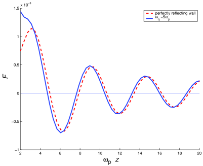
Figure 2: The force, in units of $\omega_{p}^{5}\,\alpha_{0}$, is given for the case $\omega_{q}=5\omega_{p}$. Repulsion corresponds to $F>0$. Here the result is quite close to that for the perfectly reflecting wall (dashed line).

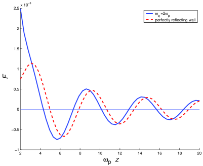
Figure 3: The force is given for the case $\omega_{q}=2\omega_{p}$. Here the finite reflectivity has caused a shift in the locations of the force maxima and minima, but little change of the magnitude of the maximum force.

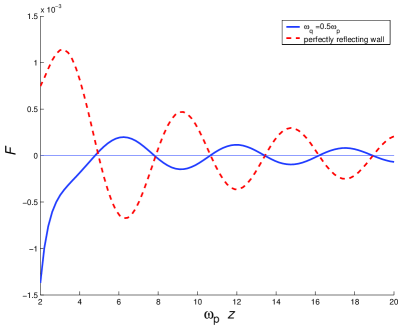
Figure 4: The force is given for the case $\omega_{q}=0.5\omega_{p}$. Besides a shift in the locations of the force maxima and minima, the finite reflectivity has caused a reduction in the magnitude of the maximum force.

In Figures 2 - 4, the force on the sphere ($\mathbf{F}=-\nabla\left(V_{j}+V_{p}\right)$) in units $\omega_{p}^{5}\,\alpha_{0}$ is given for three different ratios $\omega_{q}/\omega_{p}$. The $V_{p}$ term is typically dominant, and gives rise to a quasi-oscillatory contribution to the force, as seen in the figures. This quasi-oscillatory behavior is in contrast to the monotonic attractive force in the case of an atom in its ground state interacting with an interface Polder , Milton . However, it is similar to the force between an atom in an excited state and an interface Barton , which is also quasi-oscillatory. In the present case, the oscillations arise from a resonance at $\omega=\omega_{1}\approx\sqrt{3}\omega_{p}/3$, if $\gamma_{s}\ll\omega_{p}$, as seen from Eq. (19). The appearance of the real part of the polarizability is crucial for this feature of the result. The force is alternatively attractive and repulsive as a function of separation, and this leads to a sequence of stable equilibrium positions for the sphere. These are the zeros of the function $\mathbf{F}(z)$ with negative slope. This seems to lead to the possibility of an experimental test of the model in which the sphere could levitate in the Earth’s gravitational field at positions where $\mathbf{F}$ cancels the sphere’s weight, as discussed in I. Note that $F$ is defined so that $F>0$ is repulsion, and $F<0$ is attraction. Also note that because the present paper adopts Lorentz-heaviside units, in contrast to the Gaussian units used in I, the scale in the figures differs by a factor of $4\pi$ from Fig. 7 in I.

Of particular interest is the effect of the finite reflectivity of the interface, which is described by its plasma frequency, $\omega_{q}$. As expected, when $\omega_{q}\gg\omega_{p}$, the results agree with those given in I for a perfectly reflecting wall. As the ratio $\omega_{q}/\omega_{p}$ decreases, the force oscillations shift their phase and eventually decrease in amplitude, as seen in the figures. In Figure 2 we see that if $\omega_{q}$ is larger than a few times $\omega_{p}$, the perfectly conducting result is a very good approximation (dashed line). Even when $\omega_{q}<\omega_{p}$, as in Figure 4, one still finds the quasi-oscillatory behavior of the force. The amplitude of the force decreases, as expected, since the effect should disappear as $\omega_{q}\rightarrow 0$.

In the small distance limit, $a\ll z\ll\omega_{p}^{-1}$, the expression for the total force on the particle in the plasma model regime becomes

$$\mathbf{F}=-\frac{d}{dz}(V_{j}+V_{p})\approx-\frac{\alpha_{0}}{4\pi}\frac{3\sqrt{2}}{8}\frac{\omega_{p}^{2}\omega_{q}}{2\omega_{p}^{2}-3\omega_{q}^{2}}\frac{1}{z^{4}}.$$ (24)

We see that the force diverges near the interface, and moreover its sign depends on the ratio $\omega_{p}/\omega_{q}$, which seems to be an artifact of the assumption of a perfectly smooth interface. As discussed in Ref. Vasilka , dispersion alone is not sufficient to render mean squared electromagnetic fields finite in the limit that one approaches such an interface.

II.1 Perfectly reflecting Wall

In the limit $\epsilon_{w}\rightarrow\infty$, as seen from (9) and (10), $r\rightarrow-1$ , and $r^{\prime}\rightarrow 1$ . In this case (21) can be analytically integrated over $t$ yielding:

$$V_{j}= \alpha_{0}\frac{\omega_{p}^{2}}{4\pi^{2}}\frac{1}{\sqrt{3}\sqrt{4\omega_{p}^{2}-3\gamma_{s}^{2}}}\int_{0}^{\infty}du\,u^{2}$$ (25)

$$\times \left[\arctan\left(\frac{\sqrt{3}\left(-2u+\gamma_{s}\right)}{\sqrt{4\omega_{p}^{2}-3\gamma_{s}^{2}}}\right)-\arctan\left(\frac{\sqrt{3}\left(2u+\gamma_{s}\right)}{\sqrt{4\omega_{p}^{2}-3\gamma_{s}^{2}}}\right)\right]e^{-2uz},$$

and (18), after analytical evaluation, becomes:

$$V_{p}=-\frac{\alpha_{0}}{4\pi}\frac{\omega_{p}^{2}}{24\Omega}\frac{1}{z^{3}}\left(2\omega_{1}^{2}z^{2}+2i\omega_{1}z-1\right)e^{2i\omega_{1}z}.$$ (26)

It can be shown that these results agree with the ones in I, namely we find that the total force on the sphere in this limit becomes:

$$F=J+P,$$ (27)

where

$$J=-\frac{d}{dz}V_{j}=-\alpha_{0}\frac{\omega_{p}^{2}}{16\pi^{2}z^{4}}\int_{0}^{\infty}d\xi\frac{\left(3\xi^{2}+\omega_{p}^{2}\right)\left(4z^{3}\xi^{3}+6z^{2}\xi^{2}+6z\xi+3\right)}{\left(3\xi^{2}+\omega_{p}^{2}\right)^{2}-9\xi^{2}\gamma_{s}^{2}}e^{-2z\xi},$$ (28)

and

$$P = {\rm Re}\left(-\frac{d}{dz}V_{p}\right)$$ (29)

$$= -\alpha_{0}\frac{\omega_{p}^{2}}{192\pi\Omega}\frac{1}{z^{4}}e^{-\gamma_{s}z}\left[2\Omega z\left(4\Omega^{2}z^{2}-3\gamma_{s}^{2}z^{2}-6\gamma_{s}z-6\right)\sin 2\Omega z+\right.$$

$$\left.\left(12\gamma_{s}\Omega^{2}z^{3}-\gamma_{s}^{3}z^{3}+12\Omega^{2}z^{2}-3\gamma_{s}^{2}z^{2}-6\gamma_{s}z-6\right)\cos 2\Omega z\right]\,.$$

As seen here, the plasma model is a good approximation as long as $\gamma_{s}z\ll 1$. Otherwise, Eq. (29) can yield significant corrections for the more distant equilibrium positions, but not for the first several peaks. We expect this to be true for the case of finite conductivity of the wall as well, as long as $\gamma_{s}\ll\omega_{p}$, and $\gamma_{w}\ll\omega_{q}$.

III Finite Temperature Corrections

In the case of nonzero temperature, Eqs. (17) and (18) have to be modified. We write Eq. (17) as a Fourier series instead of Fourier transform by the substitution Milton

$$\zeta^{2}\rightarrow\zeta_{n}^{2}=\frac{4\pi^{2}n^{2}}{\beta^{2}},\qquad\int_{0}^{\infty}\frac{d\zeta}{2\pi}\longrightarrow\frac{1}{\beta}\sum_{n=0}^{\infty}{}^{\prime}.$$ (30)

The prime is a reminder to count the $n=0$ term with half weight, and $\beta=1/kT$. Thus, in the limit $\gamma_{s},\gamma_{w}\approx 0$:

$$V_{j}=-\frac{\alpha_{0}\omega_{p}^{2}}{4\pi\beta}\;{\rm Re}\sum_{n=0}^{\infty}{}^{\prime}\frac{1}{3\zeta_{n}^{2}+\omega_{p}^{2}}\int_{0}^{\infty}\frac{dk\,k}{\kappa}\left[-\zeta_{n}^{2}r+\left(2k^{2}+\zeta_{n}^{2}\right)r^{\prime}\right]e^{-2\kappa z},$$ (31)

where $r$ and $r^{\prime}$, using Eqs. (9), (10) and (4) can be written as:

$$r \equiv \frac{\kappa-\sqrt{\kappa^{2}+\omega_{q}^{2}}}{\kappa+\sqrt{\kappa^{2}+\omega_{q}^{2}}},$$ (32)

$$r^{\prime} \equiv \frac{\kappa\left(\zeta_{n}^{2}+\omega_{q}^{2}\right)-\zeta_{n}^{2}\sqrt{\kappa^{2}+\omega_{q}^{2}}}{\kappa\left(\zeta_{n}^{2}+\omega_{q}^{2}\right)+\zeta_{n}^{2}\sqrt{\kappa^{2}+\omega_{q}^{2}}}.$$ (33)

We modify Eq. (18) by inserting a factor $\left(1+\frac{2}{e^{\beta\omega}-1}\right)$ to account for the thermal energy. This factor reflects the fact that at zero temperature, each mode has an energy of $\frac{1}{2}\omega$; at finite temperature, there is an additional thermal energy of $1/\left(e^{\beta\omega}-1\right)$. The result is

$$V_{p}=\frac{\alpha_{0}\,\omega_{p}^{2}}{24\pi\Omega}\;{\rm Re}\left\{\left(\frac{1}{e^{\beta\omega_{1}}-1}+\frac{1}{2}\right)\int_{0}^{\infty}dkk\frac{1}{\kappa(\omega_{1})}\left[\omega_{1}^{2}r(\omega_{1})+\left(2k^{2}-\omega_{1}^{2}\right)r^{\prime}(\omega_{1})\right]e^{-2\kappa(\omega_{1})z}\right\}\,.$$ (34)

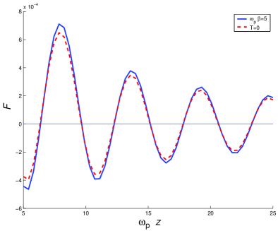
Figure 5: The force is given for the case $\omega_{q}=\omega_{p}$ and $\omega_{p}\beta=5$. The effect of the finite temperature is a slight increase in the magnitude of the force.

The electric dipole approximation requires that the radius of the sphere be small compared to the dominant wavelengths involved, so our results require that $a\ll\beta$. So long as the temperature stays within this range of validity, the thermal correction enhances the magnitude of the force, with no shift in the positions of the force maxima and minima as illustrated in Figure 5 for case $\omega_{p}\beta=5$. In most of the cases of interest, $\omega_{p}$ is in the ultraviolet range, so $\omega_{p}\beta\gg 1$ at room temperature. The temperature is also limited by the melting point of the material of the wall.

Although the finite-temperature corrections to the force are small, there is another thermal effect which can be more significant. This is the possibility of thermally activated transitions between the stable equilibrium points, which become important when the required energy is of order $kT$. We can estimate this effect by noting that for the case $\omega_{q}=2\omega_{p}$, this energy is approximately

$$W=\int_{4/\omega_{p}}^{7/\omega_{p}}f\,dz\approx 1.4\times 10^{-3}\,\alpha_{0}\,\omega_{p}^{4}\,,$$ (35)

which can be expressed as

$$W=2200K\left(\frac{a}{20nm}\right)^{3}\left(\frac{\omega_{p}}{10eV}\right)^{4}=280K\left(\frac{a}{10nm}\right)^{3}\left(\frac{\omega_{p}}{10eV}\right)^{4}\,.$$ (36)

Note that $10eV=1/20nm$, so for $\omega_{p}\approx 10eV$ the upper limit on the size of a sphere that would fit inside of a particular potential minimum is about $20nm$. In this case, the thermal activation effect would be small at room temperature. However, for a smaller sphere, e.g., $a=10nm$, thermal activation would be noticeable at room temperature.

IV Summary

We have investigated a model for the amplification of vacuum fluctuations, in which a resonance near the plasma frequency significantly increases the magnitude of the force compared to the non-dispersive case. In particular, we have examined the effects of finite reflectivity of the wall and of finite temperature. Finite reflectivity can decrease the magnitude of the effect, but so long as $\omega_{q}$ is of the order of, or larger than $\omega_{p}$, the perfectly reflecting results are qualitatively correct. Finite temperature can enhance the magnitude of the effect, but with typical plasma frequencies in the ultraviolet range, the correction to the force at room temperature is extremely small. However, thermal activation can be significant, especially for smaller spheres.

The key prediction of this model is a force that is alternatively attractive and repulsive as a function of separation. The ratio of the peak force to that of gravity on a sphere near an interface with $\omega_{q}>\omega_{p}$ is approximately given by

$$\frac{F_{max}}{F_{g}}\approx 27\,\left(\frac{\omega_{p}}{1eV}\right)^{4}\,\left(\frac{1\mu m}{z}\right)\,\left(\frac{1g/cm^{3}}{\rho}\right)\,e^{-5\,(\gamma_{s}/1eV)\,(z/1\mu m)}\,,$$ (37)

where $\rho$ is the mass density of the sphere. This suggests a possibility of an experimental test of the model in which the sphere could levitate in the Earth’s gravitational field at equilibrium positions. If forces whose magnitudes are large compared to those give by Eq. (1) with $\alpha_{0}\approx 4\pi a^{3}$ are found, the result can be interpreted as a form of amplification of vacuum fluctuations. The spheres need to be small ($a\omega_{p}\lesssim 1$), so experiments on metal sphere would have to involve spheres with radii in approximately the $10nm$ to $100nm$ range. In the case of gold spheres, for example, ($\omega_{p}=9eV$), the sphere radius would have to be less than $20nm$ and preferably less than about $10nm$.

One might also ask if a similar amplification is possible for the Casimir force between perfectly reflecting parallel plates. The spectrum of the Casimir force in this case was discussed by Hacyan, et al Hacyan , and one of the present authors Ford88 , and found to be quasi-oscillatory, as in the case of the Casimir-Polder potential. However, as was shown by Lifshitz Lifs , the force between a pair of dielectric half-spaces is always attractive and no larger in magnitude than the Casimir force. Thus upsetting the cancellation seems to be more difficult for half-spaces, and suggests that the small sphere approximation may be crucial. to obtain a quasi-oscillatory force. For larger objects, there may be a cancellation of the contributions of different spatial regions.

Appendix A Derivation for the Force on a small Sphere near a Wall

We can obtain Eq. (6) by using Eq. (11) in I as a starting point for the force on the sphere:

$$F^{i}=\frac{2}{3}p^{j}\partial_{j}E^{i}+\frac{1}{3}p_{j}\partial^{i}E^{j}+\frac{2}{3}\left(\dot{\mathbf{p}}\times\mathbf{B}\right)^{i},$$ (38)

where $\mathbf{p}$ is the dipole moment associated with the sphere, and $\mathbf{E}$ and $\mathbf{B}$ are the mean electric and magnetic field vectors at the sphere’s location. We take $\mathbf{p}$ to be linearly related to $\mathbf{E}$: $\mathbf{p=}\alpha\mathbf{E}$. Using the Maxwell equation, $\dot{\mathbf{E}}=\mathbf{\nabla}\times\mathbf{B}$, we get for the last term in Eq. (38):

$$\frac{2}{3}\left(\dot{\mathbf{p}}\times\mathbf{B}\right)^{i}=\frac{2}{3}\alpha\left[\left(\mathbf{\nabla}\times\mathbf{B}\right)\times\mathbf{B}\right]^{i}=\frac{2}{3}\alpha\left[-\left(\partial^{i}B^{k}\right)B_{k}+\left(\partial^{k}B^{i}\right)B_{k}\right].$$ (39)

Thus Eq. (38) becomes:

$$F^{i}=\frac{1}{3}\alpha\left[2E^{j}\partial_{j}E^{i}+E_{j}\partial^{i}E^{j}+2B_{j}\partial^{j}B^{i}-2B_{j}\partial^{i}B^{j}\right]$$ (40)

Now, we replace the field products with their appropriate expectation values for $i=z$. The expectation values of the electric and magnetic fields can be expressed through the Green’s dyadic as in Milton :

$$\frac{i}{\hbar}\left\langle E_{j}(\mathbf{r})\,E_{k}(\mathbf{r}^{\prime})\right\rangle=\Gamma_{jk}(\mathbf{r},\mathbf{r}^{\prime},\omega),$$ (41)

and

$$\frac{i}{\hbar}\left\langle B_{j}(\mathbf{r})\,B_{k}(\mathbf{r}^{\prime})\right\rangle=\epsilon_{jlm}\epsilon_{knp}(\partial_{l}\partial_{n}/\omega^{2}\,)\Gamma_{mp}(\mathbf{r},\mathbf{r}^{\prime},\omega).$$ (42)

Quantities such as $\langle E_{j}(\mathbf{r})\,E_{k}(\mathbf{r}^{\prime})\rangle$ must be real, so we need to take a real part, which will only be done explicitly in the final expressions. Some components of $\mathbf{\,}\overleftrightarrow{\mathbf{\Gamma}}$ are (here $\mathbf{k}_{\perp}$ is chosen to point along the $+x$ axis):

$$\Gamma_{xx}\mathbf{(\mathbf{r},\mathbf{r}^{\prime},}\omega\mathbf{)} = \mathbf{\int}d\mathbf{\mathbf{k}_{\bot}\;}\frac{1}{(2\pi)^{2}}e^{i\mathbf{k}_{\bot}(\mathbf{r}-\mathbf{r}^{\prime})_{\bot}}$$ (43)

$$\times \left[-\frac{1}{\epsilon}\delta(z-z^{\prime})+\frac{1}{\epsilon}\frac{\partial}{\partial z}\frac{1}{\epsilon^{\prime}}\frac{\partial}{\partial z^{\prime}}\left(\frac{e^{-\kappa\mid z-z^{\prime}\mid}+r^{\prime}e^{-\kappa(z+z^{\prime})}}{2\kappa}\right)\right],$$

$$\Gamma_{yy}\mathbf{(\mathbf{r},\mathbf{r}^{\prime},}\omega\mathbf{)} = \mathbf{\int}d\mathbf{\mathbf{k}_{\bot}\;}\frac{1}{(2\pi)^{2}}e^{i\mathbf{k}_{\bot}(\mathbf{r}-\mathbf{r}^{\prime})_{\bot}}\omega^{2}\left(\frac{e^{-\kappa\mid z-z^{\prime}\mid}+re^{-\kappa(z+z^{\prime})}}{2\kappa}\right),$$ (44)

$$\Gamma_{zz}\mathbf{(\mathbf{r},\mathbf{r}^{\prime},}\omega\mathbf{)} = \mathbf{\int}d\mathbf{\mathbf{k}_{\bot}\;}\frac{1}{(2\pi)^{2}}e^{i\mathbf{k}_{\bot}(\mathbf{r}-\mathbf{r}^{\prime})_{\bot}}$$ (45)

$$\times \left[-\frac{1}{\epsilon}\delta(z-z^{\prime})+\frac{k^{2}}{\epsilon\epsilon^{\prime}}\left(\frac{e^{-\kappa\mid z-z^{\prime}\mid}+r^{\prime}e^{-\kappa(z+z^{\prime})}}{2\kappa}\right)\right],$$

$$\Gamma_{xz}\mathbf{(\mathbf{r},\mathbf{r}^{\prime},}\omega\mathbf{)} = \mathbf{\int}d\mathbf{\mathbf{k}_{\bot}\;}\frac{1}{(2\pi)^{2}}e^{i\mathbf{k}_{\bot}(\mathbf{r}-\mathbf{r}^{\prime})_{\bot}}i\frac{k}{\epsilon\epsilon^{\prime}}\frac{\partial}{\partial z}\left(\frac{e^{-\kappa\mid z-z^{\prime}\mid}+r^{\prime}e^{-\kappa(z+z^{\prime})}}{2\kappa}\right),$$ (46)

$$\Gamma_{zx}\mathbf{(\mathbf{r},\mathbf{r}^{\prime},}\omega\mathbf{)} = \mathbf{\int}d\mathbf{\mathbf{k}_{\bot}\;}\frac{1}{(2\pi)^{2}}e^{i\mathbf{k}_{\bot}(\mathbf{r}-\mathbf{r}^{\prime})_{\bot}}\left(-i\right)\frac{k}{\epsilon\epsilon^{\prime}}\frac{\partial}{\partial z^{\prime}}\left(\frac{e^{-\kappa\mid z-z^{\prime}\mid}+r^{\prime}e^{-\kappa(z+z^{\prime})}}{2\kappa}\right).$$ (47)

Hence, for the first term in Eq. (40) we have:

$$i\left\langle E^{j}\partial_{j^{\prime}}E^{z}\right\rangle=\partial_{x^{\prime}}\Gamma^{xz}+\partial_{y^{\prime}}\Gamma^{yz}+\partial_{z^{\prime}}\Gamma^{zz}\,.$$ (48)

Next we drop the $\delta$-function terms, and take the coincidence limit, $\mathbf{r}^{\prime}=\mathbf{r}$ and $z^{\prime}=z$, after performing the $\partial_{j^{\prime}}$ differentiation. All derivatives in $y^{\prime}$ are zero, since $\mathbf{k}_{\perp}$ points along the $+x$ axis, so the second term above is zero. Using Eqs. (46) and (45), we find the remaining terms (with $\epsilon=\epsilon^{\prime}=1$ for the vacuum region):

$$\partial_{x^{\prime}}\Gamma^{xz} = -\frac{1}{2}\mathbf{\int}d\mathbf{\mathbf{k}_{\bot}\;}\frac{1}{(2\pi)^{2}}k^{2}\left(r^{\prime}e^{-2\kappa z}\pm 1\right),$$ (49)

$$\partial_{z^{\prime}}\Gamma^{zz} = -\frac{1}{2}\mathbf{\int}d\mathbf{\mathbf{k}_{\bot}\;}\frac{1}{(2\pi)^{2}}k^{2}\left(r^{\prime}e^{-2\kappa z}\mp 1\right)\,.$$ (50)

Here the sign of the last term is determined by whether $z$ approaches $z^{\prime}$ from above (upper sign) or from below (lower sign). We will argue later that these terms with ambiguous sign do not contribute to the final result. Now Eq. (48) becomes:

$$i\left\langle E^{j}\partial_{j^{\prime}}E^{z}\right\rangle=-\mathbf{\int}d\mathbf{\mathbf{k}_{\bot}\;}\frac{1}{(2\pi)^{2}}k^{2}r^{\prime}e^{-2\kappa z}.$$ (51)

For the second term in Eq. (40) we have:

$$i\left\langle E_{j}\partial^{z^{\prime}}E^{j}\right\rangle=\partial_{z^{\prime}}\left(\Gamma_{xx}+\Gamma_{yy}+\Gamma_{zz}\right).$$ (52)

Using Eqs. (43), (44), and (45), we can write:

$$\partial_{z^{\prime}}\Gamma_{xx} = -\frac{1}{2}\mathbf{\int}d\mathbf{\mathbf{k}_{\bot}\;}\frac{1}{(2\pi)^{2}}\kappa^{2}\left(r^{\prime}e^{-2\kappa z}\pm 1\right),$$ (53)

$$\partial_{z^{\prime}}\Gamma_{yy} = -\frac{1}{2}\mathbf{\int}d\mathbf{\mathbf{k}_{\bot}\;}\frac{1}{(2\pi)^{2}}\omega^{2}\left(re^{-2\kappa z}\mp 1\right),$$ (54)

$$\partial_{z^{\prime}}\Gamma_{zz} = -\frac{1}{2}\mathbf{\int}d\mathbf{\mathbf{k}_{\bot}\;}\frac{1}{(2\pi)^{2}}k^{2}\left(r^{\prime}e^{-2\kappa z}\mp 1\right),$$ (55)

so that Eq. (52) becomes:

$$i\left\langle E_{j}\partial^{z^{\prime}}E^{j}\right\rangle=-\frac{1}{2}\mathbf{\int}d\mathbf{\mathbf{k}_{\bot}\;}\frac{1}{(2\pi)^{2}}\left[\left(2k^{2}-\omega^{2}\right)r^{\prime}e^{-2\kappa z}+\omega^{2}re^{-2\kappa z}\mp 2\omega^{2}\right]\,.$$ (56)

For the third term in Eq. (40), we can write:

$$\left\langle B_{j}\partial^{j^{\prime}}B^{z}\right\rangle=\left\langle B_{x}\partial_{x^{\prime}}B_{z}\right\rangle+\left\langle B_{y}\partial_{y^{\prime}}B_{z}\right\rangle+\left\langle B_{z}\partial_{z^{\prime}}B_{z}\right\rangle.$$ (57)

The nonzero terms, using Eqs. (42) and (44), become:

$$i\left\langle B_{x}\partial_{x^{\prime}}B_{z}\right\rangle = -\frac{1}{2}\mathbf{\int}d\mathbf{\mathbf{k}_{\bot}\;}\frac{1}{(2\pi)^{2}}k^{2}\left(re^{-2\kappa z}\pm 1\right),$$ (58)

$$i\left\langle B_{z}\partial_{z^{\prime}}B_{z}\right\rangle = -\frac{1}{2}\mathbf{\int}d\mathbf{\mathbf{k}_{\bot}\;}\frac{1}{(2\pi)^{2}}k^{2}\left(re^{-2\kappa z}\mp 1\right),$$ (59)

So, Eq. (57) becomes:

$$i\left\langle B_{j}\partial^{j^{\prime}}B^{z}\right\rangle=-\frac{1}{2}\mathbf{\int}d\mathbf{\mathbf{k}_{\bot}\;}\frac{1}{(2\pi)^{2}}k^{2}\ 2re^{-2\kappa z}.$$ (60)

To find the fourth term in Eq. (40), note that Vasilka :

$$i\left\langle B_{j}B_{j}\right\rangle_{\omega}=\int\frac{d\mathbf{k}_{\perp}}{(2\pi)^{2}}$$ (61)

$$\times \left[\left(k^{2}+\nabla_{z}\nabla_{z^{\prime}}\right)\left(\frac{e^{-\kappa\mid z-z^{\prime}\mid}+re^{-\kappa(z+z^{\prime})}}{2\kappa}\right)+\omega^{2}\left(\frac{e^{-\kappa\mid z-z^{\prime}\mid}+r^{\prime}e^{-\kappa(z+z^{\prime})}}{2\kappa}\right)\right].$$

From here we get:

$$i\left\langle B_{j}\partial^{z^{\prime}}B^{j}\right\rangle=i\partial_{z^{\prime}}\left\langle B_{j}B_{j}\right\rangle=-\frac{1}{2}\mathbf{\int}d\mathbf{\mathbf{k}_{\bot}\;}\frac{1}{(2\pi)^{2}}\left\{\left[\left(2k^{2}-\omega^{2}\right)r+\omega^{2}r^{\prime}\right]e^{-2\kappa z}\mp 2\omega^{2}\right\}.$$ (62)

Combining Eqs. (51), (56), (60), and (62), as in Eq. (40), we have:

$$2\left\langle E^{j}\partial_{j^{\prime}}E^{z}\right\rangle+\left\langle E_{j}\partial^{z^{\prime}}E^{j}\right\rangle+2\left\langle B_{j}\partial^{j^{\prime}}B^{z}\right\rangle-2\left\langle B_{j}\partial^{z^{\prime}}B^{j}\right\rangle=$$

$${\rm Re}\left(\frac{i}{2}\mathbf{\int}d\mathbf{\mathbf{k}_{\bot}\;}\frac{1}{(2\pi)^{2}}\left\{3\left[\left(2k^{2}-\omega^{2}\right)r^{\prime}+\omega^{2}r\right]e^{-2\kappa z}\pm 2\omega^{2}\right\}\right)\,.$$ (63)

The last term above would give an infinite force and cannot be present. If we average over $z>z^{\prime}$ and $z<z^{\prime}$, it would average to zero. In the limit that $r=r^{\prime}=0$, the force must vanish, so we can drop the last term. Then, we let $\alpha\longrightarrow\alpha_{r}$, so that Eq. (40) becomes:

$$F^{z}(\omega)={\rm Re}\left\{\frac{i}{2}\mathbf{\int}d\mathbf{\mathbf{k}_{\bot}\;}\frac{1}{(2\pi)^{2}}\alpha_{r}(\omega)\left[\left(2k^{2}-\omega^{2}\right)r^{\prime}+\omega^{2}r\right]e^{-2\kappa z}\right\}$$ (64)

This is equivalent to Eq. (6), with $\left\langle E^{2}\right\rangle_{\omega}$ as defined in Eq. (8).

References

(1) H. B. G. Casimir and D. Polder, Phys. Rev. 73,
360 (1948).
(2) L.H. Ford, Phys. Rev. A. 58, 4279 (1998).
(3) J. Schwinger, L. L. DeRaad, and K. A. Milton, Ann. Phys.
(N.Y.) 115, 1 (1978).
(4) V. Sopova and L. H. Ford, Phys. Rev. D 66, 045026 (2002).
(5) J. Schwinger, Particles, Sources, and Fields,
Vols. I, II, (Addison-Wesley, Reading, Mass. 1970, 1973).
(6) G. Barton, Phys. Lett. B 237, 559 (1990).
(7) S. Hacyan, R. Jáuregui, F. Soto, and C. Villarreal, J.
Phys. A 23, 2401 (1990).