Casimir-Polder interaction between an atom and a cavity wall under the influence of real conditions
Abstract
The Casimir-Polder interaction between an atom and a metal wall is investigated under the influence of real conditions including the dynamic polarizability of the atom, finite conductivity of the wall metal and nonzero temperature of the system. Both analytical and numerical results for the free energy and force are obtained over a wide range of the atom-wall distances. Numerical computations are performed for an Au wall and metastable He∗, Na and Cs atoms. For the He∗ atom we demonstrate, as an illustration, that at short separations of about the Au plasma wavelength at room temperature the free energy deviates up to 35% and the force up to 57% from the classical Casimir-Polder result. Accordingly, such large deviations should be taken into account in precision experiments on atom-wall interactions. The combined account of different corrections to the Casimir-Polder interaction leads to the conclusion that at short separations the corrections due to the dynamic polarizability of an atom play a more important role than — and suppress — the corrections due to the nonideality of the metal wall. By the comparison of the exact atomic polarizabilities with those in the framework of the single oscillator model, it is shown that the obtained asymptotic expressions enable calculation of the free energy and force for the atom-wall interaction under real conditions with a precision of one percent.
pacs:
34.50.Dy, 12.20.Ds, 11.10.Ws, 34.20.CfI Introduction
The interactions of atoms with a single cavity wall have long been investigated in different physical, chemical and biological processes including adsorption and scattering from various surfaces1 . Due to high interest in nanotechnological applications of atoms near surfaces and mesoscopic scale atomic devices there is a need for accurate characterization of atom-surface interactions. Recent experimental studies include “quantum reflection” of ultracold metastable Ne atoms on Si or glass surfaces 2 and low energy atoms on a quartz surface 2a , ultracold Rb atoms or a Rb Bose-Einstein condensate interacting with Cu or silicon nitride surfaces 2b , and diffraction of atoms and molecules from silicon nitride nanostructure transmission gratings 2c ; 2d .
At separations less than a few nanometers (but larger than several Ångstroms) the interaction potential between an atom and a wall takes the form 3 and it describes the nonretarded van der Waals force. At much larger separations, where the effects of retardation are essential, the atom-wall interaction is usually described by the Casimir-Polder potential 4 . In between these limits the interaction smoothly changes from to as is increased. In accordance with the physical nature of these potentials, depends only on the Planck’s constant whereas depends also on the velocity of light.
The early stages of measurements and calculations of the coefficient for both metal and dielectric surfaces are reflected in Refs. 5 ; 6 ; 7 and Refs. 8 ; 9 , respectively, but only qualitative agreement between experiment and theory was achieved. The same can be said on measuring the van der Waals forces between a Rydberg atom and a metallic surface in Ref. 10 . More precise measurements of the van der Waals and Casimir-Polder interaction between an atom and a metal or dielectric wall, respectively, were performed in Refs. 11 ; 11a and Ref. 12 . The increased precision highlighted the need for more exact theoretical expressions for the potential at zero temperature evolving from the van der Waals potential into the Casimir-Polder potential with increase of 12 . This potential should take into account the realistic experimental conditions like the finite conductivity of the wall metal. Additionally the dependence of the electric polarizability of the atom on frequency [neglected in ] is influential up to separations where the thermal corrections to the Casimir-Polder interaction become essential. Accordingly the thermal effects should be taken into account together with the effects of retardation.
During the last few years great progress was made in the measurements of the Casimir force between two macrobodies (see, e.g., Refs. 13 ; 14 ; 15 ; 16 ; 17 ; 18 and review 19 ). Finally, the theoretical expression for the Casimir force with all corrections due to deviations from a perfect surface was confirmed experimentally up to 1% at 95% confidence 18 . Experiments on ultra-cold atoms 20A and Bose-Einstein condensates near surfaces 2b ; 20a ; 20b are likely to bring the measurements of atom-wall interactions to the same level of precision that was already achieved in the case of the Casimir force between macrobodies. Thus, there is urgent need in obtaining the theoretical results for atom-wall interactions with increased precision presented in forms convenient for the comparison with experiments.
The general foundations for the calculation of the van der Waals and Casimir forces between bodies described by the frequency-dependent dielectric permittivity at arbitrary temperature are given by the famous Lifshitz theory 21 ; 22 . Lifshitz theory leads to the formula representing the the free energy of the atom-wall interaction in terms of the sum over discrete Matsubara frequencies (at zero temperature it was derived in Refs. 22a ; 23 ; 24 ; 24a ). The above potentials and are obtained from this formula as the limiting cases at small distances (where is the characteristic absorption wavelength of the dielectric material) and at large distances (when temperature goes to zero), respectively. In Ref. 25 the Lifshitz formula for the atom-wall interaction was used to compute numerically the free energy of hydrogen atoms, hydrogen molecules, and helium atoms in the proximity of a silver wall as a function of separation distance and temperature. The atomic dynamic polarizability was represented in the framework of a single oscillator model. However, the errors introduced into the values of the van der Waals and Casimir-Polder force by the single oscillator model as opposed to using the exact atomic polarizabilities were not investigated.
In the present paper we derive the analytic results for the Casimir-Polder atom-wall interaction applicable over wide ranges of separations and temperatures. This can be done using different approximations for the atomic dynamic polarizabilities giving sufficiently precise results at all Matsubara frequencies contributing to the Casimir-Polder force. We start from a brief simple and transparent rederivation of the free energy for the atom-wall interaction from the Lifshitz formula for two semispaces at nonzero temperature.
The separation region covered in calculations of the free energy and force extends from (where is the plasma wavelength of the wall metal) to about 5m and larger. At the shortest separation covered, the thermal corrections are shown to be negligible. In this region the analytical expressions obtained for the Casimir-Polder energy and force take exact account of the atomic dynamic polarizability and we present a perturbative expansion in powers of the relative penetration depth of the electromagnetic zero-point oscillations into the metal of a wall. For larger separations, the analytical expressions given for the free energy and force are exact in terms of temperature but perturbative in the small parameters characterizing the atomic polarizability and the relative penetration depth. The obtained expressions overlap in the region of intermediate separations and can be used to calculate the free energy and force between different atoms (molecules) and metallic walls made of different metals with accuracy of 1%.
The paper is organized as follows. In Sec. II the main notation is introduced and the rederivation of the Lifshitz formula for the free energy of an atom and metal wall interaction at nonzero temperature is presented. In Sec. III it is shown that this formula is not subject to certain difficulties that arise in the case of two metal walls (see Ref. 27 and references therein). We present two analytical expressions for the Casimir-Polder free energy and force applicable at short and large separations and overlapping at moderate separations. Sec. IV contains the computational results for different atoms near an Au cavity wall. It is shown that the proper account of atomic polarizability, finite conductivity of the wall metal, and nonzero temperature are necessary for the precision calculations of the Casimir-Polder interaction between an atom and a wall. Sec. V contains our discussion and conclusions.
II Lifshitz formula for an atom (molecule) near a metal wall
Let us start from the Lifshitz formula expressing the free energy per unit area in the configuration of two parallel semispaces (one dielectric and the other one metallic), separated by a distance , at temperature in thermal equilibrium 21 ; 22 ; 22a
| (1) |
Here the reflection coefficients for dielectric and metal, respectively, are defined as
| (2) |
the dielectric permittivities are calculated at the imaginary Matsubara frequencies, , , is the Boltzmann constant, and the following notations are introduced
| (3) |
( is the wave vector in the boundary planes restricting both semispaces). A prime near the summation sign means that the term for has to be multiplied by 1/2.
In order to derive the free energy for an atom near a metal wall, we consider a rarefied dielectric and expand the dielectric permittivity in powers of the number of atoms per unit volume preserving only the first order contribution 21
| (4) |
where is the dynamic polarizability of an atom.
Using the additivity of the first order term in the expansion of the free energy in powers of , one can also write
| (7) |
where is the free energy of one atom spaced apart of a metal wall.
Equating the right-hand sides of Eqs. (6) and (7) and calculating a derivative with respect to in the limit , we obtain
| (8) | |||
The obtained expression for the free energy of atom-wall interaction (up to the notation) coincides with the results of Refs. 22a ; 23 ; 24 ; 24a extended to the case of nonzero temperature. Note that to compare with the previously obtained results at one should make in Eq. (8) a substitution
| (9) |
For use in the next section, it is convenient to express Eq. (8) in terms of dimensionless variables
| (10) |
where is the characteristic frequency of the Casimir-Polder interaction between an atom and a wall. Then the reflection coefficients (2) for a metal can be written as
| (11) |
where . In terms of dimensionless variables the free energy (8) takes the form
| (12) | |||
According to the above derivation, the free energy (12) of atom-wall system is a direct consequence of the Lifshitz formula (1) for two semispaces, one dielectric and the other one metallic. At zero temperature in the limit the latter leads 19 ; 24 to the classical Casimir result for the energy per unit area in configuration of two plates made of ideal metal 28
| (13) |
From the other hand, the Casimir-Polder energy at zero temperature for an atom near a wall made of ideal metal is obtained from Eqs. (9), (11), (12) in the limit
| (14) |
At large separations the contributing frequencies are low, so that and Eq. (14) leads to the often used formula first derived in Ref. 4
| (15) |
(note, however, that in fact the approximation of static polarizability works well at separations where the thermal corrections to the Casimir-Polder force become essential; see Secs. III and IV).
Note that in a recent work 26 the magnitude of the energy obtained was times less than in Eq. (15) (one more extra factor of is caused by the different units used in Ref. 26 ). In contrast to Ref. 4 , where the boundary conditions were imposed on field potentials, in Ref. 26 the boundary conditions for the field strength were used as the primary ones. This results in the multiple instead of as in Eq. (15). According to Ref. 26 the boundary conditions in terms of the field strength describe the two dimensional ideally conducting layer. The possibility of physical realization of such layer is questionable.
From the expression for the free energy (8), the force acting on an atom near a metal wall can be simply obtained
| (16) | |||
In perfect analogy with Eq. (15), the Casimir-Polder energy of an atom and a wall made of ideal metal at zero temperature is given by
| (18) |
(see Secs. III and IV for the corrections to this formula due to real experimental conditions).
III Analytical representations for the Casimir-Polder interaction
Starting in this section and in the rest of the paper we will consider the retarded Casimir-Polder interaction, which takes place at sufficiently large separations between the atom and the cavity wall, and for which analytical results can be obtained. To find the analytical representations for the free energy (12) one should fix in some way the expression for the dielectric permittivity along the imaginary frequency axis (the nonideality of a metal in atom-wall interaction was discussed in Ref. 28a ). At separations larger than the plasma wavelength but less than about 2.3m, where the characteristic frequency [see Eq. (10)] belongs to the region of infrared optics, the dielectric permittivity can be described by the free electron plasma model
| (19) |
Here is the plasma frequency of a metal under consideration.
It is common knowledge that when . By this reason, in connection with the zero-frequency term of the Lifshitz formula (1), describing the case of two parallel plates, the Drude dielectric function was discussed 29 ; 30
| (20) |
where is the relaxation parameter. It was found, however 31 ; 32 , that the substitution of Eq. (20) into Eq. (1) leads to the violation of the Nernst heat theorem and therefore is inadmissible (this grave result is caused by the equality which holds for Drude metals, whereas for ideal metal both reflection coefficients at zero frequency are equal to unity). The resolution of this thermodynamical puzzle was found in Refs. 27 ; 32 . It is based on the use of the surface impedance boundary condition instead of the bulk dielectric permittivity depending only on frequency (a model which was found to be inadequate to describe a real metal).
Remarkably, in the configuration of an atom near a wall no thermodynamical inconsistency arises. This is explained by the fact that in the above Eqs. (8) and (12) the metal reflection coefficient is multiplied by the second power of frequency. As a result, it does not contribute at zero frequency independently of its value.
As we will see in Sec. IV, in the configuration of an atom near a wall the comparative role of the finite conductivity corrections is less than for two parallel plates. Because of this, the plasma model dielectric permittivity (19) can be used not only in the separation region from to 2.3m (where, as was shown in Ref. 33 , it gives results closer to those obtained from the optical tabulated data for the complex refractive index than from the Drude model) but also at m. In fact, for gold at such large separations the characteristic frequency belongs to the region of the anomalous skin effect where the effects of nonlocality are essential. In Sec. IV we will see, however, that at m the overall correction due to the nonideality of a metal does not exceed 1% and therefore is not sensitive to the model used for its description.
The second function that should be fixed in order to derive the analytic representations for the free energy is the dynamic polarizability of an atom. It is given by the familiar expression (see, for instance, Ref. 7 )
| (21) |
where is the electron mass, is the oscillator strength of the th excited state to ground state transition. For our purposes it is convenient to represent Eq. (21) identically in the form
| (22) |
where the following notations are introduced
| (23) |
and is the static atomic polarizability.
Now let us consider the free energy from Eq. (12) using Eq. (19) at separations and expand it in powers of small parameter , where is the penetration depth of electromagnetic zero-point oscillations into real metal. Substituting Eq. (19) into Eq. (11) and preserving terms up to the second power in , one obtains
| (24) |
Quite analogously, the expansion for the force follows from Eq. (17)
| (26) | |||
Notice that exactly the same expressions are obtained if the reflection coefficients are expressed in terms of the surface impedance in accordance with Ref. 27 . Taking into account that the role of the finite conductivity of the metal is suppressed by the atomic dynamic polarizability (see Sec. IV), the corrections of higher orders than 2 in Eqs. (25), (26) can be neglected.
We consider next the two asymptotic domains of Eqs. (25) and (26), namely large separations m and small separations m, which overlap at m. At large separations the additional set of parameters , defined in Eq. (23), can be used. In fact, for the atoms of interest (see Sec. IV) the parameters become less than 0.1 at m. Both parameters and further decrease with the increase of . Then, up to the second power in these parameters, the dynamic polarizability of Eq. (22) is
| (27) |
We now substitute Eq. (27) into Eq. (25) and perform the integration in and the summation in 34 . For convenience, the free energy obtained is represented in the form
| (28) |
where is the Casimir-Polder energy of an atom near a wall made of ideal metal at zero temperature [see Eq. (15)]. We also introduce the dimensionless temperature parameter , where the effective temperature is defined from . In terms of this parameter the dimensionless Matsubara frequencies are expressed as . The result for the correction factor is
| (29) | |||
The coefficients and in Eq. (29) are known functions depending on temperature and are defined as
| (30) | |||
where is the incomplete gamma function.
As is seen from Eq. (30), at high temperatures (or, equivalently, at large separations) all and are exponentially small. As a result, the correction factor (29) and the free energy (28) take the especially simple forms
| (31) |
demonstrating that at high temperatures (large separations) the Casimir-Polder free energy is linear in temperature. In fact, Eq. (31) is applicable starting from m (see Sec. IV). The same result at high temperatures follows from the zero-frequency term of the Lifshitz formula (12) if an ideal metallic wall is considered.
In analogy with the free energy, the asymptotic expression for the Casimir-Polder force between an atom and a wall at large separations ( is greater than 1 to m) can be obtained. Substituting Eq. (27) into Eq. (26), we represent the force in the form
| (32) |
Here is defined in Eq. (18), and the correction factor for the force is
| (33) | |||
where the notation was introduced in Eq. (30).
At the high temperature (large separation) limit of Eq. (33) one has
| (34) |
The same result is obtained at from the zero-frequency term of Eq. (17) for the ideal metal wall.
Now we return to Eqs. (25) and (26) and consider the asymptotically small separations, m. In this separation region the thermal corrections are negligible. Thus one can replace the summation in Eq. (25) by an integration as in Eq. (9). Substituting also the dynamic polarizability from Eq. (22), using Eq. (15), and changing the order of the integrations in and we obtain
| (35) | |||
The integrals in Eq. (35) can be calculated in terms of the infinite series and higher transcendental functions. By way of example, consider the first integral
| (36) | |||
(here the integration interval is separated into two parts where different Taylor series expansions of Arctan() will be used). Expanding Arctan() in the right-hand side of Eq. (36) and integrating with respect to , we arrive at 34
| (37) |
where
| (38) |
and is the degenerate hypergeometric function.
Calculating all other integrals in Eq. (35) in a similar way, we obtain the energy of the Casimir-Polder atom-wall interaction at short separations
| (39) | |||
Here are defined in Eq. (38) and the following notations are introduced
| (40) | |||
Starting from Eq. (26), instead of Eq. (25), and repeating all calculations similarly to Eqs. (35)–(40), one can find the asymptotic expression for the Casimir-Polder force acting between an atom and a metal wall at small separations
| (41) |
In this formula is defined in Eq. (18). The quantity is obtained from the quantity in the figure brackets of Eq. (39) by the substitutions
| (42) | |||
[note that these substitutions should be made in both Eqs. (39) and (40)].
In the next section the obtained analytical expressions for the free energy and force will be used to calculate the corrections to the Casimir-Polder interaction due to the real properties of the wall metal and the dynamic polarizability of different atoms.
IV Computations of the Casimir-Polder interaction between different atoms and gold wall
We start with calculation of the Casimir-Polder interaction between the metastable helium atom He and an Au wall. For Au there is agreement in the literature on the value of the plasma frequency; rad/s. The dynamic polarizability of He∗ can be represented with sufficient precision in the framework of a single oscillator model
| (43) |
which is a particular case of Eq. (22) with and where rad/s 35 . Eq. (43) with a given value of works rather well for all frequencies contributing to the Casimir-Polder interaction (see below).
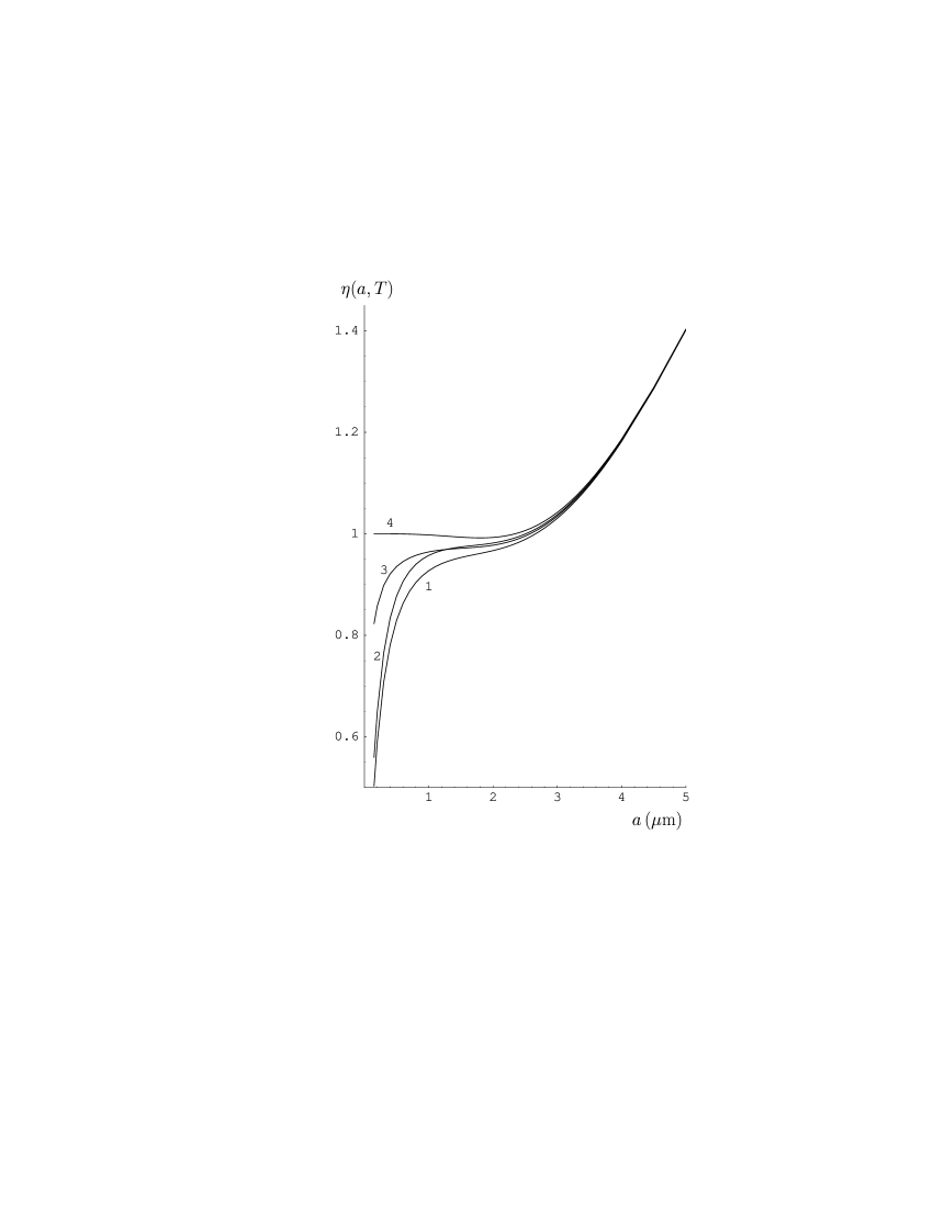
In Fig. 1 the values of the correction factor to the Casimir-Polder energy [see Eq. (15)] are presented for the atom He∗ near an Au wall [recall that the Casimir-Polder free energy is obtained as a product in accordance with Eq. (28)]. The curve 1 in Fig. 1 was computed by Eq. (29) at separations m and by Eq. (39) at separations m (for Au the plasma wavelength nm). Thus curve 1 represents our result for the correction factor accounting for the finite conductivity of the metal, the dynamic polarizability of the atom, and nonzero temperature.
For comparison, in Fig. 1 the other results for are plotted omitting various of the above factors. Curve 2 is obtained using Eqs. (29) and (39) as in curve 1, but with . Thus curve 2 represents an ideal metal wall with account of the dynamic polarizability of the atom and nonzero temperature. Curve 3 is also computed by Eqs. (29) and (39) but with all parameters thereby taking into account the nonideality of the metal and nonzero temperature but disregarding the dependence of the atomic polarizability on frequency. Finally, curve 4 is computed with Eqs. (29) and (39) but with both and . Curve 4 represents the case of an ideal metal at nonzero temperature and an atom described by the static polarizability. All curves 1–4 can be compared with a horizontal straight line (not shown) representing the case of an atom described by its static polarizability near a wall made of an ideal metal at zero temperature.
As is seen from Fig. 1, at short separations the effect of the finite conductivity of the wall metal in the case of an atom described by the static polarizability (compare the curves 3 and 4) is much greater than for an atom described by its dynamic polarizability (compare the curves 1 and 2). In particular, for a real atom near an Au wall the finite conductivity corrections are much less than for two metal plates. It is known 19 that for two parallel plates the use of the plasma model instead of the optical tabulated data leads to error up to 2%. In our case, however, the use of the plasma model dielectric function (19) leads to less than 1% error in the values of the Casimir-Polder free energy and force compared to the use of obtained by the optical tabulated data for the complex index of refraction. One can conclude also that at short separations the proper account of the atomic dynamic polarizability is more important than the proper account of the finite conductivity. This becomes clear if one compares curves 2 and 3 with curve 4. At intermediate separations of about 1 to m the atomic dynamic polarizability and the finite conductivity of the metal play qualitatively equal roles. As increases the dynamic polarizability become negligible and the free-energy is determined by only . Ultimately at separations m the high temperature asymptotic expression (31) for the ideal metal becomes applicable.
Overall, from Fig. 1 one can conclude that at the shortest separations considered here the corrections to the Casimir-Polder interaction due to different relevant factors can be as large as 35% and should be taken into account in comparison of measurement data with theory. At intermediate separations of about 1 to m the corrections may be of the order 5–7%, which is also rather significant.
Now we consider the computational results for the Casimir-Polder force. In Fig. 2 the values of the force correction factor versus separation are plotted for the He∗ atom near a Au wall [the force can be found from in accordance with Eq. (32), where was defined in Eq. (18)]. The correction factor was computed using Eq. (33) at separations m and using Eq. (41) at separations m. Curves 1–4 in Fig. 2 are numbered analogously to those in Fig. 1. Curve 1 takes into account all corrections to the Casimir-Polder force, i.e., the finite conductivity of the metal, the atomic dynamic polarizability, and nonzero temperature. Curve 2 was computed with (ideal metal), curve 3 with (atom with a frequency independent polarizability), and curve 4 with both .
The curves in Fig. 2 demonstrate qualitatively the same characteristic features as were already discussed with respect to Fig. 1. In particular, at short separations the effect of the finite conductivity is suppressed if the dynamic polarizability is taken into account (compare curves 3 and 4 with curves 1 and 2.) Accounting for the dynamic polarizability proves to be more important at small separations than does accounting for the finite conductivity (this becomes clear if one compares curves 2 and 3 with curve 1). At intermediate separations both effects lead to approximately equal contributions. At m the high temperature asymptote, given by Eq. (34) for the ideal metal, becomes applicable (at m the nonideality of a metal and frequency dependence of the polarizability of an atom are already negligible).
From Fig. 2 it is seen that the correction factors play a stronger role in the case of the force than for the free energy. For example, at the shortest separation considered here the overall correction factor is 57%. At intermediate separations of about 1 to m the correction factor for the force is 5–9%.
Let us now determine the accuracy of the obtained asymptotic expressions for the Casimir-Polder free energy [Eqs. (29) and (39)] and force [Eqs. (33) and (41)] and check that they smoothly join at approximately 1 to m. For this purpose we perform computations of the free energy and force for several different atoms using the asymptotic expressions and compare them with the result of numerical computations by the Lifshitz formulas (12) and (17). In doing so we will also check the accuracy of the single oscillator model for the dynamic polarizability, given by Eq. (43), by performing the test computations using accurate data for the atomic dynamic polarizability.
In Table I the computational results for the correction factor to the Casimir-Polder free energy at K are presented as functions of the separation distance listed in the first column. In column 2 the values of for a He∗ atom near an Au wall are computed numerically using the Lifshitz formula (12), dielectric permittivity (19) and the highly accurate non-relativistic atomic polarizability for the He∗ atom 36 . The dependence of the normalized dynamic atomic polarizability of He∗, , on frequency is shown by the curve 1 in Fig. 3 36 . The data of Fig. 3 have a relative error of about . It is interesting to compare them with the values given by the single oscillator model (43) (if plotted together as in Fig. 3 both sets of data would appear to coincide). The largest difference is expected at the shortest separation considered, i.e., at nm. Here the characteristic frequency is equal to . Numerical data of Fig. 3 show that at the differences in the relative polarizability between the single oscillator model and exact values are less than 1%. At higher frequencies these differences increase and have the value 28% at (the highest Matsubara frequency giving some minor contribution to the Casimir-Polder interaction). At a separation nm and for the highest contributing Matsubara frequency the single oscillator model leads to about 20% error.
Columns 3, 4, and 5 contain the values of for the He∗ atom near an Au wall computed, respectively, by the use of the Lifshitz formula (12), the asymptotic expression (29), and the asymptotic expression (39). To obtain the results of the second column, Eqs. (19) and (43) were substituted directly into the Lifshitz formula (12). Columns 6, 7, and 8 contain the analogous computational results for the Na atom, and columns 9, 10, and 11 for the Cs atom. The effective frequencies [see the explanations after Eq. (43)] for Na and Cs were found be equal to rad/s for Na and rad/s for Cs. For this purpose the equation and the data of Refs. 37 ; 37a for and were used.
As is seen from Table I (columns 2 and 3), the single oscillator model leads to practically the same results for the correction factor as the exact relative atomic polarizability. At the shortest separation nm, where the difference between the two computations is maximal, it is equal to only 0.14% of the result. This difference quickly decreases with increasing separation. Because of this, one can conclude that the Casimir-Polder free energy can be reliably computed by the use of the single oscillator model.
Now let us compare columns 2 and 3 of Table I with columns 3 and 4 representing the results obtained by the above asymptotic expressions. It is seen that the results of column 4 [asymptotic expression (29)] practically coincide with the data of columns 2 and 3 at large separations, and the results of column 5 [asymptotic expression (39)] coincide up to a fraction of percent with the same data at short separations. In the intermediate region of m both asymptotic expessions join smoothly deviating from results of columns 2 and 3 by about 0.4%.
Similar conclusions can be made from columns 6–8 (for Na) and columns 9–11 (for Cs). The single difference is that for Na the smooth joining of both asymptotic expressions take place at m, where the asymptotic values of the free energy deviate from the data of column 6 by about 0.2%. For Cs the asymptotic expressions for small and large separations join smoothly at m. At this separation they deviate from the numerical results of column 9 by approximately 0.3%.
It is notable that for the atoms of Na and Cs the single oscillator model for the dynamic polarizability is even more exact than for the atom of He∗. To illustrate this, in Fig. 3 the accurate normalized atomic dynamic polarizability of the Na atom is presented (curve 2) using the data of Ref. 37b . Here the differences with the dynamic polarizability given by the single oscillator model are much less than for the atom of He∗. At the shortest separation nm and at the highest Matsubara frequency contributing into the Casimir-Polder free energy there is only 4% difference in the values of the exact and approximate relative polarizability. This does not lead to any noticeable change in the value of the correction factor . For Cs, its effective frequency is less than for Na but greater than for He∗. Thus there is only a 0.1% difference in the value of the correction factor occuring for Cs at the shortest separation nm. At larger separations the single oscillator model leads to exactly the same results for the Casimir-Polder free energy as the exact dynamic polarizability.
Now we compare the results of the asymptotic and numerical calculations of the Casimir-Polder force acting between different atoms and an Au wall. These results are presented in Table II in the form of correction factor [see Eqs. (32) and (41)]. Table II is organized similarly to Table I. Column 1 contains the values of separations, in column 2 the numerical computations of are presented for He∗ from the exact formula (26) with the dielectric permittivity (19) and accurate dynamic polarizability (curve 1 of Fig. 3). In columns 3, 4, and 5 the values of for He∗ are calculated by Eq. (26) with the single oscillator model, Eq. (33) at large separations and Eq. (41) at short separations, respectively. Columns 6–8 and 9–11, respectively, contain similar data for the atoms Na and Cs, as are given in columns 3–5 for He∗.
From columns 2 and 3 it is seen that use of the the single oscillator model to calculate the force is a bit less exact than it was in the case of the free energy calculation. But even here the maximal error of introduced by the single oscillator model at a separation nm is only 0.3%. The comparison of columns 2 or 3 with columns 4 and 5 shows that the smooth joining of the two asymptotes occurs at m. At this separation each asymptote deviates from the numerical result by less than 0.5%. For the atoms Na and Cs, respectively, the smooth joining of the asymptotes for the force correction factor takes place at m and m.
Both Tables I and II demonstrate that the single oscillator model and the corresponding asymptotic formulas for large and short separations can be reliably used to calculate the Casimir-Polder free energy and force for different atoms near a metal wall with a precision to better than 1%.
V Conclusions and discussion
In the above we have performed both analytical and numerical calculations of the Casimir-Polder interaction of different atoms and a gold cavity wall with account of real experimental conditions such as the nonideality of a metal wall, dynamic polarizability of the atom, and nonzero temperature. These calculations demonstrate significant deviations from the classical Casimir-Polder results (up to 35% for the free energy and up to 57% for the force in the case of He∗ atom near an Au wall at the shortest separation considered in the paper where the thermal corrections are still negligible). We conclude that the proper account of real conditions is necessary for interpretation of measurement data in precision cavity QED experiments.
The simple and transparent derivation of the Lifshitz formula for the free energy of atom-wall interaction was performed at nonzero temperature of a wall in terms of the reflection coefficients starting from the usual Lifshitz formula for two semispaces. In the limiting case of an ideal metal and an atom described by the static polarizability the classical Casimir-Polder result was reproduced.
The combined account of different corrections to the Casimir-Polder energy and force indicate that at short separations (larger than the plasma wavelength of a wall metal) the corrections due to the dynamic polarizability play a much more important role than do the corrections due to the nonideality of a wall metal. Moreover, it was found that the dynamic polarizability of an atom leads to the suppression of the finite conductivity corrections in comparison to the static polarizability case.
On the basis of the Lifshitz formula for the atom-wall interaction, two asymptotic expressions for the Casimir-Polder free energy and force were obtained, one of which is applicable at large separations and the other one at short separations. The asymptotic formula for large separations takes exact account of nonzero temperature and is presented in the form of double perturbation theory in powers of two small parameters, the relative penetration depth of electromagnetic oscillations into a wall metal () and the relative characteristic frequency of an atom (). The asymptotic formula for short separations was derived at zero temperature. It takes into account exactly the atomic dynamic polarizability and treats perturbatively, in powers of a small parameter , the nonideality of the metal. In the region of intermediate separations both asymptotic formulas join smoothly. It is notable that the single oscillator model for the atomic dynamic polarizability (although it may deviate up to 30% from the exact data at some contributing Matsubara frequencies with large numbers) leads to practically exact results for the Casimir-Polder free energy and force. We therefore conclude that the analytical expressions obtained for the Casimir-Polder interaction can be combined with the single oscillator model for the dynamic polarizability preserving the final accuracy of approximately 1%.
The important question for further discussion would the obtained results be applicable in the case when the cavity wall is at a temperature but the atom belongs to the Bose-Einstein condensate with a temperature . According to our expectations, the above results would indeed apply to a Bose-Einstein condensate and a wall. We believe this is so because the Bose-Einstein condensate would have very low relative kinetic energy among the atoms (they can be described as ultracold atoms, but this is not the temperature that interests us), however the atoms would still be subject to the fluctuating fields present in the spatial vacuum separating the Bose-Einstein condensate and the cavity wall, characterized by the temperature .
One more important correction factor which was not discussed above is the wall roughness. As was shown in Ref. 38 , the roughness contribution to the Casimir-Polder force between an atom and a wall can be rather significant leading to qualitative physical effects. The role of roughness can be taken into account in combination with the other corrections by the method of the geometrical averaging 14 ; 19 ; 33 . The diffraction-type and other nonadditive contributions to the roughness corrections can be estimated along the lines of Refs. 33 ; 39 . However, the investigation of the role of roughness should be adapted to some definite experiment and be based on the atomic force 14 and (or) scanning electron 40 microscope images of the wall surface profiles.
Acknowledgments
G.L.K. and V.M.M. are grateful to P. W. Milonni for stimulating discussions. This work was supported by the National Science Foundation through a grant for the Institute for Theoretical Atomic, Molecular and Optical Physics at Harvard University and Smithsonian Astrophysical Observatory. G.L.K. and V.M.M. were partially supported by Finep (Brazil). V.M.M. was partially supported by CAPES (Brazil).
References
- (1) J. Mahanty and B. W. Ninham, Dispersion Forces (Academic Press, London, 1976).
- (2) F. Shimizu, Phys. Rev. Lett. 86, 987 (2001).
- (3) V. Druzhinina and M. DeKieviet, Phys. Rev. Lett. 91, 193202 (2003).
- (4) Y. Lin, I. Teper, C. Chin, and V. Vuletić, Phys. Rev. Lett. 92, 050404 (2004).
- (5) R. E. Grisenti, W. Schollkopf, J. P. Toennies, G. C. Hegerfeldt, and T. Kohler, Phys. Rev. Lett. 83, 1755 (1999).
- (6) J. D. Perreault, A. D. Cronin, and T. A. Savas, e-print physics/0312123.
- (7) J. E. Lennard-Jones, Trans. Faraday Soc. 28, 333 (1932).
- (8) H. B. G. Casimir and D. Polder, Phys. Rev. 73, 360 (1948).
- (9) A. Shih, D. Raskin, and P. Kusch, Phys. Rev. A 9, 652 (1974).
- (10) A. Shih, Phys. Rev. A 9, 1507 (1974).
- (11) A. Shih and V. A. Parsegian, Phys. Rev. A 12, 835 (1975).
- (12) E. Zaremba and W. Kohn, Phys. Rev. A 13, 2270 (1976).
- (13) G. Vidali and M. W. Cole, Surf. Sci. 110, 10 (1981).
- (14) A. Anderson, S. Haroche, E. A. Hinds, W. Jhe, and D. Meschede, Phys. Rev. A 37, 3594 (1988).
- (15) V. Sandoghdar, C. I. Sukenik, and E. A. Hinds, Phys. Rev. Lett. 68, 3432 (1992).
- (16) M. Oria, M. Chrevrollier, D. Bloch, M. Fichet, and M. Ducloy, Europhys. Lett. 14, 527 (1991).
- (17) C. I. Sukenik, M. G. Boshier, D. Cho, V. Sandoghdar, and E. A. Hinds, Phys. Rev. Lett. 70, 560 (1993).
- (18) S. K. Lamoreaux, Phys. Rev. Lett. 78, 5 (1997).
- (19) U. Mohideen and A. Roy, Phys. Rev. Lett. 81, 4549 (1998); G. L. Klimchitskaya, A. Roy, U. Mohideen, and V. M. Mostepanenko, Phys. Rev. A 60, 3487 (1999).
- (20) B. W. Harris, F. Chen, and U. Mohideen, Phys. Rev. A 62, 052109 (2000).
- (21) G. Bressi, G. Carugno, R. Onofrio, and G. Ruoso, Phys. Rev. Lett. 88, 041804 (2002).
- (22) F. Chen, U. Mohideen, G. L. Klimchitskaya, and V. M. Mostepanenko, Phys. Rev. Lett. 88, 101801 (2002); Phys. Rev. A 66, 032113 (2002).
- (23) R. S. Decca, D. López, E. Fischbach, and D. E. Krause, Phys. Rev. Lett. 91, 050402 (2003); R. S. Decca, E. Fischbach, G. L. Klimchitskaya, D. E. Krause, D. López, and V. M. Mostepanenko, Phys. Rev. D 68, 116003 (2003).
- (24) M. Bordag, U. Mohideen, and V. M. Mostepanenko, Phys. Rep. 353, 1 (2001).
- (25) P. Treutlein, P. Hommelhoff, T. Steinmetz, T. W. Hänsch, and J. Reichel, Phys. Rev. Lett. 92, 203005 (2004).
- (26) A. E. Leanhardt, Y. Shin, A. P. Chikkatur, D. Kielpinski, W. Ketterle, and D. E. Pritchard, Phys. Rev. Lett. 90, 100404 (2003).
- (27) D. M. Harber, J. M. McGuirk, J. M. Obrecht, and E. A. Cornell, J. Low Temp. Phys. 133, 229 (2003).
- (28) E. M. Lifshitz, Zh. Eksp. Teor. Fiz. 29, 94 (1956) [Sov. Phys. JETP 2, 73 (1956)].
- (29) I. E. Dzyaloshinskii, E. M. Lifshitz, and L. P. Pitaevskii, Usp. Fiz. Nauk 73, 381 (1961) [Sov. Phys. Usp. (USA) 4, 153 (1961)].
- (30) E. M. Lifshitz and L. P. Pitaevskii, Statistical Physics, Part. II (Pergamon Press, Oxford, 1980).
- (31) F. Zhou and L. Spruch, Phys. Rev. A 52, 297 (1995).
- (32) J. Schwinger, L. L. DeRaad, Jr., and K. A. Milton, Ann. Phys. (N.Y.) 115, 1 (1978).
- (33) P. W. Milonni, The Quantum Vacuum (Academic Press, San Diego, 1994).
- (34) M. Boström and B. E. Sernelius, Phys. Rev. A 61, 052703 (2000).
- (35) B. Geyer, G. L. Klimchitskaya, and V. M. Mostepanenko, Phys. Rev. A 67, 062102 (2003).
- (36) H. B. G. Casimir, Proc. K. Ned. Akad. Wet. 51, 793 (1948).
- (37) M. Bordag, e-print hep-th/0403222.
- (38) G. Barton, J. Phys. B 7, 2134 (1974); G. Barton, in: Special Issue: Casimir Forces, eds. J. F. Babb, P. W. Milonni, and L. Spruch. Comm. Mod. Phys. 1, 301 (2000).
- (39) M. Boström and B. E. Sernelius, Phys. Rev. Lett. 84, 4757 (2000).
- (40) J. S. Høye, I. Brevik, J. B. Aarseth, and K. A. Milton, Phys. Rev. E 67, 056116 (2003).
- (41) V. B. Bezerra, G. L. Klimchitskaya, and V. M. Mostepanenko, Phys. Rev. A 66, 062112 (2002).
- (42) V. B. Bezerra, G. L. Klimchitskaya, V. M. Mostepanenko, and C. Romero, Phys. Rev. A 69, 022119 (2004).
- (43) F. Chen, G. L. Klimchitskaya, U. Mohideen, and V. M. Mostepanenko, Phys. Rev. A 69, 022117 (2004).
- (44) I. S. Gradshtein and I. M. Ryzhik, Table of Integrals, Series and Products (Academic Press, New York, 1980).
- (45) R. Brühl, P. Fouquet, R. E. Grisenti, J. P. Toennies, G. C. Hegerfeldt, T. Köhler, M. Stoll, and C. Walter, Europhys. Lett. 59, 357 (2002).
- (46) Z.-C. Yan and J. F. Babb, Phys. Rev. A 58 1247 (1998).
- (47) A. Derevianko, W. R. Johnson, M. S. Safronova, and J. F. Babb, Phys. Rev. Lett. 82, 3589 (1999).
- (48) A. Derevianko and S. G. Porsev, Phys. Rev. A 65, 053403 (2002).
- (49) P. Kharchenko, J. F. Babb, and A. Dalgarno, Phys. Rev. A 55, 3566 (1997).
- (50) V. B. Bezerra, G. L. Klimchitskaya, and C. Romero, Phys. Rev. A 61, 022115 (2000).
- (51) T. Emig, A. Hanke, R. Golestanian, and M. Kardar, Phys. Rev. Lett. 87, 260402 (2001); Phys. Rev. A 67, 022114 (2003).
- (52) J. Esteve, C. Aussibal, T. Schumm, C. Figl, D. Mailly, I. Bouchoule, Ch. Westbrook, and A. Aspect, e-print physics/0403020.


| Metastable He∗ near Au wall | Na near Au wall | Cs near Au wall | ||||||||
|---|---|---|---|---|---|---|---|---|---|---|
| (m) | (a) | (b) | (c) | (d) | (b) | (c) | (d) | (b) | (c) | (d) |
| 0.15 | 0.5039 | 0.5032 | 0.5050 | 0.6415 | 0.6452 | 0.5705 | 0.5731 | |||
| 0.2 | 0.5899 | 0.5900 | 0.5912 | 0.7194 | 0.7217 | 0.6551 | 0.6567 | |||
| 0.3 | 0.7070 | 0.7077 | 0.7083 | 0.8124 | 0.8134 | 0.7630 | 0.7637 | |||
| 0.4 | 0.7801 | 0.7810 | 0.7814 | 0.8635 | 0.8640 | 0.8259 | 0.8264 | |||
| 0.5 | 0.8285 | 0.8294 | 0.8298 | 0.8946 | 0.8950 | 0.8657 | 0.8661 | |||
| 0.6 | 0.8620 | 0.8627 | 0.8632 | 0.9149 | 0.9154 | 0.8922 | 0.8928 | |||
| 0.7 | 0.8859 | 0.8865 | 0.8872 | 0.9289 | 0.9235 | 0.9297 | 0.9108 | 0.9116 | ||
| 0.8 | 0.9035 | 0.9040 | 0.9051 | 0.9390 | 0.9354 | 0.9401 | 0.9243 | 0.9254 | ||
| 0.9 | 0.9167 | 0.9172 | 0.9187 | 0.9464 | 0.9440 | 0.9480 | 0.9342 | 0.9283 | 0.9358 | |
| 1.0 | 0.9269 | 0.9272 | 0.9294 | 0.9520 | 0.9502 | 0.9541 | 0.9418 | 0.9375 | 0.9439 | |
| 1.1 | 0.9347 | 0.9350 | 0.9281 | 0.9379 | 0.9562 | 0.9549 | 0.9590 | 0.9475 | 0.9444 | 0.9504 |
| 1.2 | 0.9409 | 0.9411 | 0.9360 | 0.9448 | 0.9594 | 0.9584 | 0.9520 | 0.9496 | 0.9556 | |
| 1.3 | 0.9458 | 0.9460 | 0.9420 | 0.9504 | 0.9619 | 0.9612 | 0.9555 | 0.9537 | 0.9599 | |
| 1.4 | 0.9498 | 0.9499 | 0.9468 | 0.9552 | 0.9640 | 0.9633 | 0.9583 | 0.9569 | ||
| 1.5 | 0.9531 | 0.9532 | 0.9508 | 0.9592 | 0.9656 | 0.9651 | 0.9606 | 0.9596 | ||
| 2.0 | 0.9668 | 0.9669 | 0.9659 | 0.9741 | 0.9739 | 0.9712 | 0.9708 | |||
| 2.5 | 0.9889 | 0.9889 | 0.9885 | 0.9935 | 0.9934 | 0.9917 | 0.9914 | |||
| 3.0 | 1.031 | 1.031 | 1.030 | 1.034 | 1.033 | 1.032 | 1.032 | |||
| 3.5 | 1.096 | 1.096 | 1.095 | 1.097 | 1.097 | 1.097 | 1.097 | |||
| 4.0 | 1.182 | 1.182 | 1.182 | 1.183 | 1.183 | 1.183 | 1.183 | |||
| 4.5 | 1.286 | 1.286 | 1.285 | 1.286 | 1.286 | 1.286 | 1.286 | |||
| 5.0 | 1.402 | 1.402 | 1.402 | 1.402 | 1.402 | 1.402 | 1.402 | |||
| 6.0 | 1.656 | 1.656 | 1.656 | 1.656 | 1.656 | 1.656 | 1.656 | |||
| 7.0 | 1.924 | 1.924 | 1.924 | 1.924 | 1.924 | 1.924 | 1.924 | |||
| 8.0 | 2.196 | 2.196 | 2.196 | 2.196 | 2.196 | 2.196 | 2.196 | |||
| Metastable He∗ near Au wall | Na near Au wall | Cs near Au wall | ||||||||
|---|---|---|---|---|---|---|---|---|---|---|
| (m) | (a) | (b) | (c) | (d) | (b) | (c) | (d) | (b) | (c) | (d) |
| 0.15 | 0.4298 | 0.4284 | 0.4309 | 0.5707 | 0.5762 | 0.4959 | 0.4995 | |||
| 0.2 | 0.5151 | 0.5146 | 0.5163 | 0.6553 | 0.6586 | 0.5835 | 0.5858 | |||
| 0.3 | 0.6388 | 0.6394 | 0.6402 | 0.7625 | 0.7640 | 0.7028 | 0.7039 | |||
| 0.4 | 0.7214 | 0.7224 | 0.7229 | 0.8246 | 0.8254 | 0.7769 | 0.7775 | |||
| 0.5 | 0.7787 | 0.7798 | 0.7811 | 0.8637 | 0.8641 | 0.8257 | 0.8260 | |||
| 0.6 | 0.8198 | 0.8208 | 0.8211 | 0.8899 | 0.8902 | 0.8593 | 0.8596 | |||
| 0.7 | 0.8500 | 0.8511 | 0.8513 | 0.9083 | 0.9085 | 0.8834 | 0.8837 | |||
| 0.8 | 0.8729 | 0.8739 | 0.8741 | 0.9218 | 0.9221 | 0.9013 | 0.9016 | |||
| 0.9 | 0.8905 | 0.8914 | 0.8918 | 0.9320 | 0.9276 | 0.9324 | 0.9149 | 0.9152 | ||
| 1.0 | 0.9056 | 0.9052 | 0.9057 | 0.9399 | 0.9368 | 0.9405 | 0.9254 | 0.9259 | ||
| 1.1 | 0.9155 | 0.9161 | 0.9036 | 0.9170 | 0.9461 | 0.9438 | 0.9469 | 0.9336 | 0.9280 | 0.9345 |
| 1.2 | 0.9244 | 0.9249 | 0.9154 | 0.9261 | 0.9509 | 0.9492 | 0.9522 | 0.9402 | 0.9359 | 0.9414 |
| 1.3 | 0.9312 | 0.9318 | 0.9246 | 0.9337 | 0.9547 | 0.9533 | 0.9565 | 0.9453 | 0.9420 | 0.9471 |
| 1.4 | 0.9371 | 0.9374 | 0.9317 | 0.9400 | 0.9576 | 0.9565 | 0.9494 | 0.9468 | 0.9520 | |
| 1.5 | 0.9416 | 0.9418 | 0.9373 | 0.9454 | 0.9598 | 0.9589 | 0.9525 | 0.9504 | 0.9560 | |
| 2.0 | 0.9515 | 0.9516 | 0.9498 | 0.9623 | 0.9620 | 0.9580 | 0.9572 | |||
| 2.5 | 0.9505 | 0.9506 | 0.9498 | 0.9577 | 0.9575 | 0.9549 | 0.9545 | |||
| 3.0 | 0.9507 | 0.9507 | 0.9503 | 0.9556 | 0.9555 | 0.9537 | 0.9534 | |||
| 3.5 | 0.9620 | 0.9620 | 0.9617 | 0.9653 | 0.9652 | 0.9640 | 0.9639 | |||
| 4.0 | 0.9902 | 0.9902 | 0.9900 | 0.9925 | 0.9924 | 0.9916 | 0.9915 | |||
| 4.5 | 1.037 | 1.037 | 1.037 | 1.038 | 1.038 | 1.038 | 1.038 | |||
| 5.0 | 1.100 | 1.100 | 1.100 | 1.101 | 1.101 | 1.100 | 1.100 | |||
| 6.0 | 1.261 | 1.261 | 1.261 | 1.262 | 1.262 | 1.262 | 1.262 | |||
| 7.0 | 1.450 | 1.450 | 1.450 | 1.450 | 1.450 | 1.450 | 1.450 | |||
| 8.0 | 1.649 | 1.649 | 1.649 | 1.649 | 1.649 | 1.649 | 1.649 | |||