PROBABILITIES FROM ENTANGLEMENT, BORN’S RULE $p_{k}=|\psi_{k}|^{2}$ FROM ENVARIANCE

Abstract

I show how probabilities arise in quantum physics by exploring implications of environment - assisted invariance or envariance, a recently discovered symmetry exhibited by entangled quantum systems. Envariance of perfectly entangled “Bell-like” states can be used to rigorously justify complete ignorance of the observer about the outcome of any measurement on either of the members of the entangled pair. For more general states, envariance leads to Born’s rule, $p_{k}\propto|\psi_{k}|^{2}$ for the outcomes associated with Schmidt states. Probabilities derived in this manner are an objective reflection of the underlying state of the system – they represent experimentally verifiable symmetries, and not just a subjective “state of knowledge” of the observer. Envariance - based approach is compared with and found superior to pre-quantum definitions of probability including the standard definition based on the ‘principle of indifference’ due to Laplace, and the relative frequency approach advocated by von Mises. Implications of envariance for the interpretation of quantum theory go beyond the derivation of Born’s rule: Envariance is enough to establish dynamical independence of preferred branches of the evolving state vector of the composite system, and, thus, to arrive at the environment - induced superselection (einselection) of pointer states, that was usually derived by an appeal to decoherence. Envariant origin of Born’s rule for probabilities sheds a new light on the relation between ignorance (and hence, information) and the nature of quantum states.

I Introduction

The aim of this paper is to derive Born’s rule [1] and to identify and analyse origins of probability and randomness in physics. The key idea we shall employ is environment - assisted invariance (or envariance) [2-4], a recently discovered quantum symmetry of entangled systems. Envariance allows one to use purity (perfect knowledge) of a joint state of an entangled pair to characterize unknown states of either of its components and to quantify missing information about either member of the pair.

The setting of our discussion is essentially the same as in the study of decoherence and einselection [3,5-9]. However, the tools we shall employ differ. Thus, as in decoherence, the system of interest ${\cal S}$ is “open” and can be entangled with its environment ${\cal E}$. We shall, however, refrain from using “trace” and “reduced density matrix”. Their physical significance is based on Born’s rule [10,11]. Therefore, to avoid circularity, we shall focus on pure global quantum states which yield – as a consequence of envariance – mixed states of their components. Successful derivation of Born’s rule will in turn justify the usual interpretation of these formal tools while shedding a new light on the foundations of quantum theory and its relation with information.

The nature of “missing information” and the origin of probabilities in quantum physics are two related themes, closely tied to its interpretation. We will be therefore forced to examine, in light of envariance, the structure of the whole interpretational edifice. These fragments that depend on decoherence and einselection will have to be rebuilt without the standard tools such as trace and reduced density matrices. Once Born’s rule is “off limits”, the problem becomes not just to derive probabilities, and, thus, to crown the already largely finished structure with $p_{k}=|\psi_{k}|^{2}$ as a final touch. Rather, the task is to deconstruct the interpretational edifice standing on an incomplete, shaky foundation, and to re-build it using these elements of the old plan that are still viable, but on a new, solid and deep foundations and, to a large extent, from new, more basic building blocks. We start in the next section with the proof that leads from envariance to Born’s rule. This will provide an overview of key ideas and their implications.

The original presentations of envariance [2-4] as well as most of this paper assume that quantum theory is universally valid. They rely only on unitary quantum evolutions and thus can be (as is decoherence) conveniently explored in the relative state framework [12] (although their results are independent of interpretation). One may equally well – as was emphasized by Howard Barnum [13] – analyze envariance in a ‘Copenhagen setting’ that includes the collapse postulate. Section II bypasses the discussion of quantum measurements and is in that sense most explicitly interpretation - neutral study of the consequences of envariance.

The goal of this paper is to understand the nature of probabilities and to derive Born’s rule in bare quantum theory. Thus, only unitary evolutions are allowed. The effective collapse (usually modeled with the help decoherence, which is in effect “off limits” here) is all one can hope for. The ground for the solution of the problem of the emergence of probabilities in this setting is explored and prepared in Section III. We start by comparing envariant definition of probability with the approaches used in classical physics, and go on to examine quantum measurements. “Symptoms of the classical” (such as the preferred basis) that are taken for granted in justifying the need for probabilities and are usually derived with the help of the trace operation and reduced density matrices are pointed out. As these tools depend on Born’s rule, their physical implications such as decoherence and einselection have to be re-examined and often re-derived if we are to avoid circularity, and we set the stage for this in Section III.

Preferred pointer states are such a necessary pre-condition for the emergence of the classical. Pointer states define what information is missing – what are the potential measurement outcomes, providing ‘menu’ of the alternative future events the observer may be ignorant of. Hence, they are indispensable in defining probabilities. Pointer states are recovered in Section IV without decoherence – without relying on tools that implicitly invoke Born’s rule: We show how environment - induced superselection can be understood through direct appeal to the nature of the quantum correlations, and, in particular, to envariance. This pivotal result – in a sense ‘einselection without decoherence’ – allows us to avoid any circularity in the discussion. It is based on the analysis of correlations between the system and the apparatus pointer (or the memory of the observer) in presence of the environment. It allows one to define future events – “buds” of the dynamically independent branches that can be assigned probabilities.

Section V discusses probabilities from the “personal point of view” of an observer described by quantum theory. Probabilities arise when the outcome of a measurement that is about to be performed cannot be predicted with certainty from the available data, even though observer knows all that can be known – the initial pure state of the system.

Relative frequencies of outcomes are considered in the light of envariance in section VI, shedding a new light on the connection between envariance and the statistical implications of quantum states.

In course of the analysis we shall discover that none of the standard classical approaches to probability apply directly in quantum theory. In a sense, common statement of the goal – “recovering classical probabilities in the quantum setting” – may have been the key obstacle in making progress because it was not ambitious enough. To be sure, it was understood long ago that none of the traditional approaches to the definition of probability in the classical world were all that convincing: They were either too subjective (relying on the analysis of observers’ “state of mind”, his lack of knowledge about the actual state) or too artificial (requiring infinite ensembles).

Complementarity of quantum theory provides the ‘missing ingredient’ that allows us to define probabilities using objective properties of entangled quantum states: Observer can know completely a global pure state of a composite system. That global state will have objective symmetries: They can be experimentally verified and confirmed using transformations and measurements that yield outcomes with certainty (and, hence, that do not involve Born’s rule). These objective properties of the global state imply – as we shall see – probabilities for the states of local subsystems. Perfect information about the whole can be thus used to demonstrate and quantify ignorance about a part. Circularity of classical approaches (which assume ignorance – e.g., “equal likelihood” – to establish ignorance – probabilities) is avoided: Probabilities enter as an objective property of a state. They reflect perfect knowledge (rather than ignorance) of the observer. These and other interpretational issues are discussed in Section VII.

This paper can be read either in the order of presentation, or ‘like an onion’, starting from the outer layers (Sections II and VII, followed by III and IV, etc.)

II Probabilities from envariance

To derive Born’s rule we recognize that;

(o)

the Universe consists of systems;

(i)

a completely known (pure) state of system ${\cal S}$ can be represented by a normalized vector in its Hilbert space ${\cal H_{S}}$;

(ii)

a composite pure state of several systems is a vector in the tensor product of the constituent Hilbert spaces;

(iii)

states evolve in accord with the Schrödinger equation $i\hbar|\dot{\psi}\rangle=H|\psi\rangle$ where $H$ is hermitean.

In other words, we start with the usual assumptions of the ‘no collapse’ part of quantum mechanics. We have listed them here in a somewhat more ‘fine-grained’ manner than it is often seen, e.g. in Ref. [3].

II.1 Environment - assisted invariance

Envariance is a symmetry of composite quantum states: When a state $|\psi_{\cal SE}\rangle$ of a pair of systems ${\cal S,~{}E}$ can be transformed by $U_{\cal S}=u_{\cal S}\otimes{\bf 1}_{\cal E}$ acting solely on ${\cal S}$,

$$U_{\cal S}|\psi_{\cal SE}\rangle=(u_{\cal S}\otimes{\bf 1}_{\cal E})|\psi_{\cal SE}\rangle=|\eta_{\cal SE}\rangle\ ,$$

but the effect of $U_{\cal S}$ can be undone by acting solely on ${\cal E}$ with an appropriately chosen $U_{\cal E}={\bf 1}_{\cal S}\otimes u_{\cal E}$:

$$U_{\cal E}|\eta_{\cal SE}\rangle=({\bf 1}_{\cal S}\otimes u_{\cal E})|\eta_{\cal SE}\rangle=|\psi_{\cal SE}\rangle\ ,$$

then $|\psi_{\cal SE}\rangle$ is called envariant under $U_{\cal S}$.

In contrast to the usual symmetries (that describe situations when the action of some transformation has no effect on some object) envariance is an assisted symmetry: The global state is transformed by $U_{\cal S}$, but can be restored by acting on ${\cal E}$, some other subsystem of the Universe, physically distinct (e.g., spatially separated) from ${\cal S}$. We shall call the part of the global state that can be acted upon to affect such a restoration of the preexisting global state the environment ${\cal E}$. Hence, the environment - assisted invariance, or – for brevity – envariance. We shall soon see that there may be more than one such subsystem. In that case we shall use ${\cal E}$ to designate their union. Moreover, on occasion we shall consider manipulating or measuring ${\cal E}$. So the oft repeated (and largely unjustified; see Refs. [3,4,8,14,15]) phrase ‘inaccessible environment’ should not be taken for granted here.

Envariance of pure states is a purely quantum symmetry: Classical state of a composite system is given by Cartesian (rather than tensor) product of its constituents. So, to completely know the state of a composite classical system one must know the state of each of its parts. It follows that when one part of a classical composite system is affected by the analogue of $U_{\cal S}$, the “damage” cannot be undone – the state of the whole cannot be restored – by acting on some other part of the whole. Hence, pure classical states are never envariant.

Another way of stating this conclusion is to note that states of classical objects are ‘absolute’, while in quantum theory there are situations – entanglement – in which states are relative. That is, in classical physics one would need to ‘adjust’ the remainder of the universe to exhibit envariance, while in quantum physics it suffices to act on systems entangled with the system of interest. For instance, in a hypothetical classical universe containing two and only two objects, a boost applied to either object could be countered by simultaneously applying the same boost to the other: The only motion in such a two - object universe is relative. Therefore, simultaneous boosts would make the new state of that hypothetical universe indistingushable from (and, hence, identical to) the initial pre-boost state. This will not work in our Universe, as the center of mass of the two boosted objects will be now moving with respect to the rest of its matter content. (That is, unless we make the second object the rest of our Universe: this thought experiment brings to mind the famous ‘Newton’s bucket’ – i.e., Newton’s suspicion that the meniscus formed by water rotating in a bucket would disappear if the rest of the Universe was forced to co-rotate.)

To give an example of envariance, consider Schmidt decomposition of $\psi_{\cal SE}$;

$$|\psi_{\cal SE}\rangle=\sum_{k=1}^{N}a_{k}|s_{k}\rangle|\varepsilon_{k}\rangle\ .$$

Above, by definition of Schmidt decomposition, $\{|s_{k}\rangle\}$ and $\{|\varepsilon_{k}\rangle\}$ are orthonormal and $a_{k}$ are complex. Any pure bipartite state can be written this way. A whole class of envariant transformations can be identified for such pure entangled quantum states:

Lemma 1. Any unitary transformation with Schmidt eigenstates $\{|s_{k}\rangle\}$;

$$u_{\cal S}=\sum_{k=1}^{N}\exp(i\phi_{k})|s_{k}\rangle\langle s_{k}|\ ,$$

is envariant.

Proof: Indeed, any unitary with Schmidt eigenstates can be undone by a ‘countertransformation’:

$$u_{\cal E}=\sum_{k=1}^{N}\exp(-i\phi_{k}+2\pi l_{k})|\varepsilon_{k}\rangle\langle\varepsilon_{k}|$$

where $l_{k}$ are arbitrary integers. QED.

Remark: The environment used to undo $u_{\cal S}$ need not be uniquely defined: For example, $u_{\cal S}$ acting on a GHZ-like state:

$$|\psi_{{\cal SEE}^{\prime}}\rangle=\sum_{k=1}^{N}a_{k}|s_{k}\rangle|\varepsilon_{k}\rangle|\varepsilon_{k}^{\prime}\rangle$$

can be envariantly undone by acting either on ${\cal E}$ or on ${\cal E}^{\prime}$, or by acting on both parts of the joint environment.

It is perhaps useful to point out that one can use $\psi_{\cal SEE^{\prime}}$ to obtain reduced density matrix:

$$\rho_{\cal SE}=\sum_{k}|a_{k}|^{2}|s_{k}\rangle\langle s_{k}|\otimes|\varepsilon_{k}\rangle\langle\varepsilon_{k}|$$

This means that even when the correlated state of ${\cal S}$ and ${\cal E}$ is mixed and of this form, one can in principle imagine that there is an underlying pure state. States of the above form can arise in measurements or as a consequence of decoherence. The discussion can be thus re-phrased in terms of pure states in all cases of interest. The assumption of suitable pure global state entails no loss of generality.

At first sight, envariance may not seem to be all that significant, since it is possible to show that it can affect only phases:

Lemma 2. All envariant unitary transformations have eigenstates that coincide with the Schmidt expansion of $|\psi_{\cal SE}\rangle$, i.e., have the form of Eq. (3a).

Proof is by contradiction: Suppose there is an envariant unitary $\tilde{u}_{\cal S}$ that cannot be made co-diagonal with Schmidt basis of $\psi_{\cal SE}$, Eq. (2). It will then inevitably transform Schmidt states of ${\cal S}$:

$$\tilde{u}_{\cal S}\otimes{\bf 1}_{\cal E}|\psi_{\cal SE}\rangle=\sum_{k=1}^{N}a_{k}(\tilde{u}_{\cal S}|s_{k}\rangle)|\varepsilon_{k}\rangle=\sum_{k=1}^{N}a_{k}|\tilde{s}_{k}\rangle|\varepsilon_{k}\rangle=|\tilde{\eta}_{\cal SE}\rangle\ .$$

If $\tilde{u}_{\cal S}$ is envariant there must be $\tilde{u}_{\cal E}$ such that

$${\bf 1}_{\cal E}\otimes\tilde{u}_{\cal E}|\tilde{\eta}_{\cal SE}\rangle=\sum_{k=1}^{N}a_{k}|s_{k}\rangle|\varepsilon_{k}\rangle=|\psi_{\cal SE}\rangle\ .$$

But unitary transformations acting exclusively on ${\cal H_{E}}$ cannot change states in ${\cal H_{S}}$. So, the new set of Schmidt states $|\tilde{s}_{k}\rangle$ of $\tilde{\eta}_{\cal SE}$ cannot be undone (‘rotated back’) to $|s_{k}\rangle$ by any $\tilde{u}_{\cal E}$. It follows that – when Schmidt states are uniquely defined – there can be no envariant unitary transformation that acts on the environment and restores the global state to $\psi_{\cal SE}$ after Schmidt states of ${\cal S}$ were altered by $\tilde{u}_{\cal S}$. QED.

Corollary: Properties of global states are envariant iff they are a function of the phases of the Schmidt coefficients.

Phases are often regarded as inaccessible, and are even sometimes dismissed as unimportant (textbooks tend to speak of a ‘ray’ in the Hilbert space, thus defining a state modulo its phase). Indeed, Schmidt expansion is occasionally defined by absorbing phases in the states which means that all the non-zero coefficients end up real and positive (and hence all the phases are taken to be zero). This is a dangerous oversimplification. Phases matter – reader can verify that it is impossible to write all of the Bell states when all the relative phases are set to zero. Indeed, the aim of the rest of this paper is, in a sense, to carefully justify when and for what purpose phases can be disregarded, and to understand nature of the ignorance about the local state of the system as a consequence of the global nature of these phases.

II.2 State of a subsystem of a quantum system

Independence of the state of the system ${\cal S}$ from phases of the Schmidt coefficients will be our first important conclusion based on envariance. To establish it we list below three facts – additional assumptions that may be regarded as obvious. We state them here explicitly to clarify and extend the meaning of terms ‘(sub)system’ and ‘state’ we have already used in axioms (o) - (iii).

Fact 1:

Unitary transformations must act on the system to alter its state. (That is, when the evolution operator does not operate on the Hilbert space ${\cal H_{S}}$ of the system, i.e., when it has a form $...\otimes{\bf 1}_{\cal S}\otimes...$ the state of ${\cal S}$ remains the same.)

Fact 2:

The state of the system ${\cal S}$ is all that is needed (and all that is available) to predict measurement outcomes, including their probabilities.

Fact 3:

The state of a larger composite system that includes ${\cal S}$ as a subsystem is all that is needed (and all that is available) to determine the state of the system ${\cal S}$.

We have already implicitly appealed to fact 1 earlier, e.g. in the proof of Lemma 2. Note that the above facts are interpretation - neutral and that states (e.g., ‘the state of ${\cal S}$’) they refer to need not be pure.

With the help of the facts can now establish:

Theorem 1. For an entangled global state of the system and the environment all measurable properties of ${\cal S}$ – including probabilities of various outcomes – cannot depend on the phases of Schmidt coefficients: The state of ${\cal S}$ has to be completely determined by the set of pairs $\{|\alpha_{k}|,~{}|s_{k}\rangle\}$.

Proof: Envariant transformation $u_{\cal S}$ could affect the state of ${\cal S}$. However, by definition of envariance the effect of $u_{\cal S}$ can be undone by a countertransformation of the form ${\bf 1}_{\cal S}\otimes u_{\cal E}$ which – by fact 1 – cannot alter the state of ${\cal S}$. As ${\cal SE}$ is returned to the initial state, it follows from fact 3 that the state of ${\cal S}$ must have been also restored. But (by fact 1) it could not have been effected by the countertransformation. So it must have been left unchanged by the envariant $u_{\cal S}$ in the first place. It follows (from the above and (fact 2) that measurable properties of ${\cal S}$ are unaffected by envariant transformations. But, by Lemma 1 & 2, envariant transformations can alter phases and only phases of Schmidt coefficients. Therefore, any measurable property of ${\cal S}$ implied by its state must indeed be completely determined by the set of pairs $\{|\alpha_{k}|,~{}|s_{k}\rangle\}$. QED.

Remark: Information content of the list $\{|\alpha_{k}|,~{}|s_{k}\rangle\}$ that describes the state of ${\cal S}$ is the same as the information content of the reduced density matrix. We do not know yet, however, what are the probabilities of various outcome states $|s_{k}\rangle$.

Thus, envariance of Schmidt phases proves that only absolute values of Schmidt coefficients can influence measurement outcomes. Yet, the dismissive attitude towards phases we have reported above is incorrect. This is best illustrated on an example: Changing phases between the Hadamard states;

$$|\pm\rangle=(|s_{1}\rangle\pm|s_{2}\rangle)/\sqrt{2}$$

can change the state of the system from $|s_{1}\rangle$ to $|s_{2}\rangle$. More generally;

Lemma 3. Iff the Schmidt decomposition of Eq. (2) has coefficients that have the same absolute value – that is, the state is even:

$$|\bar{\psi}_{\cal SE}\rangle\propto\sum_{k=1}^{N}e^{i\phi_{k}}|s_{k}\rangle|\varepsilon_{k}\rangle\ ,$$

it is also envariant under a swap:

$$u_{\cal S}(1\rightleftharpoons 2)=e^{i\phi_{12}}|s_{1}\rangle\langle s_{2}|+h.c.$$

Proof: By Lemma 1, swap is envariant – it can be generated by $u_{\cal S}$ diagonal in Hadamard basis of the two states (which is also Schmidt when their coefficients differ only by a phase). Swaps can be seen to be envariant also more directly: When $a_{1}=|a|e^{i\phi_{1}},\ a_{2}=|a|e^{i\phi_{2}}$, every swap can be undone by the corresponding counterswap:

$$u_{\cal E}(1\rightleftharpoons 2)=e^{-i(\phi_{12}+\phi_{1}-\phi_{2}+2\pi l_{12})}|\varepsilon_{1}\rangle\langle\varepsilon_{2}|+h.c.$$

This proves envariance of swaps for equal values of the coefficients of the swapped states. Converse follows from Lemma 1 & 2: Envariant transformations can affect only phases of Schmidt coefficients, so the global state cannot be restored after the swap when their absolute values differ. QED.

Remark: When ${\cal SE}$ is in an even state $|\bar{\psi}_{\cal SE}\rangle$ (that is therefore envariant under swaps) exchange $|s_{1}\rangle\rightleftharpoons|s_{2}\rangle$ does not affect the state of ${\cal S}$ – its consequences cannot be detected by any measurement of ${\cal S}$ alone.

Lemma 3 we have just established is the cornerstone of our approach. We now know that when the global state of ${\cal SE}$ is even (i.e., with equal absolute values of its Schmidt coefficients), then a swap (which predictably takes known $|s_{k}\rangle$ into $|s_{l}\rangle$) does not alter the state of ${\cal S}$ at all.

Envariantly swappable state of the system defines perfect ignorance. We emphasize the direction of this implication: The state of ${\cal S}$ is provably completely unknown not because of the subjective ignorance of the oberver. Rather, it is unknown as a consequence of complementarity: the state of ${\cal SE}$ is after all perfectly known. Moreover, it can be objectively known to many observers. All of them will agree that their perfect global knowledge implies complete local ignorance. Therefore, probabilities are objective properties of this state.

Symmetries of the state of ${\cal SE}$ imply ignorance of the observer about the outcomes of his future measurements on ${\cal S}$. This emergence of objective probabilities is purely quantum. Objective probabilities are incompatible with classical setting (where there is an unknown but definite preexisting state). In the quantum setting, objective nature of probabilities arises as a consequence of the entanglement, e.g., with the environment.

II.3 Born’s rule from envariance

So far, we have avoided refering to probabilities. Apart from brief mention in fact 2 and immediately above we have not discussed how do they relate to quantum measurements. This will have to wait for when we consider quantum measurements, records and observers from an envariant point of view. But it turns out that one can derive the rule connecting probabilities with entangled state vectors such as $|\psi_{\cal SE}\rangle$ of Eq. (2) from relatively modest assumptions about their properties. The next key step in this direction is:

Theorem 2. Probabilities of Schmidt states of ${\cal S}$ that appear in $|\psi_{\cal SE}\rangle$ with coefficients that have same absolute value are equal.

There are several inequivalent ways to establish Theorem 2. Indeed, the reader may feel that it was already established: Remark that followed Lemma 3 plus a rudimentary symmetry arguments suffice to do just that. However, for completeness, we now spell out some of these arguments in more detail. Both Barnum [13] and Schlosshauer and Fine [16] have discussed some of the related issues. Reporting some of their conclusions (and anticipating some of ours) it appears that envariance plus a variety of small subsets of natural assumptions suffice to arrive at the thesis of Theorem 2.

II.3.1 Envariance under complete swaps

We start with the first version of the proof:

(a)

When operations that swap any two orthonormal states leave the state of ${\cal S}$ unchanged, probabilities of the outcomes associated with these states are equal.

Proof (a) is immediate. When the entangled state of ${\cal SE}$ has equal values of the Schmidt coefficients, e.g. $|\bar{\psi}_{\cal SE}\rangle\propto\sum_{k=1}^{N}e^{i\phi_{k}}|s_{k}\rangle|\varepsilon_{k}\rangle$, local state of ${\cal S}$ will be indeed unaffected by the swaps (by Theorem 1 and Lemma 3 above). Consequently, with the assumption (a), thesis of Theorem 2 follows. QED.

The above argument is close in the spirit to Laplace’s “principle of indifference” [17]. We prove that swapping possible outcome states – shuffling cards – “makes no difference”. However, in contrast to Laplace we show ‘objective indifference’ of the physical state of the system in question rather than observers subjective indifference based on his state of knowledge.

Note that in absence of entanglement (and, hence envariance) swap generally changes the underlying state of the system also when coefficients of states corresponding to various potential outcomes have the same absolute values. For example, pure states $|\alpha\rangle\propto|1\rangle+|2\rangle-|3\rangle+|4\rangle$ and $|\beta\rangle\propto|1\rangle+|3\rangle-|2\rangle+|4\rangle$ are orthogonal even though they have the same absolute values of the coefficients and differ only by a swap. Thus, without entanglement with the environment (i.e., in absence of Lemma 1 & 2 and, hence, Theorem 1 that allows one to ignore phases of Schmidt coefficients) assumption (a) would be tantamount to assertion that phases of the coefficients are unimportant in specifying the state. For isolated systems this is obviously wrong, in blatant conflict with the quantum principle of superposition!

In absence of envariance the key to our argument – assertion that the state of ${\cal S}$ is left unchanged by a swap – is simply wrong. This is easily seen by considering ensemble of identical pure states (such as $|\alpha\rangle$). Through measurements, observer can find out the state of systems in that ensemble (e.g., $|\alpha\rangle$ or $|\beta\rangle$). By contrast, if this ensemble becomes first entangled with the environment in such a way that $|1\rangle\dots|4\rangle$ are Schmidt, an observer with access to ${\cal S}$ only would conclude that the state of the system is a perfect mixture, and would not be able to tell if the pre-decoherence state was $|\alpha\rangle$ or $|\beta\rangle$.

II.3.2 Envariance under partial swaps and dynamics

The second strategy we shall use to prove Theorem 2 relies on a somewhat different ‘dynamical’ definition of indifference. We note that when we have some information about the state, we should be able to “detect motion” (possibly using an ensemble of such states) – to observe changes caused by the dynamical evolution. This intuition is captured by our assumption:

(b)

When the state of ${\cal S}$ is left unchanged by all conceivable unitary transformations acting on a subspace $\tilde{\cal H}_{\cal S}$ of ${\cal H_{S}}$, then probabilities of all the outcomes of any exhaustive measurement corresponding to any orthocomplete basis that spans that subspace of $\tilde{\cal H}_{\cal S}$ are the same.

To proceed we first establish that when complete swaps, Eq. (6a), between a subset of states of some orthonormal basis that spans $\tilde{\cal H}_{\cal S}$ leave the state of ${\cal S}$ unchanged, then so do partial swaps on the same subspace:

Lemma 4: Partial swaps defined by pairwise exchange of any two orthonormal basis sets $\{|s_{k}\rangle\}$ and $\{|\tilde{s}_{l}\rangle\}$ that span even subspace ${\bar{\cal H}_{\cal S}}$ of ${\cal H_{S}}$ which admits full swaps, Eq. (6a) – are also envariant.

Proof: Partial swap can be expressed as a unitary;

$$\tilde{u}_{\cal S}(\{\tilde{s}_{k}\}\rightleftharpoons\{s_{k}\})=\sum_{|s_{k}\rangle\in\bar{\cal H_{S}}}|\tilde{s}_{k}\rangle\langle s_{k}|\ .$$

This is the obvious generalization of the simple swap of Eq. (6a). $\tilde{u}_{\cal S}(\{\tilde{s}_{k}\}\rightleftharpoons\{s_{k}\})$ can be undone by the corresponding partial counterswap of the Schmidt partners of the swapped pairs of states. It follows from Lemma 3 that $\bar{\psi}_{\cal SE}$ – a state envariant under complete swaps – must have a form:

$$|\bar{\psi}_{\cal SE}\rangle\propto\sum_{k=1}^{K}e^{i\phi_{k}}|s_{k}\rangle|\varepsilon_{k}\rangle$$

where $K=Dim(\bar{\cal H_{S}})$. Basis $\{|\tilde{s}_{l}\rangle\}$ spans the same subspace $\bar{\cal H}_{\cal S}$. Therefore,

$$|\bar{\psi}_{\cal SE}\rangle\propto\sum_{l=1}^{K}|\tilde{s}_{l}\rangle(\sum_{k=1}^{K}e^{i\phi_{k}}\langle\tilde{s}_{l}|s_{k}\rangle|\varepsilon_{k}\rangle)=\sum_{l=1}^{K}|\tilde{s}_{l}\rangle|\tilde{\varepsilon}_{l}\rangle\ .$$

Given that $\{|\varepsilon_{k}\rangle\}$ are Schmidt, it is straightforward to verify that $\{|\tilde{\varepsilon}_{l}\rangle\}$ are orthonormal, and, therefore, the expansion on RHS above is also Schmidt. Consequently;

$$\tilde{u}_{\cal E}(\{\tilde{\varepsilon}_{k}\}\rightleftharpoons\{\varepsilon_{k}\})=\sum_{\varepsilon_{k}\in\bar{\cal H_{E}}}|\tilde{\varepsilon}_{k}\rangle\langle\varepsilon_{k}|\ ,$$

the desired partial counterswap exists. This establishes envariance under partial swaps. QED.

Corollary: When complete swaps are envariant in the subspace $\bar{\cal H_{S}}\in{\cal H_{S}}$, so are all the unitary transformations on $\bar{\cal H_{S}}$. Indeed, the set of all partial swaps is the same as the set of all unitary transformations on the subspace $\bar{\cal H_{S}}$.

We can now give the second proof of Theorem 2:

Proof (b): Equality of probabilities under envariant swaps follows immediately from the above Corollary and assumption (b). QED.

Using Lemma 4 and its Corollary, we can identify mathematical objects that represent even states in ${\cal H_{S}}$: Only a uniform distribution of pure states over $\bar{\cal H}_{\cal S}$ is invariant under all unitaries. The alternative representation that is more familiar is the (reduced) density matrix. It has to be proportional to the identity operator:

$$\rho_{\cal S}\propto{\bf 1}_{\cal S}\ ,$$

to be invariant under all unitaries.

So envariance, the no collapse axioms (o)-(iii), plus the three facts imply that our abstract state (whose role is defined by fact 2) leads to the distribution uniform in the Haar measure or, equivalently to the reduced density matrix $\propto{\bf 1}_{\cal S}$ within $\bar{\cal H}_{\cal S}$. Note that these conclusions follow from Lemma 4, which does not employ assumption (b). The form of the mathematical object representing envariantly swappable state of ${\cal S}$ follows directly from the symmteries of the underlying entangled composite state of ${\cal SE}$. In particular, we have in a sense obtained the reduced density matrix in the special case without the usual arguments [10,11], i.e., without relying on Born’s rule. Moreover, assumption (b) is needed only when we want to interpret that reduced density matrix in terms of probabilities.

Assumption (b) can also be regarded as a quantum counterpart of Laplace’s principle of indifference [17]. Now there are however even more obvious differences between the quantum situation and shuffling cards than these we have already mentioned in the discussion of proof (a). Classical deck cannot be shuffled into a superposition of the original cards. This can obviously happen to a ‘quantum deck’: In quantum physics we can consider arbitrary unitary transformations (and not just discrete swaps). This consequence of the nature of quantum evolutions can be traced all the way to the principle of superposition (and, hence, to phases!).

The other distinction between the quantum and classical principle of indifference we have already noted is even more striking: In classical physics it was the “state of knowledge” of the observer – his description of the system – that may (or may not) have been altered by the evolution – the underlying physical state was always affected when shuffling / evolution was non-trivial. In quantum theory there is no distinction between the epistemic ‘state of knowledge’ role of the state and its objective (‘ontic’) role. In this sense quantum states are ‘epiontic’ [3].

Probabilities are – in any case – an objective reflection of symmetries of such states: They follow from quantum complementarity between the global and local observables. They can be defined and quantified using envariance, an experimentally verifiable property of entangled quantum states.

II.3.3 Equal probabilities from perfect ${\cal SE}$ correlations

Both of the proofs above start with the assumption that under certain conditions probabilities of a subset of states of the system are equal, and then establish the thesis by showing that this assumption is implied by envariance under swaps – both are in that sense Laplacean. The third proof also starts with an assumption of equality of probabilities, but now we consider relation between the probabilities of the Schmidt states of ${\cal S}$ and ${\cal E}$. This approach (Barnum [13], see also discussion in Ref. [16]) recognizes that pairs of Schmidt states ($|s_{k}\rangle|\varepsilon_{k}\rangle$ in Eq. (2)) are perfectly correlated, which implies that they have the same probabilities. Thus, one can prove equality of probabilities of envariantly swappable Schmidt states directly from envariance by relying on perfect correlations between Schmidt states of ${\cal S}$ and ${\cal E}$.

To demonstrate this equality we consider a subspace of ${\cal H_{S}}$ spanned by Schmidt states $|s_{k}\rangle$ and $|s_{l}\rangle$, so that the corresponding fragment of $\psi_{\cal SE}$ is given by:

$$|\psi_{\cal SE}\rangle=\dots+a_{k}|s_{k}\rangle|\varepsilon_{k}\rangle+a_{l}|s_{l}\rangle|\varepsilon_{l}\rangle+\dots$$

We assume that:

(c)

In the Schmidt decomposition partners are perfectly correlated, i.e., detection of $|s_{k}\rangle$ implies that in a subsequent measurement of Schmidt observable (i.e., observable with Schmidt eigenstates) on ${\cal E}$ will certainly obtain $|\varepsilon_{k}\rangle$ (this ‘partner state’ will be recorded with certainty, e.g., with probability 1).

Proof (c): From assumption (c) we immediately have that

$$p_{\cal S}(s_{k(l)})=p_{\cal E}(\varepsilon_{k(l)})\ .$$

Consider now a swap $s_{k}\rightleftharpoons s_{l}$. It leads from $\psi_{\cal SE}$, Eq. (2), to:

$$|\eta_{\widetilde{\cal S}{\cal E}}\rangle=\dots+a_{k}|s_{l}\rangle|\varepsilon_{k}\rangle+a_{l}|s_{k}\rangle|\varepsilon_{l}\rangle+\dots$$

Now, using again (c) we get;

$$p_{\widetilde{\cal S}}(s_{k(l)})=p_{\cal E}(\varepsilon_{l(k)})=p_{\cal S}(s_{l(k)})\ .$$

In effect, this establishes the ‘pedantic assumption’ of [2,3] using envariance and perfect correlation assumption (c): Probabilities get exchanged when the states are swapped. So we could go back to the proof of Ref. [2] with a somewhat different motivation. But we can also continue, and consider a counterswap in ${\cal E}$ that yields:

$$|\vartheta_{\widetilde{\cal S}\widetilde{\cal E}}\rangle=\dots+a_{k}|s_{l}\rangle|\varepsilon_{l}\rangle+a_{l}|s_{k}\rangle|\varepsilon_{k}\rangle+\dots$$

We now consider the case when $|a_{k}|=|a_{l}|=a$. Counterswap restores such an even state;

$$|\bar{\vartheta}_{\widetilde{\cal S}\widetilde{\cal E}}\rangle=\dots+a|s_{l}\rangle|\varepsilon_{l}\rangle+a|s_{k}\rangle|\varepsilon_{k}\rangle+\dots=|\bar{\psi}_{\cal SE}\rangle\ .$$

By facts 2 and 3 the overall state as well as the state of ${\cal S}$ must have been restored to the original. Therefore $p_{\widetilde{\cal S}}(s_{l(k)})=p_{\cal S}(s_{l(k)})$. Together with $p_{\widetilde{\cal S}}(s_{l(k)})=p_{\cal S}(s_{k(l)})$ established before this yields:

$$p_{\cal S}(s_{l(k)})=p_{\cal S}(s_{k(l)})$$

when the relevant Schmidt coefficients have equal absolute values. QED.

We have now established that in an entangled state in which all of the coefficients have the same absolute value so that every state $|s_{k}\rangle$ can be envariantly swapped with every other state $|s_{l}\rangle$, $|\bar{\psi}_{\cal SE}\rangle\propto\sum_{k=1}^{N}e^{i\phi_{k}}|s_{k}\rangle|\varepsilon_{k}\rangle$, all the possible orthonormal outcome states have the same probability. Let us also assume that states that do not appear in the above superposition (i.e., appear with Schmidt coefficient zero) have zero probability. (We shall motivate this rather natural assumption later in the paper.) Given the customary normalisation of probabilities we get for even (‘Bell-like’) states:

Corollary For states with equal absolute values of Schmidt coefficients;

$$p_{k}=p(s_{k})=1/N\ \ \ \forall k\ .$$

Moreover, probability of any subset of $n$ mutually exclusive events is additive. Hence:

$$p_{k_{1}\vee k_{2}\vee\dots\vee k_{n}}=p(s_{k_{1}}\vee s_{k_{2}}\vee\dots\vee s_{k_{n}})=n/N\ .$$

Above, we have assumed that orthogonal states correspond to mutually exclusive events. We shall motivate also this (very natural) assumption of the additivity of probabilities further in discussion of quantum measurements in Section V (thus going beyond the starting point of e.g. Gleason[30]). Here we only note that while additivity of probabilities looks innocent, in the quantum case (where the principle of superposition entitles one to add complex amplitudes) it should not be taken for granted. In the end, we shall conclude that additivity of probabilities is tied to envariance, which yields phases (and, hence, quantum superposition principle) irrelevant for Schmidt states of the subsystems of the entagled whole.

We also note that the probability entered our discussion in a manner that bypasses circularity: We have simply identified certainty with the probability of 1 (see e.g. assumption (c) above). This provides us with the normalization, while the symmetries revealed by envariance determine probabilities in the case when there is no certainty.

II.4 Born’s rule: the case of unequal coefficients

To complete derivation of Born’s rule consider the case when the absolute values of the coefficients $a_{k}$ in the Schmidt decomposition are proportional to $\sqrt{m_{k}}$, where $m_{k}$ are natural numbers.

$$|\psi_{\cal SE}\rangle\propto\sum_{k=1}^{N}\sqrt{m_{k}}e^{i\phi_{k}}|s_{k}\rangle|\varepsilon_{k}\rangle\ .$$

We now introduce a counterweight / counter ${\cal C}$. It can be thought of either as a subsystem extracted from the environment ${\cal E}$, or as an ancilla that becomes correlated with ${\cal E}$ so that the combined state is:

$$|\psi_{\cal SEC}\rangle\propto\sum_{k=1}^{N}\sqrt{m_{k}}e^{i\phi_{k}}|s_{k}\rangle|\varepsilon_{k}\rangle|C_{k}\rangle\$$

where $\{|C_{k}\rangle\}$ are orthonormal. Moreover, we assume that $|C_{k}\rangle$ are associated with subspaces of ${\cal H_{C}}$ of sufficient dimensionality so that the ‘fine-graining’ represented by:

$$|C_{k}\rangle=\sum_{j_{k}=\mu_{k-1}+1}^{\mu_{k}}|c_{j_{k}}\rangle/\sqrt{m_{k}}$$

is possible. Above, $\mu_{k}=\mu_{k-1}+m_{k}$, and $\mu_{0}=0$.

We also utilize a c-shift, a c-not - like gate[3] that correlates states of ${\cal E}$ with the fine-grained states of ${\cal C}$:

$$|c_{j_{k}}\rangle|\varepsilon_{k}\rangle\longrightarrow|c_{j_{k}}\rangle|e_{j_{k}}\rangle\ ,$$

where $|e_{j_{k}}\rangle$ are orthonormal states of $\cal E$ that correlate with the individual states of the counter $\cal C$ (e.g., causing decoherence). We have now arrived at the state vector that represents a perfectly entangled (equal coefficient, or ‘even’) state of the composite system consisting of ${\cal SC}$ and ${\cal E}$:

$$|\Psi_{\cal SEC}\rangle\propto\sum_{j_{k}=1}^{M}e^{i\phi_{j_{k}}}|s_{k(j_{k})},c_{j_{k}}\rangle|e_{j_{k}}\rangle\ .$$

Above, $M=\sum_{k=1}^{N}m_{k}=\mu_{N}$, and $k=k(j)$ is the obvious “staircase” function, i.e. when $\mu_{k-1}<j\leq\mu_{k}$, then $k(j)=k$.

The state $\Psi_{\cal SEC}$ is envariant under swaps of joint Schmidt states $|s_{k(j_{k})},c_{j_{k}}\rangle$ of ${\cal SC}$. Hence, by Eq. (7a):

$$p_{j_{k}}\equiv p(c_{j_{k}})\equiv p(|s_{k(j_{k})},c_{j_{k}}\rangle)=1/M$$

Moreover, Eq. (7b) implies that if we were to enquire about the probability of the state of ${\cal S}$ alone, the answer must be given by:

$$p_{k}\ \equiv\sum_{j_{k}=\mu_{k-1}+1}^{\mu_{k}}p(|s_{k(j_{k})},c_{j_{k}}\rangle)=m_{k}/M\ =\ |a_{k}|^{2}\ .$$

This is Born’s rule. The extension to the case where $|a_{k}|^{2}$ are incommensurate is straightforward by continuity as rational numbers are dense among reals.

III Envariance, Ignorance, and Chance

We have now presented a fairly complete discussion of envariance, and we have derived Born’s rule. The aim of the rest of this paper is to consider some of the other implications of envariance for our quantum Universe. This section serves the role of the intermission after the first act of a play. The basic plot is already in place. We can now take a few moments to speculate on how it will develop. In particular, we shall compare definition of probabilities based on envariance with the pre-quantum discussions of this concept. We shall also set the stage for the investigation of the implications of envariance for the interpretation of quantum theory. This includes (but is not limited to) the issue of the ‘decoherence-free’ derivation of the preferred pointer basis.

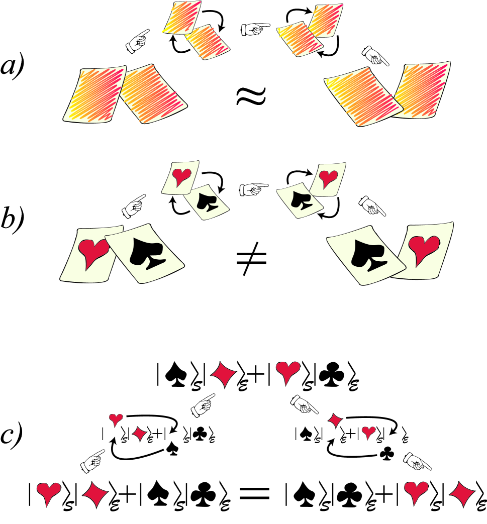
Figure 1: Envariance is related to the ‘principle of indifference’ (or the ‘principle of equal likelihood’) used by Laplace [17] to define subjective probabilities. However in quantum physics envariance leads to probabilities based on an objective symmetries of the underlying physical state of the system. The principle of indifference is illustrated in Fig. 1a. An observer (or a card player) who knows one of the two cards is $\spadesuit$ but does not see their faces does not care – is indifferent – when cards get swapped (even when he needs $\spadesuit$ to win). When the probability of a favorable outcome is the same before and after the swap then the states are equivalent (“$\approx$”) from his point of view. This leads to subjective probabilities given by the ratio of the number of favorable outcomes to the total; $p_{\spadesuit}={1\over 2}$. Laplace’s approach based on observers ignorance and not on the actual physical state is often regarded as the sole justification of Bayesian view. It is controversial. In particular, it does not reflect the actual ‘physical’ state of the system: As seen in Fig. 1b, states before and after the swap are not equivalent, “$\neq$”. Fig 1c shows how quantum theory leads to probabilities based on the physical state when the system of interest when ${\cal S}$ is entangled with ‘the environment’ ${\cal E}$. Such entanglement would occur as a result of decoherence. When ${\cal S}$ and ${\cal E}$ are maximally entangled, the swap on ${\cal S}$ has no effect on its state. This is clear, since its effect can be undone without acting on ${\cal S}$ – by a ‘counterswap’ that involves only ${\cal E}$. The final states are simply the same, so the probability of the swapped states of ${\cal S}$ must also be the same! Envariance can be used to prove (see Theorem 2) that for such ‘even’ entangled states that have the same absolute values of the coefficients (which makes them envariantly swappable), probabilities of mutually exclusive alternatives (orthonormal Schmidt states) are equal. Generalization of to the case of unequal coefficients is straightforward and establishes Born’s rule $p_{k}=|\psi_{k}|^{2}$.

III.1 Envariance and the ‘principle of indifference’

The idea that invariance under swaps implies ignorance and hence probabilities is old, and goes back at least to Laplace [17]. We illustrate it in Fig. 1a. The appeal to invariance under swaps leads to a definition that is known as ‘standard’ (or, sometimes, ‘classical’ – the adjective we reserve in this paper for its other obvious meaning). In classical physics standard definition has to be applied with apologies, as it refers to observers’ subjective lack of knowledge about the system, rather than to the objective properties of state of the system per se. That the observer (player) does not care about (is indifferent to) swapping of the cards in a shuffled deck is the consequence of the fact that he does not know their ‘face values’. It is a subjective reason – not reflected in the objective symmetries of the actual state of the deck (see Fig. 1b). To recognise this, it is said that certain possible states are, in his subjective judgement, ‘equally likely’.

As always in physics, subjectivity is a source of trouble. In case of the above ‘principle of indifference’ this trouble is exacerbated by the fact that the objective classical state (e.g., of the deck of cards) is well defined and does not respect ‘symmetries of the state of mind’ of the observer.

Subjectivity was the principal reason this ‘standard definition of probabilities’ has fallen out of favor, and was largely replaced by the ‘relative frequency approach’ [18-20]. We shall not discuss it in detail as yet, but we remind the reader that in this approach probability of a certain event – i.e., a certain outcome – is given by its relative frequency in an infinite ensemble.

There are problems with this strategy as well. My discomfort with relative frequencies stems from the fact that infinite ensembles generally do not exist, and, hence, have to be imagined – i.e., must be subjectively extrapolated from finite sets of data. So, subjectivity cannot be convincingly exorcised in this manner.

I bring up relative frequencies here only to note that the strategy of using swaps to define equiprobable events would work also in this setting. When a swap (i.e., re-labeling all $s_{k}$ as $s_{l}$ – e.g, renaming “heads” as “tails” and vice versa) applied to an ensemble leaves all the relative frequencies of the swapped states unchanged, their probabilities must have been equal. In a sense, this observation may be regarded as an independent motivation of the assumption (a) above.

In quantum physics, exact symmetry of a composite state – envariance – can be used to demonstrate that the observer need not care about swapping, as envariant swapping provably cannot alter anything in his part of the bipartite system when $\psi_{\cal SE}$ is ‘even’ – that is, of the form given by Eq. (5). We illustrate it in Fig. 1c. As we have already seen, envariance makes ignorance and probabilities easier to define. The circularity of the ‘standard definition’ is easier to circumvent in the quantum setting. It is however important to understand what fixes this ‘menu of options’, and to find out when they can be regarded as effectively classical.

III.2 Quantum and classical ignorance

Motivating the need for probabilities using ignorance about a preexisting state is often regarded as synonymous with the ignorance interpretation. We have relied on a similar approach. However, for our purpose a narrowly classical definition of ignorance through an appeal to definite classical possibilities one of which actually exists independently of observer and can be discovered by his measurements without being perturbed is simply too restrictive: Observer can be ignorant of the outcome of his future measurement also when the system in question is quantum and when there are no fixed pre-existing alternatives. He can then choose between various non-commuting observables and sets of alternative ‘events’ defined by their complementary eigenstates. That choice of what to measure determines what is it observer is ignorant about – what sort of information his about-to-be-performed measurement will reveal.

Quantum definition of probabilities based on envariance is superior to the above mentioned classical approaches because it justifies ignorance objectively, without appealing to observers’ subjective ‘lack of knowledge’. Entangled quantum state of ${\cal SE}$ (or any pair of entangled systems) can be perfectly known to the observer beforehand. There can be multiple records of that state spread throughout the environment, making it ‘operationally objective’ – simultaneously accessible to many observers. They can use its objective global properties to demonstrate – employing real swaps one can carry out in the laboratory – that the outcomes of some of the measurements one can perform are provably swappable, and, hence, equiprobable. In this sense, observers can directly measure probabilities of various outcomes without having to find out first what these outcomes are.

Note that this can be accomplished without an appeal to an “ensemble”, “likelihood”, or any other surrogate for probability: All that is needed is a single system $\cal S$, as well as appropriate ${\cal E}$ and ${\cal C}$. The entangled states we have studied in the preceding section can be then created, and their symmetries can be verified through manipulations and measurements. Moreover, the measurements involved have outcomes that can be predicted with certainty. This is how the concept of probability enters our discussion. Observer is certain of the global state, and (using envariance) can count the number of envariantly swappable (and, hence, equiprobable) outcomes.

The aim of the observer is to use records of the outcomes of past measurements (his data) that in effect define the global state to predict future events – his future record of the measurement of the local system. Tools that can be legally employed in this task include observers knowledge of the ‘no collapse’ quantum physics, encapsulated in the opening paragraph of Section II, as well as the facts 1-3 of the preceding section. They do not include Born’s rule: Hence the trace operation, reduced density matrices, etc. are ‘off limits’ in our derivations (although when we succeed, embargo on their use will be lifted).

In the no-collapse settings, effective classicality of the memory can be justified through appeal to decoherence [3-8,15]. But here we cannot appeal to full-fledged decoherence, cannot rely on trace, etc. Is there still a way to recover enough of the ‘effectively classical’ to justify existence of classical records we took for granted in the preceding section?

III.3 Problems of ‘no collapse’ approaches

There were several attempts to make sense of probabilities in the ‘no collapse’ setting [21-25]. They have relied almost exclusively on relative frequencies (counting probabilities) [21-23]. The aim was to show that, in the limit of infinitely many measurements, only branches in which relative frequency definition would have given the answer for probabilities consistent with Born’s rule have a non-vanishing measure. However, that meant dismissing infinitely many (‘maverick’) branches where this is not the case, because their amplitude becomes negligible in the same infinite limit. All of these attempts have been shown to use circular arguments [25-29]: In effect, they were all forced to assume that relative weights of the branches are based on their amplitudes. That meant that another measure was introduced, without physical justification, in order to legitimize use of relative frequency measure based on counting.

By contrast, derivations of Born’s rule that assume ‘collapse’ either explicitly [30,32] or implicitly [31], that is by considering ab initio infinite ensembles of identical systems so that ‘branches’ with ‘wrong’ relative frequency of counts simply disappear as their amplitudes vanish in the infinite ensemble limit have been successful (although see [33] for a somewhat more critical assessment of Refs. [31,32]).

Indeed, Gleason’s theorem [30] is now an accepted and rightly famous part of quantum foundations. It is rigorous – it is after all a theorem about measures on Hilbert spaces. However, regarded as a result in physics it is deeply unsatisfying: it provides no insight into physical significance of quantum probabilities – it is not clear why the observer should assign probabilities in accord with the measure indicated by Gleason’s approach [22-29,31-34]. This has motivated various primarily frequentist approaches [22-29,,31,32,34]. However, as was already noted in the discussion of the relative frequency approach, appeal to infinite ensembles is highly suspect, especially when – as is the case here – the desired effect is achieved only when the size of ensemble $N=\infty$ [27-29,33].

In view of these difficulties, some have even expressed doubts as to whether there is any room for the concept of probability in the no-collapse setting [26-29]. This concern is on occasion traced all the way to the identity of the observer who could define and make use of probabilities in Many Worlds universe. Such criticism was often amplified by pointing out that, in the pre-decoherence versions of Everett - inspired interpretations, decomposition of the universal state vector is not unique (see e.g. comments in Ref. [27]) so it is not even clear what ‘events’ should such probabilities refer to. This difficulty was regarded by some as so severe that even staunch supporters of Everett considered adding an ad hoc rule to quantum theory to specify a preferred basis (see e.g. Ref. [35]) in clear violation of the spirit of the original relative state proposal [12].

Basis ambiguity was settled by einselection [3-9,14,15]. But standard tools of decoherence are ‘off limits’ here. And even if we were to accept decoherence - based resolution of basis ambiguity and used einselected pointer states to define branches, we would be still faced with at least one remaining aspect of the ‘identity crisis’: In course of a measurement the memory of the observer ‘branches out’ so that it appears to record (and, hence, critics conclude, observer should presumably perceive) all of the outcomes. If that were so, then there would be no room for distinct outcomes, choice, and hence, no need for probabilities.

Existential interpretation is based on einselection [3,8,15] and can settle also this aspect of the identity crisis. It follows physical state of the observer by tracking its evolution, also in course of measurements. Complete description of observers’ state includes physical state of his memory, which is updated as he acquires new records. So, what the observer knows is inseparable from what the observer is. Observer who has acquired new data does not lose his identity: He simply extends his records – his history. Identity of the observer as well as his ability to measure persist as long as such updates do not result in too drastic a change of that state (see Wallace [36] for a related point of view). For instance, Wigner’s friend would be able to continue to act as observer with reliable memory in each ‘outcome branch’, but the same cannot be said about the Schrödinger’s cat.

But the existential interpretation depends on decoherence. Threfore, we have to either disown it altogether while embarking on the derivation of Born’s rule, or re-establish its foundations without relying on trace and reduced density matrices to derive Born’s rule. Once we are successfull, we can then proceed to reconstruct all of the “standard lore” of decoherence, including all of its interpretational implications, on a firm and deep foundation – quantum symmetry of entangled states.

We note that when (at the risk of circularity we have detailed above) decoherence is assumed, Born’s rule can be readily derived using variety of approaches [8,24] including versions of both standard and frequentist points of view [8] as well as approaches based on decision theory [24,36] suggested by Deutsch and Wallace. I shall comment on these in Section VII.

IV Pointer states, records, and ‘events’

Probability is a tool observers employ in the absence of certainty to predict their future (including in particular future state of their own memory) using the already available data – present state of their memory. Sometimes these data can determine some of the future events uniquely. However, often predictions will be probabilistic – the observer may count on one of the potential outcomes, but will not know which one. Our task is to replace questions that uncertain outcomes of future measurement on the system with situations that allow for a certainty of prediction about the effect of some actions (swaps) on an enlarged system. In that sense we are reducing questions about probabilities in general to the straightforward case – to the questions that yield answers with certainty (i.e., with probability of 1). This special case makes the connection with probability in the situation when probability is known. It provides us with the overall normalization. Using this connection, we then infer probabilities of possible outcomes of measurements on ${\cal S}$ from the analogue of the Laplacean ‘ratio of favorable events to the total number of equiprobable events’, which we shall see in Section V is a good definition of quantum probabilities for events associated with effectively classical records kept in pointer states. In quantum physics this ratio can be determined using envariance and even verified experimentally prior to finding out what the event is. But we do need events. Hence, we need pointer states.

In classical physics it can be always assumed that a random event was pre-determined – i.e., that the to-be-discovered state existed objectively beforehand and was only revealed by the measurement. Indeed, such objective preexistence is often regarded as a pre-condition of the ‘ignorance interpretation’ of probabilities. In quantum physics, as John Archibald Wheeler put it paraphrasing Niels Bohr, “No phenomenon is a phenomenon untill it is a recorded phenomenon” [37]. Objective existence cannot be attributed to quantum states of isolated, individual systems. When the system is being monitored by the environment, one may approximate objective existence by selectively proliferating quantum information (this is the essence of quantum Darwinism). Operational definition of objectivity – one of the key symptoms of classicality – can be recovered using this idea, as selective proliferation leads to many copies of the information about the same ‘fittest’ observable.

Here we deal with individual quantum events – outcomes of future measurements on individual quantum systems, not carried out as yet. They need not (and, in general, do not) preexist even in the sense of quantum Darwinism – selective proliferation of information has not happened as yet. The observer will decide what observable he will measure (and, hence, what information will get proliferated, and become effectively classical). The menu of events should be determined by the observable he chooses to measure.

Objective pre-existence of events is not needed before the measurement. On the other hand, as noted above, we need some aspects of classicality to represent memory of the observer after the measurement. Objectivity would be best, but we can settle for less: The key ingredient is the existence of well-defined ‘events’ – record states that, following measurement, will reliably preserve correlation with the recorded state of the system in spite of the immersion of the memory in the environment. Pointer states [5-9] are called for, but we are not allowed to use decoherence.

There are at least three reasons why preferred states (that are stable in spite of the opennes of the system) are essential. The original reason for their introduction [5] was to assure that observers’ memory is effectively classical – einselection of preferred basis ascertains that his ‘hardware’ can keep records only in the pointer basis.

It follows that model observers will store and process information more or less like us (and more or less like a classical computer). For instance, human brain is a massivelly parallel, and as yet far from understood, but nevertheless classical information processing device. And classical records cannot exist (cannot be accessed) in superpositions.

A more pertinent reason to look for preferred states is the recognition that the information processing hardware of observers is open – immersed in the environment. Interaction with ${\cal E}$ is a fact of life. Unless we find in the memory Hilbert space ‘quiet corners’ that remain quiet in spite of this openness, reliable memory (and hence reliable information processing) will not be possible.

Last not least, the very idea of measuring makes sense only if measurement outcomes can be used for prediction. But most of the systems of interest are ‘open’ as well. Therefore, predictability can be hoped for only in special cases – for the einselected pointer states of systems that can remain correlated with the apparatus that has measured them [5,6,8].

Decoherence methods used to analyse consequences of such immersion in the environment employ reduced density matrices and trace [3-9,14,15]. They are based on Born’s rule. Once decoherence is assumed, Born’s rule can be readily derived [8], but this strategy courts circularity [3,38]. Obviously, if we temporarily renounce decoherence (so that we can attempt to derive $p_{k}=|\psi_{k}|^{2}$) we have to find some other way to either justify existence of pointer states and the einselection - based definition of branches in a decoherence - independent manner, or give up and conclude that while Born’s rule is consistent with decoherence, it cannot be established from more basic principles in a no-collapse setting. We shall show that, fortunately, preferred states do obtain more or less directly from envariance. That is, environment - induced superselection, and, hence, pointer basis and branches can be defined by analysing correlations between quantum systems, very much in the spirit of the original ‘pointer basis’ proposal [5], and without the danger of circularity that may have arisen from reliance on trace and reduced density matrices.

IV.1 Relative states and definite outcomes: Modeling the collapse

The essence of the ‘no collapse’ approach is its relative state nature – its focus on correlations. Once we identify possible record states of the memory, the correlation between them and the states of the relevant fragments of the Universe is all that matters: Observer will be ‘aware’ of what he knows, and all he knows is represented by his data. The key is, however to identify relative pointer states that are suitable as memory states.

We start our discussion with a confirmatory pre-measurement in which there is no need for the full-fledged ‘collapse’. Observer is presented with a system in a state $\varphi$, and told to measure observable that has $\varphi$ as one of its eigenstates. He need not know the outcome beforehand. Given a set of potential mutually exclusive outcomes $\{\dots,\varphi,\dots\}$ observer can devise an interaction that will – with certainty – lead to:

$$|A_{0}\rangle^{\otimes{\cal N}}|\varphi\rangle\ {\buildrel{\{\dots\varphi\dots\}}\over{\longrightarrow}}|A_{0}\rangle^{\otimes{\cal N}-1}|A_{\varphi}\rangle|\varphi\rangle\ .$$

Above, ‘ready to record’ memory cells are designated by $|A_{0}\rangle$, and the symbol above the arrow representing measurement indicates that the set of possible outcomes includes $\varphi$. This pre-measurement can be repeated many ($m$) times:

$$|A_{0}\rangle^{\otimes{\cal N}}|\varphi\rangle\ \ {\buildrel{\{\dots\varphi\dots\}}\over{\underbrace{\longrightarrow\dots\longrightarrow}_{m}}}\ \ |A_{0}\rangle^{\otimes{\cal N}-m}|A_{\varphi}\rangle^{\otimes m}|\varphi\rangle\ .$$

Each new outcome can be predicted by the observer from the first record providing that – as we assume here and below – there is no evolution between measurements and that the measured observable does not change.

In spite of the concerns we have reported before there is no threat to the identity of the observer. Moreover, in view of the recorded evidence, Eq. (11b), and his ability to predict future outcomes in this situation, observer may assert that the system is in the state $\varphi$. Indeed, if we did not assume that our observer is familiar with quantum physics, we could try and convince him that – in view of the evidence – the system must have been in the preexisting ‘objective state’ $\varphi$ already before the first measurement. This happens to be the case in our example, but the state of a single system is not ‘objective’ in the same absolute sense one may take for granted in the classical realm: Obviously, in quantum theory a long sequence of records after the measurement is no guarantee of the ‘objective preexistence’ of the observer - independent state before the measurement in the same sense as was the case in the classical realm.

When the observer subsequently decides to measure a different observable with the eigenstates $\{|s_{k}\rangle\}$ such that:

$$|\varphi\rangle=\sum_{k=1}^{N}\langle s_{k}|\varphi\rangle|s_{k}\rangle$$

the overall state viewed ‘from the outside’ will become:

$$|A_{0}\rangle^{\otimes{\cal N}-m}|A_{\varphi}\rangle^{\otimes m}|\varphi\rangle$$

$${\buildrel{\{|s_{k}\rangle\}}\over{\longrightarrow}}|A_{0}\rangle^{\otimes{\cal N}-m-1}|A_{\varphi}\rangle^{\otimes m}\sum_{k=1}^{N}\langle s_{k}|\varphi\rangle|A_{k}\rangle|s_{k}\rangle\ .$$

It is tempting to regard each sequence of records as a ‘branch’ of the above state vector. It certainly represents a possible state of the observer with the data concerning his ‘history’, including records of the state of the system. From his point of view, observer can therefore describe this ‘personal’ recorded history as follows: ‘As long as I was measuring observables with the eigenstate $\varphi$, the outcome was certain – it was always the same. After the first measurement, there was no surprise. In that operational sense the system was in the state $|\varphi\rangle$. When I switched to measuring $\{|s_{k}\rangle\}$, the outcome became (say) $|s_{17}\rangle$, and the system was in that state thereafter.’ This conclusion follows from his records:

$$\dots|A_{\varphi}\rangle^{\otimes m}|\varphi\rangle\ {{\buildrel{\{|s_{k}\rangle\}}\over{\longrightarrow}}}\dots|A_{\varphi}\rangle^{\otimes m}|A_{17}\rangle|s_{17}\rangle$$

$${{\buildrel{\{|s_{k}\rangle\}}\over{\underbrace{\longrightarrow\dots\longrightarrow}_{l-1}}}}\ \ \dots|A_{\varphi}\rangle^{\otimes m}|A_{17}\rangle^{\otimes l}|s_{17}\rangle\ .$$

There will be, of course, $N$ such branches, each of them labeled by a specific record (e.g., $\dots|A_{16}\rangle^{\otimes l},~{}|A_{17}\rangle^{\otimes l},~{}|A_{18}\rangle^{\otimes l}\dots$). But, especially when records are well - defined and stable, then there is again no threat to the identity of the observer. (Also note that in the equation above we have stopped counting the “still available” empty memory cells. In the tradition that dates back to Turing we shall assume, from now on, that observer has enough ‘blank memory’ to record whatever needs to be recorded.)

Now come the two key lessons of this section: To ‘first approximation’, from the point of view of the evidence (i.e., records in observer possession) there is no difference between the ‘classical collapse’ of many future possibilities into one present actuality he experiences after his first ‘confirmatory’ measurement, Eq. (11), and the ‘quantum collapse’, Eq. (13). Before the confirmatory measurement observer was told what observable he should measure, and he found out the state $\varphi$. A very similar thing happened when the observer switched to the different observable with the eigenstates $\{|s_{k}\rangle\}$: After the first measurement with an uncertain outcome a predictable sequence of confirmations followed.

In the ‘second approximation’, there is however an essential difference: In case of the classical collapse, Eq. (11), the observer had less of an idea about what to expect than in the case of genuine quantum measurement, Eq. (13). This is because now – in contrast to the “ersatz collapse” of Eq. (11) – observer knows all that can be known about the system he is measuring. Thus, in case of Eq. (11), observer did not know what to expect: He had no certifiably accurate information that would have allowed him to gauge what will happen. He could have been left completely in the dark by the preparer (in which case he might have been swayed by the arguments of Laplace [17] and to assign equal probabilities to all conceivable outcomes), or might have been persuaded to accept some other Bayesian priors, or could have been even deliberately misled. Thus, in the classical case of Eq. (11) the observer has no reliable source of information – no way of knowing what he actually does not know – and, hence, no a priori way of assigning probabilities. By contrast, in the quantum case of Eq. (13) observer knows all that can be known. Therefore, he knows as much as can be known about the system – he is in an excellent position to deduce the chances of different conceivable outcomes of the new measurement he is about to perform.

This is the second lesson of our discussion, and an important conclusion: In quantum physics, ignorance can be quantified more reliably than in the classical realm. Remarkably, while the criticisms about assigning probabilities ‘on the basis of ignorance’ have been made before in the classical context of Eq. (11), perfect knowledge available in the quantum case was often regarded as an impediment.

IV.2 Environment - induced superselection without decoherence

We shall return to the discussion of probabilities shortly. However, first we need to deal with the preferred basis problem pointed out above. The prediction observer is trying to make – the only prediction he can ultimately hope to verify – concerns the future state of his memory ${\cal A}$. We need to identify – without appeals to full-fledged decoherence – which memory states are suitable for keeping records, and, more generally, which states in the rest of the Universe are sufficiently stable to be worth recording. The criterion: such states should be sufficiently well behaved so that the correlation between observers records and the measured systems should have predictive power [5]. Predictability shall remain our key concern (as was the case in the studies employing decoherence [3-9,14,15,39]) although now we shall have to formulate a somewhat different – ‘decoherence - free’ – approach.

The issue we obviously need to address is the basis ambiguity: Why is it more reasonable to consider a certain set $\{|A_{k}\rangle\}$ as memory states rather than some other set $\{|B_{k}\rangle\}$ that spans the same (memory cell or pointer state) Hilbert space? One answer is that observer presumably tested his memory before, so that the initial state of his record - bearing memory cells as well as the interaction Hamiltonian used to measure – to generate conditional dynamics – have the structure that implements the ‘truth table’ of the form:

$$|A_{0}\rangle|s_{k}\rangle\longrightarrow|A_{k}\rangle|s_{k}\rangle\ .$$

But this is not a very convincing or fundamental resolution of the broader problem of the emergence of the preferred set of effectively classical (predictable) states from within the Hilbert space. Clearly, the state on the RHS of Eq. (13a) is entangled. So one could consult ${\cal A}$ in any basis $\{|B_{l}\rangle\}$ and discover the corresponding state of ${\cal S}$:

$$|r_{l}\rangle=\sum_{k=1}^{N}\langle B_{l}|A_{k}\rangle\langle s_{k}|\varphi\rangle|s_{k}\rangle\ .$$

The question is: Why should the observer remember his past, think of his future and perceive his present state in terms of $\{|A_{k}\rangle\}$’s rather than $\{|B_{l}\rangle\}$’s? Future measurements of one of the states $\{|r_{l}\rangle\}$ (which form in general a non-orthogonal, but typically complete set within the subspace spanned by $\{|s_{k}\rangle\}$) could certainly be devised so that the outcome confirms the initial result. Why then did we write down the chain of equations (13b) using one specific set of states (and anticipating the corresponding set of effectively classical correlations)?

IV.2.1 Pointer states from envariance: The case of perfect correlation

Basis ambiguity is usually settled by an appeal to decoherence. That is, after the pre-measurement – after the memory ${\cal A}$ of the apparatus or of the observer becomes entangled with the system – ${\cal A}$ interacts with the environment ${\cal E}$, so that ${\cal E}$ in effect pre-measures ${\cal A}$:

$$|A_{0}\rangle|\varphi\rangle|{\varepsilon}_{0}\rangle\ {\buildrel{\{|s_{k}\rangle\}}\over{\longrightarrow}}\ \bigl{(}\sum_{k=1}^{N}\langle s_{k}|\varphi\rangle|A_{k}\rangle|s_{k}\rangle\bigr{)}|{\varepsilon}_{0}\rangle$$

$${\buildrel{\{|\varepsilon_{k}\rangle\}}\over{\longrightarrow}}\sum_{k=1}^{N}\langle s_{k}|\varphi\rangle|A_{k}\rangle|s_{k}\rangle|{\varepsilon}_{k}\rangle\ =|\Psi_{\cal SAE}\rangle\ .$$

The observable left unperturbed by the interaction with the environment should be the ‘record observable’ of ${\cal A}$. Then the preferred pointer states $\{|A_{k}\rangle\}$ are einselected.

Note that this very same combined state would have resulted if the environment interacted with ${\cal S}$ and ‘measured it’ directly in the basis $\{|s_{k}\rangle\}$, before the correlation of ${\cal A}$ and ${\cal S}$. Clearly, there is more than one way to “skin the Schrödinger cat”. This remark is meant to motivate and justify a simplification of notation later on in the discussion. In reality, it is likely that both ${\cal A}$ and ${\cal S}$ would have interacted with their environments, and that each might be immersed in (one or more) physically distinct ${\cal E}$’s. Recognising this in notation is cumbersome, and has no bearing on our immediate goal of showing that einselection of pointer states can be justified without taking a trace to compute the reduced density matrix.

In the situation when the measured observable is hermitean (so that its eigenstates are orthogonal) and environment pre-measures the memory in the record states, Eq. (16) has the most general form possible. It is therefore enough to focus on a single ${\cal E}$, and reserve the right to entangle it sometimes with ${\cal A}$ and sometimes with ${\cal S}$, and sometimes with both.

Given that the measured observable is hermitean and recognising the nature of the conditional dynamics of the ${\cal AE}$ interaction, the resulting density matrix would have the form:

$$\rho_{\cal SA}=Tr_{\cal E}|\Psi_{\cal SAE}\rangle\langle\Psi_{\cal SAE}|=\sum_{k=1}^{N}|\langle s_{k}|\varphi\rangle|^{2}~{}|A_{k}\rangle|s_{k}\rangle\langle s_{k}|\langle A_{k}|\ .$$

Preservation of the perfect correlation between ${\cal S}$ and ${\cal A}$ in the preferred set of pointer states of ${\cal A}$ is a hallmark of a successfull measurement. Entanglement is eliminated by decoherence, (e.g. discord disappears [41]) but one-to-one classical correlation with the einselected states remains. This singles out $\{|A_{k}\rangle\}$’s as ‘buds’ of the new branches that can be predictably extended by subsequent measurements of the same observable, e.g.;

$$\dots|A_{17}\rangle|s_{17}\rangle|\varepsilon_{17}\rangle{{\buildrel{\{|s_{k}\rangle\}}\over{\underbrace{\longrightarrow\dots\longrightarrow}_{l}}}}\dots|A_{17}\rangle^{\otimes l}|s_{17}\rangle|\varepsilon_{17}\rangle^{\otimes l}\ .$$

The trace in Eq. (17) that yields density matrix is however ‘illegal’ in the discussion aimed at the derivation of Born’s rule: Both the physical interpretation of the trace and of the reduced density matrix are justified assuming Born’s rule. So we need to look for a different, more fundamental justification of the preferred set of pointer states.

Fortunately, envariance alone hints at the existence of the preferred states: As Theorem 1 demonstrates, phases of Schmidt coefficients have no relevance for the states of entangled systems. In that sense, superpositions of Schmidt states for the system ${\cal S}$ or for the apparatus ${\cal A}$ that are entangled with some ${\cal E}$ do not exist either. Now, this corollary of Theorem 1 comes close to answering the original pointer basis question [5]: When measurement happens, into what basis does the wavepacket collapse? Obviously, if we disqualify all superpositions of some preferred set of states, only these preferred states will remain viable. This is an envariant version of the account of the negative selection process, the predictability sieve that is usually introduced using full-fledged decoherence. The aim of this section is to refine this envariant view of the emergence of preferred basis [2,3] by investigating stability and predictive utility of the correlations between candidate record states of the apparatus and the corresponding state of the system.

The ability to infer the state of the system from the state of the apparatus is now very much dependent on the selection of the measurement of ${\cal A}$. Thus, the preferred basis $\{|A_{k}\rangle\}$ yields one-to-one correlations between ${\cal A}$ and ${\cal S}$ that do not depend on ${\cal E}$;

$$|A_{k}\rangle\langle A_{k}||\Psi_{\cal SAE}\rangle\propto\ |A_{k}\rangle|s_{k}\rangle|\varepsilon_{k}\rangle\ .$$

Above, we have written out explicitely just the relevant part of the resulting state – i.e., the part that is selected by the projection.

By contrast, if we were to rely on any other basis, the information obtained would have to do not just with the system, but with a joint state of the system and the environment. For instance, measurement in the complementary basis:

$$|B_{l}\rangle=\sum_{k=1}^{N}{{e^{i2\pi kl/N}}\over{\sqrt{N}}}|A_{k}\rangle$$

would result in rather messy entangled state of ${\cal S}$ and ${\cal E}$:

$$|B_{l}\rangle\langle B_{l}||\Psi_{\cal SAE}\rangle\propto\ |B_{l}\rangle\bigr{(}\sum_{k=1}^{N}{{e^{-i2\pi kl/N}}\over{\sqrt{N}}}a_{k}|s_{k}\rangle|\varepsilon_{k}\rangle\bigl{)}\ .$$

This correlation with entangled ${\cal SE}$ state obviously prevents one from inferring the state of the system of interest ${\cal S}$ alone from memory states in the basis $\{|B_{l}\rangle\}$: Bases other than pointer states $\{|A_{k}\rangle\}$ do not correlate solely with ${\cal S}$, but with entangled (or, more generally, mixed but correlated) states of ${\cal SE}$.

We conclude that the pointer states of ${\cal A}$ can be defined in the “old fashioned way” – as states best at preserving correlation with ${\cal S}$, and nothing but ${\cal S}$. This perfect correlation will persist even when, say, the environment is initially in a mixed state. Our decoherence - free definition of preferred states appeals to the same intuition as the original argument in [5], or as the predictability sieve [15,39,3,8,9], but does not require reduced density matrices or other ingredients that rely on Born’s rule.

IV.2.2 Pointer states from envariance: Einselection, records, and dynamics

The example of einselection considered above allowed us to recover pointer states under very strong assumptions, i.e., when $\{|s_{k}\rangle\},~{}\{|A_{k}\rangle\}$ and $\{|\varepsilon_{k}\rangle\}$ are all orthonormal. But such tripartite Schmidt decompositions are an exception [40]. It is therefore important to investigate whether our conclusions remain valid when we look at a more realistic case of an apparatus that first entangles with ${\cal S}$ through pre-measurement and thereafter continues to interact with ${\cal E}$. The ${\cal SA}$ interaction may be brief, and can be represented by Hamiltonians that induce conditional dynamics summed up in the truth table of Eq. (14). The effect of immersion of the apparatus pointer or the memory cell in the environment is often modelled by an on-going interaction generated by the Hamiltonian with the structure:

$$H_{\cal AE}=\sum_{k,\nu}g_{k\nu}|A_{k}\rangle\langle A_{k}|\otimes|e_{\nu}\rangle\langle e_{\nu}|\$$

which leads to a time-dependent state:

$$|\Psi_{\cal SAE}\rangle=\sum_{k}a_{k}|s_{k}\rangle|A_{k}\rangle\sum_{\nu}\gamma_{\nu}e^{-ig_{k\nu}t}|e_{\nu}\rangle$$

$$=\sum_{k}a_{k}|s_{k}\rangle|A_{k}\rangle|\varepsilon_{k}(t)\rangle\ .$$

The decoherence factor:

$$\zeta_{kk^{\prime}}=\langle\varepsilon_{k}|\varepsilon_{k^{\prime}}\rangle=\sum_{\nu}|\gamma_{\nu}|^{2}e^{i(g_{k^{\prime}\nu}-g_{k\nu})t}$$

responsible for suppressing off-diagonal terms in the reduced density matrix $\rho_{\cal SA}$ is generally non-vanishing although, for sufficiently large $t$ and large environments, it is typically vanishingly small. Of course, as yet – i.e., in the absence of Born’s rule – we have no right to attribute any physical significance to its value.

In the above tripartite state only $\{|A_{k}\rangle\}$ are by assumption orthonormal. We need not assert that about $\{|s_{k}\rangle\}$ – the initial truth table might have been, after all, imperfect, or the measured observable may not be hermitean. Still, even in this case with relaxed assumptions perfect correlation of the states of the system with the fixed set of records – pointer states $\{|A_{k}\rangle\}$ – persists, as the reader can verify by repeating calculations of Eq. (18).

The decomposition of Eq. (19b) is typically not Schmidt when we regard ${\cal SAE}$ as bipartite, consisting of ${\cal SA}$ and ${\cal E}$ – product states $|A_{k}\rangle|s_{k}\rangle$ are orthonormal, but the scalar products of the associated states $|\varepsilon_{k}(t)\rangle$ are given by the decoherence factor $\zeta_{kk^{\prime}}(t)$, which is generally different from zero. The key conclusion can be now summed up with:

Theorem 3: When the environment-apparatus interaction has the form of Eq. (19a), only the pointer observable of ${\cal A}$ can maintain perfect correlation with the states of the measured system independently of the initial state of ${\cal E}$ and time $t$.

Proof: From Eq. (19b) it is clear that states $|A_{k}\rangle$ maintain perfect 1-1 correlation with the states $|s_{k}\rangle$ at all times, and for all initial states of ${\cal E}$ – i.e., independetly of the coefficients $\gamma_{k}$. This establishes that $|A_{k}\rangle$ are good pointer states.

To complete the proof, we still need to establish the converse, i.e., that these are the only such good record states. To this end, consider another set of candidate memory states of ${\cal A}$:

$$|B_{l}\rangle=\sum_{k}b_{lk}|A_{k}\rangle\ .$$

The corresponding conditional state of the rest of ${\cal SAE}$ is of the form:

$$|B_{l}\rangle\langle B_{l}|\Psi_{\cal SAE}\rangle\propto|B_{l}\rangle\sum_{k}a_{k}b_{lk}|s_{k}\rangle|\varepsilon_{k}(t)\rangle\ .$$

It is clearly an entangled state of ${\cal SE}$ unless all $k,~{}k^{\prime}$ that appear with non-zero coefficients differ only by a phase. That condition implies that $\langle\varepsilon_{k}(t)|\varepsilon_{k^{\prime}}(t)\rangle=\exp(i\phi_{kk^{\prime}})$, that is, $|\zeta_{kk^{\prime}}(t)|=1$. This would in turn mean that the environment has not become correlated with the states $|A_{k}\rangle$.

In general $|\zeta_{kk^{\prime}}(t)|<1$. Thus, states of ${\cal SE}$ correlated with the basis $|B_{l}\rangle$ of the apparatus are entangled – records contained in that basis do not reveal information about the system alone (as records in the basis $|A_{k}\rangle$ do), but, rather, about ill-defined entangled states of the system of interest ${\cal S}$ and environment ${\cal E}$ (which is of no interest). Thus, as stated in the thesis of this theorem, the only way to assure 1-1 record - outcome correlation for all $t$ independently of the initial state of ${\cal E}$ is to use pointer states $|A_{k}\rangle$. QED.

Remark: The above argument sheds an interesting new light on the nature of the environment - induced loss of information. In case of imperfections the state correlated with records kept in the memory has the form of Eq. (19d) – that is, it can be a pure entangled state of ${\cal SE}$, and not the state of ${\cal S}$ alone. Observer still knows exactly the state, but it is a state of a wrong system! Instead of the “system on interest” ${\cal S}$, it is a composite ${\cal SE}$. Consequently, (i) even if the observer knew the initial state of ${\cal E}$, the state of the system of interest ${\cal S}$ cannot be immediately deduced. Moreover, (ii) typically the initial state of ${\cal E}$ is not known, which makes the state of ${\cal S}$ even more difficult to find out.

We have provided a definition of pointer states by examining the structure of correlations in the pure states involving ${\cal S,A}$ and ${\cal E}$. It is straightforward to extend this argument to the more typical case when ${\cal E}$ is initially in a mixed state (for example, by “purifying” ${\cal E}$ in the usual manner). So, all of our discussion can be based on pure states and projections – preferred pointer states emerge without invoking trace or reduced density matrices.

In spite of the more basic approach, our motivation has remained the same: Preservation of the classical (or at least “one way classical” [41]) correlations, i.e., correlations between the preferred orthonormal set of pointer states of the apparatus and of the (possibly more general) states of the system that can be accessed (by measuring pointer observable of ${\cal A}$) without further loss of information. Therefore, it is perhaps not too surprising that the preferred pointer observable

$$\Lambda=\sum_{k}\lambda_{k}|A_{k}\rangle\langle A_{k}|$$

commutes with the ${\cal AE}$ interaction Hamiltonian, Eq. (19a), responsible for decoherence:

$$[\Lambda,H_{\cal AE}]=0\ .$$

This simple equation valid under special circumstances was derived in the paper that has introduced the idea of pointer states in the context of quantum measurements [5], starting from the same condition of the preservation of correlations we have invoked here.

Pointer states coincide with Schmidt states in the tripartite ${\cal SAE}$ when a perfect premeasurement of a hermitean observable is followed by perfect decoherence, that is when $\zeta_{kk^{\prime}}=0$. This case was noted and its more general consequences were anticipated by brief comments about pointer states emerging from envariance in [2,3].

We also note that the recorded states of ${\cal S}$ do not need to be orthonormal for the above argument to go through. We have relied on the orthogonality of the record states $\{|A_{k}\rangle\}$ and invoked some of its consequences without having to assume idealized perfect measurements of hermitean observables. We note that this strategy can be used to attribute probabilities to non-orthogonal (i.e., overcomplete) basis states of ${\cal S}$, as long as they eventually correlate with orthonormal record states.

The ability to recover pointer states without appeal to trace – and, hence, without an implicit appeal to Born’s rule – is a pivotal consequence of envariance: We have just shown that einselection can be deduced and ‘branches’ may emerge without relying on decoherence. Rather than use trace and reduced density matrices we have produced a derivation based solely on the ability of an open system (in our case memory ${\cal A}$) to maintain correlations with the test system ${\cal S}$ in spite of the interaction with the environment ${\cal E}$.

In hindsight, this ability to find preferred basis without reduced density matrices – although unanticipated [29,38] – can be readily understood: Emergence of preferred states (which in the usual decoherence - based approach habitually appear on the diagonal of the reduced density matrix) is a consequence of the disappearance of the off-diagonal terms. But off-diagonal terms disappear when states of the environment correlated with them are orthonormal – when the decoherence factor defined by the scalar product $\langle\varepsilon_{k}|\varepsilon_{l}\rangle$ disappears if $k\neq l$. So, as long as we do not use trace to assign weights (probabilities) to the remaining (diagonal) terms, we are not invoking Born’s rule. In short, one can find out eigenstates of the reduced density matrix without enquiring about its eigenvalues, and especially without regarding them as probabilities.

V Probability of a future record

To arrive at Born’s rule within the ‘no-collapse’ point of view we now follow envariant strategy of Section II, but with one important difference: The probability refers explicitely to the possible future state of the observer. This approach is very much in the spirit of the existential interpretation which in turn builds on the idea (that was most clearly stated by Everett [12]) to let quantum formalism dictate its interpretation.

Existential interpretation is introduced more carefully and discussed in detail elsewhere [15,8,3]. It combines relative state point of view with the recognition of the emergence and role of the preferred pointer states. In essence, and in the context of the present discussion, according to the existential interpretation observer will perceive himself (or, to be more precise, his memory) in one of the pointer states, and therefore attribute to the rest of the Universe state consistent with his records. His memory is immersed in the environment. His records (stored in pointer states) are not secret. Indeed, because of the persistent monitoring by the environment, many copies of the information inscribed in his possession are ‘in public domain’ – in the environmental degrees of freedom: Hence, the content of his memory can be in principle deduced (e.g., by many other observers, monitoring independent fragments of the environment) from measurements of the relevant fragments of the environment. Selective proliferation of information about pointer observables – allows records to be in effect ‘relatively objective’ [3,8]. This operational notion of objectivity is all that is needed for the ‘objective classical reality’ to emerge. Obviously, observer will not be able to redefine memory pointer states – correlations involving their superpositions are useless for the purpose of prediction.

Existential interpretation is usually justified by an appeal to decoherence, which limits the set of states that can retain useful correlations to pointer states – states that can persist, and therefore, exist – to a small subset of all possible states in the memory Hilbert space. As we have seen in the preceding section, the case for persistence of the pointer states can be made by exploiting nature – and, especially, persistence – of the ${\cal SA}$ correlations established in course of the measurement in spite of the subsequent interaction of with the environment. In short, we can ask about the probability that the observer will end up in a certain pointer state – that his memory will contain the corresponding record, and the rest of the Universe will be in a state consistent with these records – without using trace operation or reduced density matrices of full-fledged decoherence.

V.1 The case of equal probabilities

We begin with the case of equal probabilities. That is, we consider:

$$|\varphi\rangle\propto\sum_{k=1}^{N}e^{i\phi_{k}}|s_{k}\rangle\ ,$$

and note that following pre-measurement and as a consequence of the resulting entanglement with the environment we get:

$$|\bar{\Psi}_{\cal SAE}\rangle=\sum_{k=1}^{N}e^{i\phi_{k}}|s_{k}\rangle|A_{k}\rangle|\varepsilon_{k}\rangle=\sum_{k=1}^{N}e^{i\phi_{k}}|s_{k},A_{k}(s_{k})\rangle|\varepsilon_{k}\rangle\ .$$

The notation on the RHS above is introduced temporarily to emphasize that the essential unpredictability observer is dealing with concerns his future state. As the record states $|A_{k}\rangle$ are orthogonal, explicit recognition of this focus of attention allows one to consider probabilities of more general measurements where the outcome states $\{|s_{k}\rangle\}$ of the system are not necessarily associated with the orthonormal eigenstates of hermitean operators.

Orthogonality of states associated with events is needed to appeal to envariance – we want events to be ‘mutually exclusive’. Now it can be provided by the record states. Both measurements of non-hermitean observables as well as “destructive measurements” that do not leave the system in the eigenstate of the measured observable belong to this more general category. For instance:

$$|\bar{\varphi}\rangle|A_{0}\rangle|\varepsilon_{0}\rangle\propto\bigl{(}\sum_{k=1}^{N}e^{i\phi_{k}}|s_{k}\rangle\bigr{)}|A_{0}\rangle|\varepsilon_{0}\rangle$$

$$\longrightarrow|s_{0}\rangle\sum_{k}|A_{k}(s_{k})\rangle|\varepsilon_{k}\rangle$$

is a possible idealized representation of a ‘destructive’ measurement such as a photodetection that leaves the relevant mode of the field in the vacuum state $|s_{0}\rangle$ but allows the detector to record pre-measurement state of ${\cal S}$.

Most of our discussion below will be applicable to such more general (and more realistic) measurements. However, the most convincing ‘existential’ evidence for the ‘collapse’ of the state of the system is provided by non-demolition measurements. In that case repeating the same measurement will yield the same outcome:

$$|\bar{\Psi}_{{\cal SA}^{\otimes l}{\cal E}}\rangle\ \ =\ \sum_{k=1}^{N}e^{i\phi_{k}}|s_{k}\rangle|A_{k}\rangle^{\otimes l}|\varepsilon_{k}\rangle^{\otimes l}\ .$$

The observer will be led to conclude on the basis of his record, (e.g. $\dots|A_{\varphi}\rangle^{\otimes m}|A_{17}\rangle^{\otimes l}$, Eq. (13b)) that a ‘collapse’ of the state from the superposition of the potential outcomes (Eq. (12b)) into a specific actual outcome ($|s_{17}\rangle$) has ocurred. From his point of view, this clearly is an unpredictable event.

The obvious question: “Given records of my previous measurements $|A_{\varphi}\rangle^{\otimes m}$, what are the chances that I, the observer, will end up with a record $|A_{k}\rangle^{\otimes l}$ of any specific $|s_{k}\rangle$?” can be now addressed. The same question can be of course posed and answered in the more general case, when the confirmation through the re-measurement of the system is not possible, although then collapse is not as well documented. Here we focus on non-demolition measurements of hermitean operators to save on notation.

The motivation for considering $|\bar{\psi}_{\cal SE}\rangle$ or $|\bar{\Psi}_{\cal SAE}\rangle$ instead of the pure initial state of the system in the study of probabilities should be by now obvious: We have already noted in the course of the discussion of pointer states that the anticipated and inevitable interaction with ${\cal E}$ will lead from $|\bar{\varphi}\rangle$ to $|\bar{\Psi}_{\cal SAE}\rangle$, Eqs. (21)-(23). As all measurements follow this general pattern, we can – without any loss of generality – anticipate this decoherence - causing entanglement with ${\cal E}$ and start the analysis with the appropriate state.

Observer can in principle carry out measurements of ${\cal S,A}$ or ${\cal E}$ as well as global measurements of ${\cal SAE}$ that will convince him of his ignorance of the states of individual subsystems and allow him to assign probabilities to different potential outcomes. The key measurement in this strategy is the confirmation that the composite systems of interest are returned to the initial pure state (say, $|\psi_{\cal SA}\rangle$ or $|\Psi_{\cal SAE}\rangle$) after the appropriate swaps and counterswaps are carried out. For example, a sequence of operations:

$$|A_{0}\rangle|\bar{\psi}_{\cal SE}\rangle{\buildrel{\{\dots\bar{\psi}_{\cal SE}\dots\}}\over{\longrightarrow}}|A_{\bar{\psi}_{\cal SE}}\rangle|\bar{\psi}_{\cal SE}\rangle$$

$$u_{\cal S}(k\rightleftharpoons l)|\bar{\psi}_{\cal SE}\rangle=|\bar{\eta}_{\cal SE}\rangle$$

$$|A_{0}^{\prime}\rangle|\bar{\eta}_{\cal SE}\rangle{\buildrel{\{\dots\bar{\eta}_{\cal SE}\dots\}}\over{\longrightarrow}}|A_{\bar{\eta}_{\cal SE}}^{\prime}\rangle|\bar{\psi}_{\cal SE}\rangle$$

$$u_{\cal E}(k\rightleftharpoons l)|\bar{\eta}_{\cal SE}\rangle=|\bar{\psi}_{\cal SE}\rangle$$

$$|A_{0}^{\prime\prime}\rangle|\bar{\psi}_{\cal SE}\rangle{\buildrel{\{\dots\bar{\psi}_{\cal SE}\dots\}}\over{\longrightarrow}}|A_{\bar{\psi}_{\cal SE}}^{\prime\prime}\rangle|\bar{\psi}_{\cal SE}\rangle$$

allows the observer to conclude that the even global state $|\bar{\psi}_{\cal SE}\rangle$ can be transformed by a swap in ${\cal S}$ into the state $|\bar{\eta}_{\cal SE}\rangle$, but that it can be restored to $|\bar{\psi}_{\cal SE}\rangle$ by the appropriate counterswap in ${\cal E}$. Observers familiar with quantum theory and with the basic facts 1-3 concerning the nature of systems that allowed us to establish Theorems 1 and 2 will be also convinced that probabilities of the outcomes of the envariantly swappable states of ${\cal S}$ are equal. Sequences of operations that can be carried out as well as the perfect predictability of the records (e.g., $\dots|A_{\bar{\psi}_{\cal SE}}\rangle|A_{\bar{\eta}_{\cal SE}}^{\prime}\rangle|A_{\bar{\psi}_{\cal SE}}^{\prime\prime}\rangle\dots)$ that always – that is, with certainty – appear at the end of the experiments, will convince the observer that each of the envariantly swappable outcomes is equally likely – that each should be assigned the same probability.

Note that, in principle, observer could treat one of his own record cells as an external system. This happens when the record is made by the memory of the apparatus, and the observer is not yet aware of the outcome. Then this record cell comes to play a role of the extension of the system, i.e., its state can be swapped along with the state of ${\cal S}$ it has recorded. There is little difference between this set of measurements and swaps, and the sequence we have just discussed, Eq. (24). The sequence involving memory cell states (that are certifiably orthogonal) would allow one to assign probabilities to the states of ${\cal S}$ that are not orthogonal, as it was noted above.

V.2 Boolean algebra of records

We now implement the strategy outlined in Section II, our ‘interpretation - neutral’ version of the derivation of Born’s rule from envariance, but we shall use records as ‘events’. This will allow us to start at a more fundamental level than in section II. more. To begin with, we will be able to establish wnat in section II was the additivity assumption, Eq. (7b). We shall then go on to derive Boolean logic (which is behind the calculus of probabilities [20]), and re-derive Born’s rule from this ‘logical’ point of view.

V.2.1 Additivity of probabilities from envariance

In the axiomatic formulation of the probability theory due to Kolmogorov (see, e.g., Ref. [20]) as well as in the proof of Born’s rule due to Gleason [30] additivity is an assumption motivated by the mathematical demand – probability is a measure. On the other hand, in the standard approach of Laplace [17] additivity can be established starting from the definition of probability of a composite event as a ratio of the number of favorable equiprobable events to the total. The key ingredient that makes this derivation of additivity possible is equiprobability: We have an independent proof that there exists a set of elementary events that are swappable, and, hence, have the same probability.

Envariance under swaps is such an independent criterion. Using it we can establish objectively (in contrast to Laplace, who had to rely on the subjective ‘state of mind’ of the observer) that certain events are equiprobable. We can then follow Laplace’s strategy and use equiprobability to prove additivity. This is important, as additivity of probabilities should not be automatically and uncritically adopted in the quantum setting. After all, quantum theory is based on the principle of superposition – the principle of additivity of complex amplitides – which is prima facie incompatible with additivity of probabilities, as is illustrated by the double slit experiment.

Phases between the record (pointer) states (or, more generally, between any set of Schmidt states) do not influence outcome of any measurement that can be carried out on the apparatus (or memory), as Theorem 1 and our discussion in Section IV demonstrate. This independence of the local state from global phases invalidates the principle of superposition – the system of interest (or the pointer of the apparatus, or the memory of the observer) are ‘open’ – entangled with the environment. As a consequence, we can, in effect, starting from envariance, establish (rather than postulate) Laplacean formula for the probability of a composite event:

Lemma 5: Probability of a composite (coarse-grained) event consisting of a subset

$${\bf\kappa}\equiv\{k_{1}\vee k_{2}\vee\dots\vee k_{n_{\bf\kappa}}\}$$

of $n_{\kappa}$ of the total $N$ envariantly swappable mutually exclusive exhaustive fine-grained events associated with records corresponding to pointer states of the global state, Eq. (21); $|\bar{\Psi}_{\cal SAE}\rangle\ =\ \sum_{k=1}^{N}e^{i\phi_{k}}|s_{k}\rangle|A_{k}\rangle|\varepsilon_{k}\rangle\ =\ \sum_{k=1}^{N}e^{i\phi_{k}}|s_{k},A_{k}(s_{k})\rangle|\varepsilon_{k}\rangle$, is given by:

$$p({\kappa})={n_{\kappa}\over N}\ .$$

To prove additivity of probabilities using envariance we consider the state:

$$|\Upsilon_{\bar{\cal A}{\cal ASE}}\rangle\ \propto\ \sum_{\kappa}|\bar{A}_{\kappa}\rangle\sum_{k\in\kappa}|A_{k}\rangle|s_{k}\rangle|\varepsilon_{k}\rangle$$

representing both the fine-grained and coarse-grained records. We first note that the form of $|\Upsilon_{\bar{\cal A}{\cal ASE}}\rangle$ justifies assigning zero probability to $|s_{j}\rangle$’s that do not appear – i.e., appear with zero amplitude – in the initial state of the system. Quite simply, there is no state of the observer with a record of such zero-amplitude Schmidt states of the system in $|\Upsilon_{\bar{\cal A}{\cal ASE}}\rangle$, Eq. (27).

To establish Lemma 5 we shall further accept basic implications of envariance: When there are total $N$ envariantly swappable outcome states, and they exhaust all of the possible outcomes, each should be assigned probability of $1/N$, in accord with Eq. (7a). We also note that when a coarse-grained events are defined as unions of fine-grained events, Eq. (25), conditional probability of the coarse grained event is:

$$p(\kappa|k)=1\ \ \ \ k\in\kappa\ ,$$

$$p(\kappa|k)=0\ \ \ \ k\not\in\kappa\ .$$

To demonstrate Lemma 5 we need one more property – the fact that when a certain event ${\cal U}$ ($p({\cal U})=1$) can be decomposed into two mutually exclusive events, ${\cal U}=\kappa\vee\kappa^{\perp}$, their probabilities must add to unity:

$$p({\cal U})=p(\kappa\vee\kappa^{\perp})=p(\kappa)+p(\kappa^{\perp})=1\ ,$$

This assumption introduces (in a very limited setting) additivity. It is equivalent to the statement that “something will certainly happen”.

Proof of Lemma 5 starts with the observation that probability of any composite event $\kappa$ of the form of Eq. (25) can be obtained recursively – by subtracting, one by one, probabilities of all the fine-grained events that belong to $\kappa^{\perp}$, and exploiting the consequences of the implication, Eq. (28), along with Eq. (29). Thus, as a first step, we have:

$p(\{k_{1}\vee k_{2}\vee\dots\vee k_{n_{\kappa}}\vee\dots\vee k_{N-1}\}+p(k_{N})=1\ .$

Moreover, for all fine-grained events $p(k)={1\over N}$. Hence;

$p(\{k_{1}\vee k_{2}\vee\dots\vee k_{n_{\kappa}}\vee\dots\vee k_{N-1}\}=1-{1\over N}\ .$

Furthermore (and this is the next recursive step) the conditional probability of the event $\{k_{1}\vee k_{2}\vee\dots\vee k_{n_{\kappa}}\vee\dots\vee k_{N-2}\}$ given the event $\{k_{1}\vee k_{2}\vee\dots\vee k_{n_{\kappa}}\vee\dots\vee k_{N-1}\}$ is:

$p(\{k_{1}\vee k_{2}\vee\dots\vee k_{N-2}\}|\{k_{1}\vee k_{2}\vee\dots\vee k_{N-1}\})=1-{1\over{N-1}},$

and so the unconditional probability must be:

$p(\{k_{1}\vee k_{2}\vee\dots\vee k_{n_{\kappa}}\vee\dots\vee k_{N-2}\}|~{}{\cal U})=(1-{1\over N})(1-{1\over{N-1}}).$

Repeating this procedure untill only the desired composite event $\kappa$ remains we have:

$p(\{k_{1}\vee k_{2}\vee\dots\vee k_{n_{\kappa}}\})=(1-{1\over N})\dots(1-{1\over{N-(N-n_{\kappa}-1)}}).$

After some elementary algebra we finally recover:

$$p(\{k_{1}\vee k_{2}\vee\dots\vee k_{n_{\kappa}}\})={n_{\kappa}\over N}\ .$$

Hence, Eq. (26) holds. QED.

Corollary: Probability of mutually compatible exclusive events $\kappa,\lambda,\mu,\dots$ that can be decomposed into unions of envariantly swappable elementary events are additive:

$$p(\kappa\vee\lambda\vee\mu\vee\dots)=p(\kappa)+p(\lambda)+p(\mu)+\dots\$$

Note that in establishing Lemma 5 we have only considered situations that can be reduced to certainty or impossibility (that is, cases corresponding to the absolute value of the scalar product equal to 1 and 0). This is in keeping with our strategy of deriving probability and, in particular, of arriving at Born’s rule from certainty and symmetries.

V.2.2 Algebra of records as the algebra of events

We can take this approach further. To this end, we shall no longer require coarse-grained events to be mutually exclusive, although we shall continue to insists that they are defined by the records inscribed in the pointer states. Algebra of events [20] can be then defined by simply identifying events with records. Logical product of any two coarse-grained events $\kappa,\lambda$ corresponds to the product of the projection operators that act on the memory Hilbert space – on the corresponding records:

$$\kappa\wedge\lambda\buildrel\rm def\over{=}P_{\kappa}P_{\lambda}=P_{\kappa\wedge\lambda}\ .$$

Logical sum is represented by a projection onto the union of the Hilbert subspaces:

$$\kappa\vee\lambda\buildrel\rm def\over{=}P_{\kappa}+P_{\lambda}-P_{\kappa}P_{\lambda}=P_{\kappa\vee\lambda}\ .$$

Last not least, a complement of the event $\kappa$ corresponds to:

$$\kappa^{\perp}\buildrel\rm def\over{=}{\bf P_{\cal U}}-P_{\kappa}=P_{\kappa^{\perp}}\ .$$

With this set of definitions it is now fairly straightforward to show:

Theorem 4: Events corresponding to the records stored in the memory pointer states define a Boolean algebra.

Proof: To show that the algebra of records is Boolean we need to show that coarse - grained events satisfy any of the (several equivalent, see e.g. [42]) sets of axioms that define Boolean algebras:

(a) Commutativity:

$$P_{\kappa\vee\lambda}=P_{\lambda\vee\kappa};\ \ \ P_{\kappa\wedge\lambda}=P_{\lambda\wedge\kappa}\ .$$

(b) Associativity:

$$P_{(\kappa\vee\lambda)\vee\mu}=P_{\lambda\vee(\kappa\vee\mu)};\ \ \ P_{(\kappa\wedge\lambda)\wedge\mu}=P_{\lambda\wedge(\kappa\wedge\mu)}\ .$$

(c) Absorptivity:

$$P_{\kappa\vee(\lambda)\wedge\lambda)}=P_{\kappa};\ \ \ P_{\kappa\vee(\lambda\wedge\kappa)}=P_{\kappa}\ .$$

(d) Distributivity:

$$P_{\kappa\vee(\lambda\wedge\mu)}=P_{(\kappa\vee\lambda)\wedge(\kappa\vee\mu)};\ \ \ P_{\kappa\wedge(\lambda\vee\mu)}=P_{(\kappa\wedge\lambda)\vee(\kappa\wedge\mu)}\ .$$

(e) Orthocompletness:

$$P_{\kappa\vee(\lambda\wedge\lambda^{\perp})}=P_{\kappa};\ \ \ P_{\kappa\wedge(\lambda\vee\lambda^{\perp})}=P_{\kappa}\ .$$

Proofs of (a)-(e) are straightforward manipulations of projection operators. We leave them as an exercise to the interested reader. As an example we give the proof of distributivity: $P_{\kappa\wedge(\lambda\vee\mu)}=P_{\kappa}(P_{\lambda}+P_{\mu}-P_{\lambda}P_{\mu})=P_{\kappa}P_{\lambda}+P_{\kappa}P_{\mu}-(P_{\kappa})^{2}P_{\lambda}P_{\mu}=P_{\kappa\wedge\lambda}+P_{\kappa\wedge\mu}-P_{\kappa\wedge\lambda}P_{\kappa\wedge\mu}=P_{(\kappa\wedge\lambda)\vee(\kappa\wedge\mu)}\ .$ The other distributivity axiom is demonstrated equally easily. QED.

These record projectors commute because records are associated with the orthonormal pointer basis of the memory of the observer or of the apparatus: It is impossible to consult memory cell in any other basis, so the problems with distributivity pointed out by Birkhoff and von Neumann [43] simply do not arise – when records are kept in orthonormal pointer states, there is no need for ‘quantum logic’.

Theorem 4 entitles one to think of the outcomes of measurements – of the records kept in various pointer states – in classical terms. Projectors corresponding to pointer subspaces define overlapping but compatible volumes inside the memory Hilbert space. Algebra of such composite events (defined as coarse grained records) is indeed Boolean. The danger of the loss of additivity (which in quantum systems is intimately tied to the principle of superposition) has been averted: Distributive law of classical logic holds.

V.2.3 Boole and Bohr: interpretational consequences

In a sense, this means that after a lengthy relative state detour we have arrived at the resolution of the measurement problem quite compatible with the one advocated by Bohr [44]. The set of pointer states of the apparatus along with the prescription of how ${\cal A}$ will interact with ${\cal S}$ suffices to define the “classical apparatus” Copenhagen interpretation demands as a key to the closure of the ‘quantum phenomenon’ brought about by a measurement. Our analysis shows how one can put together such a “classical apparatus” from quantum components. Continuous entangling interactions of the memory of the observer or of the pointer of the apparatus with the environment are essential. They assure einselection, yielding commuting (and, hence, Boolean – see e.g. Ref [45]) sets of events – sets of future records.

As we have already noted, there is a significant difference between the transition from quantum to (effectively) classical we have described above and a measurement on an ab initio classical system, where one can always imagine that there is a preexisting answer, waiting to be revealed by the measurement. In the quantum case the answer is induced by the measurement: Uncertainty about the outcome arises when the observer who knows the initial state of the system changes the observable of interest. Once the record has been made, and the interaction with the environment singled out the preferred pointer basis, one can act “as if”, from then on, there was a definite but unknown outcome – a probabilistic, effectively classical preexisting event. Inconsistencies in this neo-Copenhagen strategy based on the existential interpretation could be exposed only if observer had perfect control of the environment, and decided to forgo knowledge of the state of ${\cal S}$ in favor of the global state of ${\cal SE}$.

One of the most intriguing conclusions from the study of the consequences of envariance for quantum measurements is the incompatibility between the observer finding out (and, therefore, knowing) the outcome on one hand, and his ability to expose quantum aspects of the whole on the other: Whenever entanglement is present, the two are obviously complementary. Once the state of the observer is described by (and therefore tied to) a certain outcome, he looses the ability to control global observables he would need to access to confirm overall coherence of the state vector. One of the virtues of the existential interpretation is the clarity with which this complementarity is exhibited.

Specifying measurement scheme along with the coupling to the environment – and, hence, with the set of pointer states – fixes menu of the possible events. We have already demonstrated (Theorem 4) that such events associated with future records can be consistently assigned probabilities. The question that remains concerns the relation between these probabilities and the pre-measurement state vector. We have arrived at a partial answer: Whenever the complete set of commuting observables can be fine-grained into events that are envariantly swappable, the associated fine-grained probabilities must be equal. We also note that when some potential record state appears with a coefficient that is identically equal to zero, it must be assigned zero probability. This is very much a consequence of the existential interpretation: Observer with the corresponding record simply does not exist in the universal state vector. Last not least, probabilities of mutually exclusive events are additive.

We conclude that the theory of probability that refers to the records inscribed in the pointer states singled out by envariance can be consistently developed as a classical probability theory. This is in spite of the fact that quantum states these records refer to cannot be consistently represented by probabilities. A good example of this situation is provided by the Bell’s inequalities [46]. There the measurement outcomes cannot be predicted by assuming any probability distribution over the states of the members of the measured EPR pair, but records of these outcomes are perfectly classical. This is because “an event is not an event untill it becomes a record of an event”, as one could say paraphrasing John Wheeler’s paraphrase [37] of Niels Bohr. Entangled state of two spins cannot be associated with “events” that correspond to different non-compatible basis states. However, once these states have been recorded in the preferred basis of the apparatus, event space can be defined by the records and all the steps that lead to probabilities can be taken.

V.3 Born’s rule for the probability of a record

Consider now the case of unequal coefficients, Eq. (8a). After it is recorded by one of the memory cells of the observer we get:

$$|\psi_{\cal SAE}\rangle=\sum_{k=1}^{N}\sqrt{m_{k}/M}|s_{k}\rangle|A_{k}\rangle|\varepsilon_{k}\rangle\ ,$$

with $M=\sum_{k=1}^{N}m_{k}$. Observer can verify that the joint state of ${\cal SAE}$ is indeed $\psi_{\cal SAE}$ by a direct measurement in which one of his memory cells is treated as an external system. Given this information (i.e., the form of the joint state, Eq. (33)) he can convince himself that Born’s rule holds – that it gives correct answers about the probabilities of various potential records $|A_{k}\rangle$, and corresponding outcome states $|s_{k}\rangle$ (which need not be orthogonal – see discussion following Eq. (22)). This can be seen in several different ways [2-4] of which we choose the following: Consider another pre-measurement involving a counter ${\cal C}$ that leads to;

$$|\psi_{\cal SEC}\rangle\propto\sum_{k=1}^{N}\sqrt{m_{k}}|s_{k}\rangle|\varepsilon_{k}\rangle|C_{k}\rangle\$$

This correlation can be established either by interaction with ${\cal S}$, or ${\cal E}$ (although this last option may be preferred, as it seems ‘safer’ – in absence of any interaction with ${\cal S}$ probabilities of future records $|A_{k}\rangle$’s should not change). In any case, the fact that this can be done by interaction with either ${\cal S}$ or ${\cal E}$ leading to the same $|\psi_{\cal SEC}\rangle$ proves that this “safety concern” was not really justified.

As before, we now imagine that:

$$|C_{k}\rangle=\sum_{j_{k}=\mu_{k-1}+1}^{\mu_{k}}|c_{j_{k}}\rangle/\sqrt{m_{k}}$$

with $\mu_{k}=\mu_{k-1}+m_{k}$, and $\mu_{0}=0$. Note that the observer knows the initial state of the system $|\varphi\rangle$, Eq. (12a). Hence, we can safely assume that he also knows coefficients of the state $\psi_{\cal SE}$ or $\psi_{\cal SAE}$ he will be dealing with. Therefore, finding ${\cal C}$ with the desired dimensionality of the respective subspaces and correlating it with ${\cal E}$ in the right way is not a “hit or miss” proposition – it can be always accomplished using the information in the observer’s possession. It is also straightforward in principle to find the environment degrees of freedom that would decohere the fine-grained states of ${\cal C}$, so that the complete state would become:

$$|\Psi_{\cal SEC}\rangle\propto\sum_{j_{k}=1}^{M}|s_{k(j_{k})},c_{j_{k}}\rangle|e_{j_{k}}\rangle$$

where $k(j)=k$ iff $\mu_{k-1}<j\leq\mu_{k}$. This state is obviously envariant under swaps of $|s_{k(j_{k})},c_{j_{k}}\rangle$. Hence, by Eq. (7a);

$$p_{j_{k}}\equiv p(c_{j_{k}})\equiv p(|s_{k(j_{k})},c_{j_{k}}\rangle)=1/M\ .$$

Moreover, measurement of the observable with the eigenstates $\{|s_{k}\rangle\}$ yields:

$$|A_{0}\rangle|\Psi_{\cal SEC}\rangle\propto\sum_{k=1}^{N}|A_{k}\rangle\sum_{j_{k}=\mu_{k-1}+1}^{\mu_{k}}|s_{k(j_{k})},c_{j_{k}}\rangle|e_{j_{k}}\rangle\ .$$

These disjoint sets correspond to different record states $|A_{k}\rangle$ that are labled by $k$, each of them containing $m_{k}$ individual equiprobable events. Therefore, using Eq. (26), Lemma 5, and its Corollary, we recover Born’s rule:

$$p_{k}\equiv p(s_{k})=\sum_{j_{k}=\mu_{k-1}+1}^{\mu_{k}}p(|s_{k(j_{k})},|c_{j_{k}}\rangle)=m_{k}/M=|a_{k}|^{2}\$$

As before, extending it to the case of when the probabilities are not rational is straightforward since rational numbers are dense among the reals.

This appeal to continuity can be made more precise now, providing we recognize that – essentially as a consequence of Lemma 5 – probability of an event $\lambda$ that includes event $\kappa$ must be at least as large as the probability of $\kappa$:

$$\kappa\in\lambda\ \Rightarrow\ p(\kappa)\leq p(\lambda)\ .$$

This is easily seen as a consequence of Eqs. (29) and (30). It is then straightforward to set up a limiting procedure that bounds an irrational probability from above and from below with sequences of states with rational probabilities such that $m_{\nu}^{-}/M_{\nu}\leq p(\kappa)\leq m_{\nu}^{+}/M_{\nu}\leq$. As $M_{\nu}$ approaches infinity, $p(\kappa)=|\alpha_{\kappa}|^{2}$ obtains in the limit.

We have waited until now with detailing this continuity argument because it can be rigorously put forward only after additivity of probabilities has been established. And, as was known since the inception of modern quantum theory, superposition principle is in conflict with additivity of probabilities: For example, Eq. (39) would not hold if ‘events’ were not associated with the records, as Eq. (30) does not hold for arbitrary states. Furthermore, Eq. (30) and the distributivity axiom are violated in double slit experiment if ‘particle passing through the left (right) slit’ are identified as events. They regain validity when ‘the (pointer basis) record of a particle passing through the left (right) slit’ are regarded as events. We note again that this is essentially Bohr’s mantra, as reported by Wheeler [37]! The only difference is that the record need not be made by an ab initio a classical apparatus – an effectively classical apparatus with a set of memory states fixed as a consequence of incessant monitoring by ${\cal E}$ suffices to do the job. It takes a bit more effort to extend Born’s rule to the case of continuous spectra. We show hoe to do that in Appendix A.

In this section we have established that events associated with anticipated future records correspond to a Boolean structure. This allowed us to assign probabilities to potential outcomes. Any compatible set of outcomes – any set of measurements that can be associated with orthonormal memory states of the observer, apparatus, etc. – can be analysed in this fashion. Observer makes a choice of what he will measure, but the inevitable entangling interaction with the environment will select a certain preferred set of pointer states. So, ultimately, observer uses probabilities to anticipate his future state.

Once we have established that pointer states can be assigned probabilities, we have asked about their connection with the coefficients of the pre-measurement state of the system. Here the answer was based on the same idea of envariance invoked in Section II. In effect, coarse-grained outcome states are compatible and can be always fine-grained by using suitable ancilla so that Hilbert - space volumes corresponding to various possible compatible fine-grained outcomes contain same “concentrations” of probability. This was done by “dilution” of the original state with the help of the counterweight - ancilla ${\cal C}$. Envariance can be then used to confirm that all of the fine-grained cells must be assigned the same measure – and hence, the same probability. The probability of coarse-grained events was derived by counting the number of fine-grained cells. It is given (as we have established in Lemma 5) by the fraction of the total number of such envariant (and, hence, equivalent) cells. This is very much in the spirit of Laplacean definition of probability – “ratio of the number of favorable events to the total number of events”. The advantage of the quantum discussion rests in its ability to rigorously show when such elementary events are envariantly swappable, and, hence equiprobable. This transforms a subjective definition based on the state of mind of the observer into objective, experimentally testable, statement about symmetries of entangled states.

VI Born’s rule, relative frequencies, and envariance

Envariance - based derivation of Born’s rule introduces probability as a tool observer adopts to predict the future – or, more precisely, to predict his future state given that he decides to measure some specific observable. Outcomes of planned measurements are uncertain because of quantum indeterminacy. Even when observer knows all that can be known about the system – even when ${\cal S}$ is in a pure state – ignorance appears whenever the to - be - measured observable does not have the state prepared by the preceding measurement among its eigenstates.

Observers aim is to assess likelihood of a particular future record in comparison with the alternatives. The measure that emerges is based on the equiprobability of certain mutually exclusive events (orthogonal states) under swaps. They are provably equally probable because the global ${\cal SE}$ state can be restored by counterswaps in the environment. Environment can be invoked already for pure state of ${\cal S}$, Eq. (12), when contemplating possible outcomes of the future measurements: it will inevitably and predictably entangle with the records causing decoherence and unpredictability.

The fundamentally predictive role of probabilities reflected in our derivation of Born’s rule is often contrasted with the “relative frequency interpretation” [18,19]. Imagine an observer who – instead of counting numbers of mutually exclusive envariantly swappable states – performs the same experiment over and over, and infers his chances of getting a certain outcome in the next round from the past records, by assuming that he is in effect dealing with an infinite ensemble deduced from his finite data.

Supporters of the Bayesian / Laplacean ‘epistemic’ and subjective view of probabilities and of the opposing ‘relative frequency’ approach have been often at odds, taking their own views to dogmatic extremes while pointing out flaws of the opposition [19]. The central difficulty pointed out by the frequentists in their criticism of the Bayesian approach – that ignorance gives one no right to make any inferences, and hence, no right to assign any probabilities to the possible outcomes – is difficult to ignore. Therefore, Bayesian appeals to symmetry through the principle of indifference are inappropriate when they involve ‘state of mind’ of the observer.

However, while such criticisms are very relevant in the classical setting, they simply do not apply here: In quantum physics ignorance of a future outcome can be demonstrated and quantified by employing objective symmetries of the preexisting state (that can be perfectly known to the observer). This was our strategy. Thus, in questions of fundamental significance it would seem appropriate to deduce probability by identifying the relevant quantum symmetry – envariance under swaps – and by counting the fundamentally swappable (and, hence, equiprobable) outcomes.

This strategy may not be always applicable. For instance, in some situations where such fundamentally equiprobable events are difficult to identify. So, reliance on actuarian tables in the insurance business is difficult to question. However, in quantum measurements we are dealing with probabilities of a single event at a very fundamental level. Frequencies should be secondary. Relative frequency approach was rightly criticized for requiring infinite ensembles. Indeed, this task of extrapolating – deducing infinite ensemble required for future predictions from the relative frequencies of the past outcomes – involves a subjective element studied e.g. by de Finetti [47].

Nevertheless, even when one can deduce probabilities a priori using envariance, they better be consistent with the relative frequencies estimated by the observer a posteriori in sufficiently large samples. Such a “consistency check” is one of the motivations for this section. More importantly, our discussion will explore and clarify the relation of the a priori probabilities with the relative frequencies. This has significance for the understanding of the implications of envariance in the existential interpretation of quantum physics. We shall conclude that when probabilities can be deduced directly from the pure state, the two approaches are in agreement, but that the a priori probabilities obtained from envariance - based arguments are more fundamental.

Given the central idea of our approach – that the symptoms of classicality and the effective collapse are induced by the interaction with the environment – we shall conduct our discussion in the relative state setting. Thus, we imagine observer presented with a large ensemble of systems, each prepared in the same state $|\varphi\rangle$, Eq. (12). Observer employs a counter ${\cal C}$ to (pre-)measure each of the systems in the same basis $|s_{k}\rangle$:

$$|C_{0}\rangle^{\otimes{\cal N}}|\varphi\rangle^{\otimes{\cal N}}\ \ {{\buildrel{\{|s_{k}\rangle\}}\over{\underbrace{\Longrightarrow\dots\Longrightarrow}_{\cal N}}}}\dots$$

$$\dots\ \prod_{l=1}^{\cal N}\Bigl{(}\sum_{k=1}^{N}\langle s_{k}|\varphi\rangle|C_{k}\rangle|s_{k}\rangle\Bigr{)}_{l}\ =|\Phi_{\cal SC}^{\cal N}\rangle\ .$$

Note that above ${\cal N}$ measurements are carried out ‘in parallel’, one on each of ${\cal N}$ systems. We have reflected this difference in notation by using “$\Longrightarrow$” instead of “$\longrightarrow$” of, say, Eq. (11b). To simplify the notation we limit our considerations to the case when there are just two possible outcomes, so that;

$$|s_{1}\rangle=|0\rangle\ ,\ \ |s_{2}\rangle=|1\rangle\ ,$$

with $\langle 0|1\rangle=0$. Moreover, as before, we imagine that for some integer $m$ and $M$ ($0<m<M$) we have $|\alpha|^{2}=|\langle 0|\varphi\rangle|^{2}={m/M},\ |\alpha|^{2}+|\beta|^{2}=1$, so that a countable way exists to further “resolve” the state above into superpositions that have the same absolute values of the coefficients. In this manner, starting from

$$|\varphi\rangle=\alpha|0\rangle+\beta|1\rangle$$

we arrive at

$$|\Phi_{\cal SCE}^{\cal N}\rangle\ \propto\ \prod_{l=1}^{\cal N}\bigr{(}\sum_{j=1}^{m}|0\rangle|c_{j}\rangle|e_{j}\rangle+\sum_{j=m+1}^{M}|1\rangle|c_{j}\rangle|e_{j}\rangle\bigl{)}_{l}\ .$$

The steps that lead to this state in the composite Hilbert space $({\cal H_{S}}\otimes{\cal H_{C}}\otimes{\cal H_{E}})^{\otimes{\cal N}}$ can be reproduced by the reader following the strategy of Section II. We assume (in analogy with Eqs. (9) & (35)) that:

$$|C_{0}\rangle=\sum_{j=1}^{m}|c_{j}\rangle/\sqrt{m}\ ;\ \ |C_{1}\rangle=\sum_{j=m+1}^{M}|c_{j}\rangle/\sqrt{M-m}\ .$$

In effect, we assume that the Hilbert space of each counter cell has a sufficient dimensionality to allow for the increased resolution needed to “even the odds” between the mutually exclusive fine-grained $|c_{j}\rangle$.

We can now carry out the product in Eq. (41). The resulting sum has $M^{\cal N}$ distinct terms:

$$|\Phi_{\cal SCE}^{\cal N}\rangle\ =\ M^{-{\cal N}}\sum_{\{h^{\cal C}\}}|h^{\cal SCE}\rangle\ .$$

Individual recorded histories have the form of ordered products:

$$|h^{\cal SCE}\rangle=\dots(|0\rangle_{k_{1}}|c_{j\leq m}\rangle_{k_{1}}|e_{j}\rangle_{k_{1}})\dots(|1\rangle_{k_{2}}|c_{j>m}\rangle_{k_{2}}|e_{j}\rangle_{k_{2}})\dots$$

That is, they reflect individual sequences of fine - grained records made by the observer. Each $|h^{\cal SCE}\rangle$ is completely determined by the history of fine - grained counts:

$$|h^{\cal C}\rangle\ =\ \dots|c_{j}\rangle_{k_{1}}\dots|c_{j}\rangle_{k_{2}}\dots\ \$$

Thus, $h^{\cal SC}$ is obviously implied by $h^{\cal C}$. Moreover, by assumption, states of the ${\cal N}$ distinct environments are individually Schmidt, Eq. (41), that is orthonormal and in one - to - one correspondence with the states of ${\cal C}$. So, in the end, given the initial state of ${\cal E}$, each $h^{\cal SCE}$ is completely determined by $h^{\cal C}$: The history of the fine-grained counts implies the whole history of measurements – sequences of the detected states of the system as well as the ‘history of decoherence’:

$$|h^{\cal SCE}\rangle=\prod_{k=1}^{\cal N}(|s_{k}(c_{j})\rangle|c_{j}\rangle|e_{j}\rangle)_{k}=|h^{\cal S}(h^{\cal C})\rangle\otimes|h^{\cal C}\rangle\otimes|h^{\cal E}(h^{\cal C})\rangle\ .$$

This structure of the set of complete histories and the fact that $h^{\cal C}\Rightarrow h^{\cal SC}$ as well as $h^{\cal C}\Rightarrow h^{\cal SCE}$ are important for two reasons. We shall use it to prove that the superensemble $|\Phi^{\cal N}_{\cal SCE}\rangle\$ is suitably envariant (so that we can attribute the same probability to the distinct histories $h^{\cal SC}$). Moreover, we shall have to count numbers of equiprobable histories that yield the same numbers of detections (of, say, “1”) in ${\cal S}$ to compute relative frequencies.

Let us start with the proof of envariance. We need to demonstrate that any two fine-grained histories $h^{\cal SC}$ that appear in the above superensemble, Eq. (44), can be envariantly swapped. A general form of the history representing correlated states of ${\cal S}$ and ${\cal C}$ only is:

$$|h^{\cal SC}_{j_{1}j_{2}...j_{\cal N}}\rangle\ =\ |s_{1}\rangle|c_{j_{1}}\rangle~{}|s_{2}\rangle|c_{j_{2}}\rangle\dots|s_{k}\rangle|c_{j_{k}}\rangle\dots|s_{\cal N}\rangle|c_{j_{\cal N}}\rangle\$$

The ${\cal SC}$ swap operator that exchanges any two histories is given by:

$$u_{\cal SC}(h^{\cal SC}_{j_{1}j_{2}...j_{\cal N}}\rightleftharpoons h^{\cal SC}_{j_{1}^{\prime}j_{2}^{\prime}...j_{\cal N}^{\prime}})\ =\ |h^{\cal SC}_{j_{1}j_{2}...j_{\cal N}}\rangle\langle h^{\cal SC}_{j_{1}^{\prime}j_{2}^{\prime}...j_{\cal N}^{\prime}}|+h.c.$$

or, more succinctly;

$$u_{\cal SC}(h^{\cal SC}\rightleftharpoons h^{\prime\cal SC})\ =\ |h^{\cal SC}\rangle\langle h^{\prime\cal SC}|+h.c.\$$

When both histories appear in the state, Eq. (41), this swap can be obviously undone by a counterswap in the environment:

$$u_{\cal E}(h^{\cal E}_{j_{1}j_{2}...j_{\cal N}}\rightleftharpoons h^{\cal E}_{j_{1}^{\prime}j_{2}^{\prime}...j_{\cal N}^{\prime}})=|e_{j_{1}}\rangle...|e_{j_{\cal N}}\rangle\langle e_{j_{\cal N}^{\prime}}|...\langle e_{{j_{1}}^{\prime}}|+h.c.$$

We have now established that each fine-grained history in our many - worlds version of an ensemble has the same probability:

$$p(h)=M^{-{\cal N}}\ .$$

To facilitate the calculation of the relative frequencies we sort superensemble of Eq. (42a) which has $M^{\cal N}$ terms into $2^{\cal N}$ terms that differ only by the pattern of detections of the state “$|1\rangle$” (i.e., we group different fine-resolution terms together). Next, we group these $2^{\cal N}$ terms into ${\cal N}+1$ terms that differ only in the total number $n$ of 1’s (i.e., we ignore the “order of appearance” of 0’s and 1’s).

This operation involves summing up numbers of detections of 1’s. It could even be implemented in the memory of the apparatus or of the observer by a register $\Re$. Register performs a unitary transformation – a ‘subroutine’ that operates on states of the counter ${\cal C}$ that has the record of the complete fine-grained history. Register sums up the number of detections of 1, and writes down the result “$n$” in the suitable register cell:

$$\Re|0\rangle_{\Re}|h^{\cal C}\rangle=|n\rangle_{\Re}|h^{\cal C}\rangle\ .$$

Register cell could work equally well by summing up the number of 1’s directly in the states of the system ${\cal S}$, Eq. (43a), but it seems more appropriate to let the observer use ${\cal C}$ for this purpose. Register cell has at least ${\cal N}$ possible states.

The result can be written in the abbreviated from as:

$$|\Phi_{{\cal SC}\Re{\cal E}}^{\cal N}\rangle\ \propto\ \sum_{h^{\cal C}}|n\rangle_{\Re}|h^{\cal SC}\rangle|h^{\cal E}\rangle\ =$$

$$\sum_{n=0}^{\cal N}{{\cal N}\choose n}|n\rangle_{\Re}|0\rangle^{{\cal N}-n}|1\rangle^{n}(\sum_{j=1}^{m}|c_{j}\rangle|e_{j}\rangle)^{{\cal N}-n}(\sum_{j=m+1}^{M}|c_{j}\rangle|e_{j}\rangle)^{n}.$$

The first line above has all the $M^{\cal N}$ histories – it represents the whole superensemble before any sorting was implemented. Eq. (42c) groups histories with the same numbers of 1’s together. There, we have compensated for not distinguishing between ${{\cal N}\choose n}$ distinct sequences of 0’s and 1’s with the coefficient.

The probability that the observer will detect $n$ of 1’s in ${\cal N}$ measurements is proportional to the number of envariantly swappable fine-grained histories with $n$ detections of 1:

$$p_{\cal N}(n)={{\cal N}\choose n}{{m^{{\cal N}-n}(M-m)^{n}}\over M^{\cal N}}={{\cal N}\choose n}|\alpha|^{2({\cal N}-n)}|\beta|^{n}\ .$$

This is of course the familiar binomial distribution. As before, we can address the case when probabilities are not commensurate by noting that rational numbers are dense among reals. Generalisation to the case when there are more than two outcomes is straightforward.

The above discussion was valid for any ${\cal N}$. We now note that, for a large ${\cal N}$ binomial distribution of Eq. (48) can be approximated by a Gaussian:

$$p_{\cal N}(n)\ =\ {{\cal N}\choose n}|\alpha|^{2({\cal N}-n)}|\beta|^{n}$$

$$\approx\ {1\over{\sqrt{2\pi{\cal N}}|\alpha\beta|}}\exp\{-\biggr{(}{{n-{\cal N}|\beta|^{2}}\over{\sqrt{\cal N}|\alpha\beta|}}\biggl{)}^{2}\}\ .$$

Hence, in the limit of large ${\cal N}$ relative frequency of 1’s is sharply peaked around the value predicted by the Born’s rule:

$$r_{Born}\ =\ {n_{Born}\over{\cal N}}\ =\ |\beta|^{2}\ .$$

The peak has a finite width, so that the expected deviation $\delta n$ is of the order:

$$\delta n\ =\ \sqrt{\cal N}|\alpha\beta|\ .$$

Generalization to the case when there are more than two outcomes is straightforward: All of the steps leading to Eq. (48) can be repeated, and the large - ${\cal N}$ limit can be the taken using Tchebychev’s theorem [20].

While the relative frequency $r=n/{\cal N}$ is sharply peaked around $r_{Born}$, its ‘correct’ value, the probability that the number of 1’s concides exactly with $n_{Born}$ predicted by Eq. (50) tends to decrease with increasing ${\cal N}$. This is so even when $|\beta|^{2}$ is a rational number with a denominator that is a multiple of ${\cal N}$. More significantly, the count of envariantly swappable histories that yield $n\in[n_{Born}-\Delta n,n_{Born}+\Delta n]$ decreases with increasing half-width of the distribution, Eq. (51), as $\Delta n/\sqrt{\cal N}|\alpha\beta|$.

On the other hand, half-width of the distribution increases only with $\sqrt{\cal N}$. Therefore, for a sufficiently large ${\cal N}$ almost all histories will yield relative frequency within any fixed size relative frequency interval $r_{Born}-\Delta r<r<r_{Born}+\Delta r$. Moreover,

$$\lim_{{\cal N}\rightarrow\infty}p_{\cal N}(n/{\cal N})\ =\ \delta(r-r_{BORN})\ .$$

Analogous conclusions are known in the standard probability theory [20]. We recount them here for the quantum superensemble, Eq. (42), as similar questions have led to confusion in the past in the quantum setting of Many Worlds relative frequency derivations (see e.g. the critical comments of Squires [28] pointing out inconsistencies of the frequency operator - based approaches [22,23] to the derivation of Born’s rule).

It is tempting to compare superensemble of Eqs. (42) and (44) with the ‘collective’ employed (especially by von Mises [18]) to define probabilities using relative frequencies. Collective is an ordered infinite ensemble of events when; (i) it allows for the existence of limiting relative frequencies that are (ii) independent under a selection (using so-called ‘place selection function’) of any infinite subset of the members of the collective. Place selection functions are meant to represent betting strategies: Player (or obsrever) can select (or reject) the next member of an ensemble using any algorithm that does not refer to the outcomes of future measurements – to the state of the next member of the ensemble – but only to its ‘adress’, its ‘place’ in the ensemble. There was initially some controversy related to this randomness postulate: Obviously, it is possible to influence limits in infinite series by selecting subsets of terms. This problem has been however settled (more or less along the lines anticipated by von Mises) by the work of Solomonoff, Kolmogorov, and Chiatin: Algorithmic randomness they have introduced (see [48] for overview and references) provides a deep and rigorous definition of what is random. However, the very idea of using infinite ensembles to define probabilities forces one to extrapolate finite data sets – outcomes of measurements. Any such extrapolation is a subjective guess.

Chance and determinism combine in an unanticipated manner in quantum theory: Everettian superensemble of Eq. (42) evolves unitarily, and, hence deterministically. Nevertheless, it satisfies a natural generalization of the von Mises’ randomness postulate without any restrictions on place selection functions. This is easy to see, as each measurement yields every outcome with the same coefficients, so choosing any subset of measurements – any subset of $k$’s in the product representation of the superensemble – will have no effect on the limiting relative frequencies.

The randomness postulate of von Mises is mirrored by the assumption of ‘exchangeability’ introduced in a fundamentally very different (‘subjectivist’) approach based on decision theory (see e.g., de Finetti [47]). There the goal is to deduce probability of the next outcome from a finite sequence of outcomes of preceding measurements. Exchangeability is meant to assure that ‘rules of the game’ do not change as the consecutive measurements are carried out. It captures the (von Mises’) idea that each new measurement is ‘drawn at random from the same collective’ but – in keeping with the Laplacean spirit – avoids reference to a pre-existing infinite ensembles. Superensemble of Eqs. (40)-(42) is obviously exchangeable: its is a superposition of all possible ensembles, with all possible relative frequencies. Hence, the order of any two measurements can be permuted with no effect on the partial relative frequencies, etc., providing that the preparation of the initial state vector and the measured observable remain unchanged.

‘Maverick branches’ with relative frequencies that are inconsistent with Born’s rule (e.g., a branch with 1’s only) plagued Many Worlds relative frequency approach [21-28]. Maverick branches are ‘alive and well’ in the superensemble, but have negligible probabilities (deduced now directly from envariance) and, therefore, for ${\cal N}\gg 1$, are of little consequence. We have already discussed the case of small departures above. As the number ${\cal N}$ of measurements increases, probability of detecting a frequency that is inconsistent with the predictions of Born’s rule becomes negligible in accord with Eqs. (42), (48) and (49). Thus, it is conceivable but very improbable that observer will record in his experiments relative frequency of 1’s that is far from $r_{Born}$.

VII Discussion

Past approaches to the derivation of Born’s rule have often had, usually as an explicitly stated goal, ‘recovery’ of the classical definition probabilities. Limitations inherent in such a formulation of the problem were in part responsible for their limited success. ‘Recovery’ of someting as ill-defined and controversial as any of the classical definitions of probability was bound to be plagued with difficulties. Moreover, ‘recovery’ of classical probabilities suggests that the process should start with getting rid of the most quantum aspects of quantum theory to make it closer to classical.

The only known way to recognize effective classicality in a wholly quantum Universe is based on decoherence. But decoherence is ‘off limits’ as it employs tools dependent on Born’s rule. On the other hand, when classicality was ‘imposed by force’ by Gleason [30] or in Refs. [31,32], this seemed to work to a degree, although interpretational issues were left largely unaddressed and doubts have rightly persisted [26-29,33].

VII.1 Envariance and decoherence

We have taken a very different approach. Derivation of Born’s rule described here is extravagantly quantum: Envariance relies on entanglement, perhaps the most quantum manifestation of quantum physics, still regarded by some as a ‘paradox’. Instead of first taming quantum theory to make it look classical, we have used purely quantum symmetries of entangled states as a key to unlocking the meaning of probability in a quantum Universe. So, to arrive at Born’s rule we have put aside (at least temporarily) tools – and hence, results – of decoherence, as relying on them threatened circularity. This meant that even such basic symptoms of classicality and key ingredients of contemporary quantum measurement theory as the einselection of preferred pointer states had to be motivated and re-derived anew.

Putting aside tools and results of decoherence did not force us to forget about the role of the environment. To understand emergence of the classical one must regard quantum mechanics as theory of correlations between systems. This stresses the relational aspects of quantum states emphasized by Rovelli [49]. Moreover, to understand the origins of ignorance, to motivate introduction of probabilities, and to appreciate their role in making predictions one needs to analyse systems that interact with their environments, and focus on correlations that survive in such open settings.

Once these (in retrospect, natural) steps are taken, it is possible to see how observer can be ignorant about the outcome of the measurement he is about to perform on the perfectly known system – on ${\cal S}$ that is in a pure state: Ignorance of the future outcome arises as a consequence of quantum indeterminacy and the interaction (of the system, the pointer of apparatus, or of the observers memory) with the environment. Decoherence inevitably follows pre-measurements. Entanglement between the system and the memory takes memory out of the ‘ready to measure’ pointer state into a superposition of (outcome) pointer states. This in turn means that the ${\cal SA}$ entanglement spreads into the correlations with the environment in such a way that the observer may as well assume from the outset that ${\cal S}$ (and / or ${\cal A}$) was entangled with ${\cal E}$.

Eigenstates of the to - be - measured hermitean observable turn – as a result of measurement and decoherence – into Schmidt states of ${\cal S}$ in the resulting decomposition of the entangled state of ${\cal SE}$. This is also the case when ${\cal E}$ is in a mixed state to begin with – such states can be purified, and conclusions about the Schmidt states of ${\cal S}$ follow. The rest of our argument goes through unimpeded. Thus, observer may as well recognise the inevitable and focus on the remaining information about the system that can be deduced from the resulting entangled state. Envariance can be then readily demonstrated and – given additional assumptions we shall not recapitulate here – used to arrive at Born’s rule. And when measurements are not ideal, (i.e., do not preserve the state of the system, do not correlate record states with orthonormal states of ${\cal S}$, etc.) future record states of ${\cal A}$ (which can be safely assumed to be orthogonal) can be used to motivate envariance – based approach.

One key difference between the classical definition of probability and the quantum view of the envariant origin of ignorance and our derivation of Born’s rule for probabilities is the reliability of the prior information about the state of the system available to the observer in the quantum case: That is, observer can use his information about the initial state of the system $|\varphi\rangle$ to assess chances of outcomes of future measurements on ${\cal S}$ he may contemplate. In classical discussions the nature and the implications of ignorance were the most contentious issues [17-20]. Infering prior probability distribution ‘from ignorance alone’ is impossible, as was rightly noted by frequentists. Attempts to invoke symmetry [50] were ultimately unconvincing [19], as they had to refer to subjective knowledge of the observer, and not to the underlying physical state.

By contrast, in quantum physics observer can reliably deduce the extent of his ignorance about the future outcome from the perfect information he has about the present state of the system, and verify his symmetry arguments by performing appropriate swaps and confirmatory measurements on the state of e.g., the composite ${\cal SE}$. This approach preserves some of the spirit of Laplace, but now the analogue of ‘indifference’ is no longer subjective: It is grounded in measurable – and testable if not yet deliberately tested – quantum symmetry of entangled states.

Once inevitability of correlations with ${\cal E}$ is recognised, their key consequence – environment - induced superselection – can be recovered without usual tools of decoherence: Trace and reduced density matrices can be put aside in favor of more fundamental approach based on correlations and environment - assisted invariance. Envariance shows that phases of states appearing in the Schmidt decomposition are of no consequence for results of any measurement on the subsystem ${\cal S}$ (or, for that matter, ${\cal E}$) of the whole ${\cal SE}$. So, superpositions of Schmidt states of ${\cal S}$ cannot exist, as relative Schmidt phases have no bearing on the state of ${\cal S}$.

VII.2 Envariance behind the ignorance

Envariance pinpoints the source of ignorance: It is ultimately traced to the global (quantum) symmetry of entangled states which in turn implies non-local character of quantum phases of the coefficients in the Schmidt decomposition. This immediately leads to the envariance of swaps – they are generated by changing phases in the eigenvalues of unitaries diagonal in a basis complementary (e.g., Hadamard) to the eigenstates of the to - be - measured hermitean observable. Swaps are envariant when the state is even and the corresponding Schmidt coefficients have the same absolute values: Non-locality of phases implies ignorace about states of subsystems, and, hence, of the outcome. Once envariance of phases is accepted, envariance under swaps follows and implies equiprobability. A simple counting argument leads then very naturally to Born’s rule in case when coefficients have unequal absolute values.

Note that even an observer presented with an unlimited supply of copies of the “${\cal S}$ half” of identically prepared ${\cal SE}$ pairs will eventually conclude – having carried out all the conceivable measurements – that the state of ${\cal S}$ is mixed, and can be represented by the usual reduced density matrix. This is a significant difference from other approaches, which do not recognize the role of the environment. It further underscores the objective nature of probabilities implying ignorance about the future outcomes. Similar level of objectivity is impossible to attain in approaches that do not recognize role of the environment in the quantum - classical transition precipitated by quantum measurements. In particular, in absence of entanglement with some ${\cal E}$ purity of the underlying state of ${\cal S}$ would make it impossible to apply arguments based on permuting outcomes to pure states of the system: Such permutations generally change the state of the system, and can be detected. As the local state is altered, there is no compelling reason to assume that probabilities would remain unchanged.

An example of an approach threatened by this difficulty is Wallace’s elaboration [36] of an idea – due to Deutsch [24] – to apply decision theory to pure states in order to arrive at Born’s rule. In the original paper [24] this difficulty was not obvious as the presentation left open the possibility of a “Copenhagen” point of view with explicit collapse, where phases do not matter. Indeed, early criticism by Barnum et al. [51] was based on inconsistencies implied by the ‘Copenhagen reading’ of Ref. [24]. Wallace has pointed out in a series of more recent papers that that criticism does not apply to the “Everettian reading” of [24]. The approach of Ref. [36] is however open to two separate charges. Reliance on the (classical) decision theory makes the arguments of [24] and [36] very much dependent on decoherence as Wallace often emphasizes. But as we have noted repeatedly, decoherence cannot be practiced without an independent prior derivation of Born’s rule. Thus, Wallace’s arguments (as well as similar ‘operational approach’ of Saunders [52]) appear to be circular. Even more important is the second problem; permuting potential outcomes (e.g., using swaps to change $|\alpha\rangle\propto|1\rangle+|2\rangle-|3\rangle+|4\rangle$ into $|\beta\rangle\propto|1\rangle+|3\rangle-|2\rangle+|4\rangle$) changes the state of an isolated system. And a different state of ${\cal S}$ could imply different probabilities. So the key step – irrelevance of the phases for probabilities of the outcomes (which we have demonstrated in Theorem 1 by showing that state of ${\cal S}$ is unaffected by envariant transformations) – cannot be established without either relying on ${\cal E}$ or some very strong assumptions that would have to, in effect, invalidate the principle of superposition.

Early assesments of envariance - based derivation of Born’s rule [13,16,53] are incisive but also generally positive. They have focused on the equal coefficients part of the proof, covered here by Theorems 1 and 2. This is understandable, as the proof of equiprobability from envariance is the key to the rest of the derivation. The consensus so far seems to be that, apart from the need to clarify some of the steps (the task we undertook here) the envariant derivation [2-4] of Born’s rule stands. Indeed, as argued by Barnum, assumptions of the original derivation could be relaxed by exploiting consequences of envariance more completely [13]. Moreover, there are several interesting and non-trivial variants of the original proof [3,13,16], which suggests that envariance-based derivation is robust, and that the vein of the physical intuition it has tapped is far from exhausted.

This paper was also written as a critical if (understandably) friendly review and extension of Refs. [2-4], although with a different focus: Any attempt at the derivation of Born’s rule must be completely independent of any and all of its consequences we have come to take for granted. Therefore, my focus here was to look for circularity, and to make certain that there is none in the derivation. In this spirit, I have fleshed - out the ‘decoherence - free’ definition of pointer states that was briefly discussed in Refs. [2] and [3].

Pointer states are the key ingredient of the quantum measurement theory. They define the alternatives in the ‘no collapse’ approach to measurement – they are the potential events observer is going to place bets on using probabilities. Their existence was demonstrated using envariance - inspired argument – by exploring stability of correlations (e.g, apparatus-system) in the ‘open’ setting – in presence of envariance.

We have noted the dilemma of the observer who can either settle for the perfect knowledge of the whole – of the global state which is useless for most purposes but could in principle allow for reversibility – or opt to find out the outcome of his measurement, which will irrevocably ‘tie him down’ to the branch labelled by the outcome. These existential consequences of the information acquisition would preclude him from reversing the measurement.

Noncommutativity of the relevant global and local observables is then ultimately responsible for the observer’s inability “to be a Maxwell’s demon” – to find out the outcome while retaining the option of reversing the evolution. Thus, envariance sheds a new light on the origins of the second law in the context of measurements, complementing ideas discussed to date (see e.g. [54-56]) and may be even relevant to some old questions concerning verifiability and consistency of quantum theory [57].

In particular, complementarity of global and local information emphasizes the difference between attempting reversal in classical and quantum settings: In classical physics the state of the whole is a Cartesian product of the states of parts. Hence, in classical physics perfect knowledge of the state of the whole implies perfect knowledge of all the parts. In quantum physics only a subset of states of measure zero in the composite Hilbert space – pure product states – allow for that. In all other cases (which are entangled) knolwedge of the local state (i.e., of ${\cal S}$ precludes knowledge of the global state (i.e., of ${\cal SA}$ or ${\cal SE}$). But it is the global state that is needed to implement a reversal. We shall pursue this insight into the origins of irreversibility elsewhere.

VII.3 Remaining questions and future research

Our study of the quantum origins of probability has not addressed all of the questions that can and should be raised. It is therefore appropriate to point out some of the issues that will benefit from further study. We start by noting the paramount role of the division of the Universe into systems. Systems are the subject of axioms (o) and (ii), as well as facts 1-3 of Section II. I have signalled this question before [3,8], but as yet there has been really no discernible progress towards the fundamental answer of what defines a system.

Another interesting issue is the distinction between ‘proper’ and ‘improper’ mixtures (see e.g. [58]) and the extent to which this may be relevant to the definition of probabilities. An example of a proper mixture is an ensemble of pure orthonormal states (eigenstates of its density matrix) mixed in the right proportions. All that decoherence can offer are, of course ‘improper mixtures’. It has been often argued that improper mixtures cannot be interpreted through an appeal to ignorance [53,58,59]. I believe there is no point belaboring this issue here: As we have noted before, observer can be ignorant of his future state, of the outcome of the measurement he has decided to carry out.

Whether this sort of ignorance is what used to be meant by ‘ignorance’ in the past discussion of the origin of probabilities may be of some historical interest, but ignorance of the outcome of the future measurement is clearly a legitimate use of the concept, and, as we have seen above, quite fruitful. In a sense we have touched on an issue related to the distinction between proper and improper mixtures when we have distinguished between priors observer can get from someone else (‘the preparer’, see discussion of Eq. (11)) and from his own records. The ‘gut feeling’ of this author is that all the mixtures are due to entanglement or correlations – that they are all ultimately ‘improper’. This is certainly possible if the Universe, as a whole, is quantum. This is also suggested by quantum formalism, which ‘refuses to recognize’ (e.g., in the form of density matrices) any difference between proper or improper mixtures.

Distinction between classical and quantum ‘missing information’ is a related issue. Quantum discord [41] seems to be a good way to measure some aspects of the quantumness of information. And as there are states – pointer states – that are effectively classical, the question arises as to whether being ignorant of the relatively objective [15,3] state of the pointer observable (that, as time goes on, is making more and more imprints on the environment, ‘advertising’ its states, so that they can be found out by many without being perturbed) and being ignorant of a state of an isolated quantum system differ in some way.

Quantum Darwinism [3,4,60] sheds a new light on these issue. According to quantum Darwinism, classicality is an emergent property of certain observables of a quantum Universe. It arises through selective proliferation of information about them. Redundancy [3,4,6,60-63] is the measure of this classicality – observables are effectively classical when they have left many independently accessible records in the rest of the Universe. Approximate classicality arises when there are very many such records which can be independently consulted. Such proliferation of information is enough to explain ‘objective classical reality’ we experience. The idea of using redundancy to disitinguish between classical and quantum has some ‘prehistory’ [6,61], and its role in the emergence of objectivity was brought up before [15]. Quantifying redundancy and exploring its consequences is an evolving subject [3,4,60-63] which has recently led to new insights into the role of pointer observables and into nature of “objective existence” in the quantum universe. Indeed, one can regard it as a modern embodiment of the ideas of Bohr [44] on the role of amplification.

In light of quantum Darwinism the distinction between ignorance about the future quantum and classical state (and, hence, quantum or classical probabilities) can be understood as follows: When observer knows the preexisting state of a single, isolated quantum system, he may be ignorant of its future post-measurement state (and, hence, outcome of his about - to - be - carried - out measurement). This ignorance is quantum (or at least it is not classical) in the sense that the observer cannot discover what’s already ‘out there’ – there is no ‘classical reality’ that can be attributed to an isolated state of a quantum system.

On the other hand, when there are many copies of the same information (about pointer states), then an initially ignorant observer will be able to deduce from the information in the environment which of the the stable pointer states of the system was responsible for the imprint. Moreover, he may confirm his deductions obtained indirectly with a direct measurement (which can be now designed as non-demolition – observer has enough information to know what to measure). In that situation the assumption that there was a preexisting state of ${\cal S}$ that could be found out without being perturbed is (at least in part) justified by the symptoms.

This relatively objective existence is all quantum theory has to offer to account for ‘classical reality’, but this seems to be enough. Quantum Darwinism’s account of the emergence of classical reality is in accord with the existential interpretation of quantum theory [3,4,8,15]. Equally importantly, it is a good model for how we acquire most of our information – by intercepting a small fraction of the information present in the photon environment.

Envariance - based definition of pointer states should be explored in much more detail, and its consequences compared with the more traditional definitions introduced in the studies of decoherence. In simple situations (e.g., idealized measurements, Refs. [5-9]) there is no reason to expect any differences with the pointer states selected by the predictability sieve. However, in realistic models predictability sieve often leads to overcomplete sets of pointer states [3,15,39], and then it is not clear how should one go about deducing pointer states from envariance.

Above list – definition of systems, proper vs, improper mixtures, and “pointer states without decoherence” are just the top three positions of a much longer set of questions concerning theoretical implications of envariance. However, over and above all of these items one should place a need for a thorough experimental verification of envariance. To be sure, envariance is a direct consequence of quantum theory, and quantum theory has been thoroughly tested. However, not all of its consequences have been tested equally thorougly: Superposition principle is perhaps the most frequently tested of the quantum principles. Tests of entanglement are more difficult, but by now are also quite abundant. They have focused on the violations of Bell’s inequalities and, more recently, on various applications of entanglement as a resource. These generally require global state preparations but local measurements. Tests of envariance would similarily require global preparations (of ${\cal SE}$ state), local manipulations (e.g., swaps), but it would be very desirable to also have a global final measurement to show that, following swap in the system, one may restore the pre-swap global state of the whole with counterswap in the environment.

Untill recently, the combination of preparations, manipulations, and detections required would have put experimental verification of envariance squarely in the ‘gedanken’ category, but recent progress in implementing quantum information processing may place it well within the range of experimental possibilities. Stakes are high: Envariance offers the chance to understand the ultimate origin of probability in physics. The ease with which ignorance can be understood in the quantum Universe and the difficulty of various classical approaches combine to suggest that perhaps all probabilities in physics are fundamentally quantum.

Envariance sheds a new, revealing light on the long suspected information - theoretic role of quantum states. Moreover, it provides a new, physically transparent, and deep foundation for the understanding of the emergence of the ‘classical reality’ from the quantum substrate. In particular, envariance provides an excellent example of the epiontic nature of quantum states [3]: Quantum states share the role of describing what the observer knows and what actually exists. In the classical realm these two functions are cleanly separated. Their ‘quantum inseparability’ was regarded as the source of trouble for the interpretation of quantum theory. In the envariance - based approach to probabilities it turns out to be a blessing in disguise – it gives one an objective way to quantify ignorance, and it leads to Born’s rule for probabilities.

I would like to thank my colleagues Howard Barnum, Robin Blume-Kohout, Fernando Cucchietti, Harold Ollivier, and especially David Poulin (who provided me with extensive comments on the manuscript) for stimulating discussions.

VIII Appendix A: Born’s rule for continuous spectra

The derivation of Born’s rule we have put forward in the body of the paper applies when the number of the participating Schmidt states is finite. Here I shall extend first to the case of countably infinite number of states, and then to the case of continuous spectra (e.g., derive $p(x)dx=|\psi(x)|^{2}dx$). There are several ways to proceed. I shall present (briefly, and to some extent at the expense of mathematical rigor) the proof that is physically most straightforward.

The case of infinitely many participating orthonormal Schmidt states (e.g., Eq. (2a), but with $N=\infty$) can be systematically approximated with a sequence of finite but increasingly large $N_{\delta}$, chosen to be large enough to account for almost all likely alternatives. This can be done by splitting the Schmidt decomposition into a sum of dominant contributions and a remainder:

$$|\Psi_{\cal SEC}\rangle=\sum_{k=1}^{N_{\delta}}a_{k}|s_{k}\rangle|\varepsilon_{k}\rangle|c_{k}\rangle+(\sum_{k=N_{\delta}+1}^{\infty}a_{k}|s_{k}\rangle|\varepsilon_{k}\rangle)|c_{N_{\delta}+1}\rangle$$

$$=\sum_{k=1}^{N_{\delta}}a_{k}|s_{k}\rangle|\varepsilon_{k}\rangle|c_{k}\rangle+\delta|r_{N_{\delta}+1}\rangle|c_{N_{\delta}+1}\rangle$$

As $N_{\delta}$ increases, terms with the “next largest” $|a_{k}|$ are moved from the unresolved remainder so that the absolute value of the coefficient $\delta$ in front of the normalized $|r_{N_{\delta}+1}\rangle$ decreases. Using the previous argument based on envariance one can readily see that:

$$\forall_{k\leq N_{\delta}}\ \ p_{k}=p(s_{k})=p(c_{k})=|a_{k}|^{2}$$

Moreover, the probability of the remainder is:

$$p(c_{N_{\delta}+1})=|\delta|^{2}$$

It follows that Born’s rule holds for every $s_{k}$.

The same conclusion can be reached in a slightly more roundabout way that involves conditional probabilities. Probability of the remainder is $p(c_{N_{\delta}+1})=|\delta|^{2}$. Conditional probabilities of $s_{k}$ given that $k\leq N_{\delta}$ are therefore:

$$p_{k|k\leq N_{\delta}}={{|a_{k}|^{2}}\over{1-|\delta|^{2}}}$$

In the limit of vanishing $\delta$ this yields Born’s rule for a sequence of two measurements. The outcome of the first is – in that limit – certain: It establishes that the unknown state is not a remainder. The second measurement is the “high resolution” followup.

The case of the continuous $\psi(x)$ can be treated by discretizing it. The most natural strategy is to introduce a set of orthogonal basis functions that allow for a discrete approximation of $\psi(x)$:

$$|\psi(x)\rangle\approx\sum_{k}\psi_{k}|k_{\sqcap}\rangle\ .$$

For instance, we can choose:

$$|k_{\sqcap}\rangle=1\ {\rm for}\ x\in[k\delta x,(k+1)\delta x),\ 0\ {\rm otherwise}.$$

These functions are neither complete on the real axis, nor are they normalized:

$$\langle k_{\sqcap}|k_{\sqcap}^{\prime}\rangle=\delta x\times\delta_{kk^{\prime}}\ .$$

Normalization can be achieved by dividing each $|k_{\sqcap}\rangle$ by $\sqrt{\delta x}$. The coefficients $\psi_{k}$ are given by:

$$\psi_{k}={1\over\delta x}\int_{k\delta x}^{(k+1)\delta x}dx~{}\psi(x)=\langle\psi(x)\rangle_{k}\ .$$

Now:

$$|\psi(x)\rangle=|\Xi(x)\rangle+(|\psi(x)\rangle-|\Xi(x)\rangle)=\sum_{k}\psi_{k}|k_{\sqcap}\rangle+|r(x)\rangle\ .$$

Moreover,

$$\langle\Xi(x)|r(x)\rangle=0\ ,$$

as can be seen using Eq. (A7). This orthogonality of the discrete approximation to the state and the remainder is useful (but not essential) to the discussion below. Furthermore:

$$\langle\Xi(x)|\Xi(x)\rangle=\sum_{k}|\psi_{k}|^{2}\delta x=1-|\delta|^{2}\leq 1\ .$$

For wave functions that are smooth on small scales in the limit $\delta x\rightarrow 0$ the norm of the remainder vanishes, $\langle r(x)|r(x)\rangle=|\delta|^{2}\rightarrow 0$.

One may wonder what happens when $\psi(x)$ is not sufficiently regular on small scales to allow for the discrete approximation above to go through without complications. It is indeed possible to imagine, for example, fractal wavefunctions or situations where in addition to continuous $\psi(x)$ there are discrete points associated with a non-negligible contribution to the total probability. We shall bypass issues that arise in such cases. Their treatment is fairly straightforward, and has more to do with the theory of integration than with physics. Realistic wavefunctions tend to be sufficiently smooth on small scales. For $\psi(x)$ finiteness of the total energy usually suffices to guarantee this.

We can now resume our derivation of Born’s rule. Our aim is to calculate the probability density associated with $\psi(x)$. In the limit of very small $\delta x$

$$|\langle\psi(x)|\Xi(x)\rangle|^{2}=1-|\delta|^{2}\rightarrow 1\ .$$

Therefore, $\psi(x)$ and $\Xi(x)$ have to yield the same probability density for all measurements. (In effect, we are using here again the assumption of continuity that was already invoked in section II).

So, the probabilities of detecting the system within various position intervals can be inferred using envariance from the Schmidt decomposition:

$$|\Upsilon_{\cal SAE}\rangle=\sum_{k}|\psi_{k}|e^{i\phi_{k}}\sqrt{\delta x}{{|k_{\sqcap}\rangle}\over\sqrt{\delta x}}|A_{k}\rangle|\varepsilon_{k}\rangle\ .$$

The set $\{{{|k_{\sqcap}\rangle}\over\sqrt{\delta x}}\}$ is orthonormal (and, hence, can be regarded as ‘Schmidt’). Therefore, the complex Schmidt coefficients above can be used in the proof that is essentially the same as the one given in Sections II and V. We shall not restate it here in detail (although the reader may find it entertaining to re-think it in terms of approximate swapping of the sections of $\psi(x)$). The conclusion is inescapable: The probability of finding the apparatus in the state $|A_{k}\rangle$ (and, hence, probability of the system being found in the interval $x\in[k\delta x,(k+1)\delta x)$ is given by:

$$p_{k}=|\psi_{k}|^{2}\delta x\ .$$

It also follows that the probability of finding the system in the larger interval $[x_{1},x_{2})$ is:

$$p(x_{1}\leq x<x_{2})=\int_{x_{1}}^{x_{2}}dx|\psi(x)|^{2}\ .$$

This establishes our premise.

As we have already noted, we have “cut corners” and settled for a physically straightforward argument at the expense of the mathematical rigor. We note that the basic structure of the argument can be refined, and that mathematical rigor can be regained. For instance, there is no reason to use the same $\delta x$ everywhere, and one could improve convergence properties of the discrete approximation by adapting the resolution of the mesh that is better adapted to the form of $\psi(x)$. Moreover, the basis states $|k_{\sqcap}\rangle$ are very artificial and violate the smoothness assumption we have imposed on $\psi(x)$. They can be easily replace with more sophisticated orthonormal wavelets.

Such mathematical improvements are beyond the scope of this work. They help us however make an interesting physical point: Each such new discretization of $\psi(x)$ defines in effect a new measurement scheme, which will in turn impose its own definition of what exactly does it mean for the system to be found in a certain position interval. It is not essential to have a unique “correct” scheme. It is however important for all schemes that can be reasonably regarded as representing an approximate measurement of position should yield compatible answers. In our case this is guaranteed, as in the limit of sufficient resolution all legitimate approximations of $\psi(x)$ are also clearly legitimate approximations of each other.

References

[1] M. Born, Zeits. Phys. 37, 863 (1926).

[2] W. H. Zurek, Phys. Rev. Lett. 90, 120404 (2003).

[3] W. H. Zurek, Rev. Mod. Phys. 75, 715 (2003).

[4] W. H. Zurek, Quantum Darwinism and Envariance, quant-ph/0308163 (2003).

[5] W. H. Zurek, Phys. Rev. D24, 1516 (1981).

[6] W. H. Zurek, Phys. Rev. D26, 1862 (1982).

[7] E. Joos, H. D. Zeh, C. Kiefer, D. Giulini, J. Kupsch, I.-O. Stamatescu, Decoherence and the Appearancs of a Classical World in Quantum Theory, (Springer, 2003).

[8] W. H. Zurek, Phil. Trans. Roy. Soc. London Series A 356, 1793 (1998).

[9] J.-P. Paz and W. H. Zurek, in Coherent Atomic Matter Waves, Les Houches Lectures, R. Kaiser, C. Westbrook, and F. David, eds. (Springer, Berlin 2001).

[10] L. Landau, Zeits. Phys. 45, 430 (1927).

[11] M. A. Nielsen and I. L. Chuang, Quantum Computation and Quantum Information (Cambridge University Press, 2000).

[12] H. Everett, III, Rev. Mod. Phys. 29, 454 (1957).

[13] H. Barnum, No-signalling-based version of Zurek’s derivation of quantum probabilities: A note on “Environment-assisted invariance, entanglement, and probabilities in quantum physics, quant-ph/0312150 Phys. Rev. A, to appear (2004).

[14] W. H. Zurek, Physics Today 44, 36 (1991); see also an ‘update’, quant-ph/0306072.

[15] W. H. Zurek, Progr. Theor. Phys. 89, 281 (1993).

[16] M. Schlosshauer and A. Fine, On Zurek’s derivation of the Born rule, quant-ph/0312058, Found. Phys., submitted (2003).

[17] P. S. de Laplace A Philosophical Essay on Probabilities, English translation of the French original from 1820 by F. W. Truscott and F. L. Emory (Dover, New York 1951).

[18] R. von Mises, Probability, Statistics, and Truth (McMillan, New York 1939).

[19] T. L. Fine, Theories of Probability: An Examination of Foundations (Academic Press, New York 1973).

[20] B. V. Gnedenko, The Theory of Probability (Chelsea, New York 1968).

[21] H. Everett III, The Theory of the Universal Wave Function, pp. 1-140 in B. S. DeWitt and N. Graham, in The Many - Worlds Interpretation of Quantum Mechanics (Princeton University Press, 1973).

[22] N. Graham, The Measurement of Relative Frequency pp. 229-253 in B. S. DeWitt and N. Graham, in The Many - Worlds Interpretation of Quantum Mechanics (Princeton University Press, 1973).

[23] B. S. DeWitt, Phys. Today 23 30 (1970); also in Foundations of Quantum Mechanics, B. d’Espagnat, ed. (Academic Press, New York 1971), see also pp. 167-218 in B. S. DeWitt and N. Graham, in The Many - Worlds Interpretation of Quantum Mechanics (Princeton University Press, 1973).

[24] D. Deutsch, Proc. Roy. Soc. London Series A 455 3129 (1999).

[25] R. Geroch, Noûs 18 617 (1984).

[26] H. Stein, Noûs 18 635 (1984).

[27] A. Kent, Int. J. Mod. Phys. A5, 1745 (1990).

[28] E. J. Squires, Phys. Lett. A145, 67 (1990).

[29] E. Joos, pp. 1-17 in Decoherence: Theoretical, Experimental, nd Conceptual Problems, Ph. Blanchard, D. Giulini, E. Joos, C. Kiefer, and I.-O. Stamatescu, eds. (Springer, Berlin 2000).

[30] A. M. Gleason, J. Math. Mech. bf 6, 885 (1957).

[31] J. B. Hartle, Am. J. Phys. 36, 704 (1968);

[32] E. Farhi, J. Goldstone, and S. Guttmann, Ann. Phys. (N. Y.) 24, 118 (1989).

[33] D. Poulin, quant-ph/0403212; C. M. Caves and R. Shack, quant-ph/0409144.

[34] Y. Aharonov and B. Reznik, Phys. Rev. A65, 052116 (2003).

[35] D. Deutsch, Int. J. Theor. Phys. 24, 1 (1985).

[36] D. Wallace, Stud. Hist. Phil. Mod. Phys. 34, 415 (2003).

[37] J. A. Wheeler, pp 182-213 in Quantum Theory and Measurement J. A. Wheeler and W. H. Zurek, eds., (Princeton University Press, 1983).

[38] H. D. Zeh, in New Developments on Fundamental Problems in Quantum Mechanics, M. Ferrero and A. van der Merwe, eds. (Kluwer, Dordrecht, 1997); quant-ph/9610014.

[39] W. H. Zurek, S. Habib, and J.-P. Paz, Phys. Rev. Lett. 70, 1187 (1993).

[40] A. Elby and J. Bub, Phys. Rev. A49, 4213 (1994).

[41] H. Ollivier and W. H. Zurek, Phys. Rev. Lett. 88, 017901 (2002); W. H. Zurek, Ann. der Physik (Leipzig) 9, 855 (2000); Phys. Rev. A67, 012320 (2003).

[42] R. Sikorski, Boolean Algebras (Springer, Berlin 1964).

[43] G. Birkhoff and J. von Neumann, Ann Math. 37, 823 (1936).

[44] N. Bohr, Nature 121, 580 (1928).

[45] R. I. G. Hughes, The Structure and Interpretation of Quantum Mechanics (Harvard University Press, Cambridge 1989).

[46] J. S. Bell, Physics 1, 195 (1964).

[47] B. de Finetti, Theory of Probability (Wiley, New York, 1975).

[48] M. Li and P. Vitányi, An Introduction to Kolmogorov Complexity and its Applications (Springer, New York, 1993).

[49] C. Rovelli, Int. J. Theor. Phys. 35, 1637 (1996).

[50] H. Jeffreys, Theory of Probability (Clarendon Press, Oxford 1961).

[51] H. Barnum, C. M. Caves, J. Finkelstein, C. A. Fuchs, and R. Schack, Proc. Roy. Soc. London A456, 1175 (2000).

[52] S. Saunders, quant-ph/0211138.

[53] M. Schlosshauer, quant-ph/0312059.

[54] H. S. Leff and A. F. Rex, Maxwell’s Demon 2 (IOP Publishing, Bristol, 2003).

[55] L. Szilard, Zeits. Phys. 53, 840 (1929); R. Landauer, IBM J. Res. Dev. 5, 183 (1961); C. H. Bennett, IBM J. Res. Dev. 32 16 (1988).

[56] W. H. Zurek, Nature 374, 119 (1989); Phys. Rev. A67, 012320 (2003).

[57] A. Peres and W. H. Zurek, Am J. Phys. 50, 807 (1982).

[58] B. d’Espagnat, Phys. Lett A282, 133 (2000).

[59] G. Bacciagaluppi, in The Stanford Encyclopedia of Philosophy, E. N. Zalta, ed., on http://plato.stanford.edu/entries/qm-decoherence (2003).

[60] H. Ollivier, D. Poulin, and W. H. Zurek, quant-ph/0307229; quant-ph/0408125.

[61] W. H. Zurek, p. 87 in Quantum Optics, Experimental Gravitation, and Measurement Theory, P. Meystre and M. O. Scully, eds. (Plenum, New York, 1983).

[62] W. H. Zurek, Annalen der Physik (Leipzig) 9, 855 (2000).

[63] R. Blume-Kohout and W. H. Zurek, quant-ph0408147; also, in preparation.