Bounds on localisable information via semidefinite programming

Abstract

We investigate so-called localisable information of bipartite states and a parallel notion of information deficit. Localisable information is defined as the amount of information that can be concentrated by means of classical communication and local operations where only maximally mixed states can be added for free. The information deficit is defined as difference between total information contents of the state and localisable information. We consider a larger class of operations: the so called PPT operations, which in addition preserve maximally mixed state (PPT-PMM operations). We formulate the related optimization problem as sedmidefnite program with suitable constraints. We then provide bound for fidelity of transition of a given state into product pure state on Hilbert space of dimension $d$. This allows to obtain general upper bound for localisable information (and also for information deficit). We calculated the bounds exactly for Werner states and isotropic states in any dimension. Surprisingly it turns out that related bounds for information deficit are equal to relative entropy of entanglement (in the case of Werner states - regularized one). We compare the upper bounds with lower bounds based on simple protocol of localisation of information.

I Introduction

In recent development Oppenheim et al. (2002a); Horodecki et al. (2003a) an idea of localizing information (or concentrating) in paradigm of distant laboratories was devised. It originated from the concept of drawing thermodynamical work form heat bath and a source of negentropy (see e.g. Vedral ; Scully (2001)). Namely, using one qubit in pure state, one can draw $kT\ln 2$ of work Alicki et al. from heat bath of temperature T . More generally, using $n$ qubit state $\rho$ one can draw $n-S(\rho)$ of work. (We neglect the obvious factor $\ln kT$, counting work in bits). In Oppenheim et al. (2002a) this idea was applied to the distant labs paradigm. There are distant parties, who share some $n$ qubit quantum state, and have local heat baths of temperature $T$. If the parties can communicate quantum information, then they can use the shared state to draw $n-S(\rho)$ bits work. This can be achieved, by sending the whole subsystem to one party. The party can then draw work from local heat bath by use of the total state. However, if they can only use local operations and classical communication (LOCC), then they usually will not be able to draw such amount of work. Indeed, if they try to send all subsystems to one party, the state will be decohered, due to transmission via classical channel. Thus all quantum correlations will disappear, which will result in increase of entropy of the state to some value $S^{\prime}>S$. Thus we will observe a difference between total information $n-S$ and information localisable by LOCC. The difference is called quantum deficit and denoted by $\Delta$. Since it represents the information that must be destroyed during travel through classical channel, it reports quantumness of correlations of a state. In this way tracing what is local, we can also understand what is non-local.

The basic problem arises: Given a quantum compound state, how much information can be localized by LOCC?. Or, equivalently, How large is quantum deficit for a given state? For pure state the answer is known Horodecki et al. (2003a): the amount of information that cannot be localized is precisely entanglement of formation of the state Bennett et al. (1997), given by entropy of subsystem. However, for mixed states even separable states can have nonzero deficit. Thus the deficit can account for quantumness that is not covered by entanglement. One could also expect that deficit is the measure of all quantumness of correlations, so that reasonable entanglement measures should not exceed it. In any case, it is important to evaluate deficit for different states.

In Oppenheim et al. (2002b) the problem of localising information into subsystem was translated into a problem of distilling pure local states. In this paper, basing on this concept, we provide general upper bound for the localisable information, which gives in turn lower bound for information deficit. We calculate the bound for symmetric states, like Werner states Werner (1989) and isotropic states Horodecki and Horodecki (1999). We use method of semidefinite programming following Rains approach to the problem of entanglement distillation Rains (2000). Though our problem is quite opposite: instead of singlets, we want to draw pure product states, the technique can be still applied, and the bounds we obtain share some features of Rains bound for distillable entanglement. Even more suprisingly, the bounds for information deficit obtained for Werner and isotropic states are just equal to Rains bounds for those states, which in turn are euqal to relative entropy of entanglement (regularized in the case of Werner states). We also present lower bounds, obtained by some specific protocols of localizing information.

II Definitions

In this section we will set some definitions. A quantum operation is completely positive trace preserving (CPTP) map. In entanglement theory one distinguishes among others LOCC operations Bennett et al. (1997)(local operations and classical communication) - these are operations that can be applied to a state of compound system by using any local measurements, local operations and classical communication. For bipartite systems there is also $PPT$ class. There belong operations $\Lambda$ for which $\Gamma\Lambda\Gamma$ is still an legitimate operation (where partial transpose $\Gamma$ is given by $\Gamma=I\otimes T$, with $T$ being matrix transposition.

If we are interested in localizing information, we have to find a way to count the information. In the above classes, one can add pure local states for free. Thus we have to restrict the classes, to be able to trace the information flow. Consequently, following Horodecki et al. (2003a), we consider the class NLOCC (noisy LOCC), which differs from original LOCC in one detail: one cannot add arbitrary local ancilla. Only maximally mixed ancillas can be added.
We will also consider operations, which preserves maximally mixed state and are PPT simultaneously. They will be called PPT-PMM operations.

One can ask whether adding pure ancillas can help in case when we can control amount of information given by them and subtract it from final result. In hug it will be shown, that in general, such catalysis is not useful.

In any paradigm of manipulating states by operations the basic notion if rate of transition. Given a class of operations, one can ask, at what rate it is possible to transform state $\rho$ into $\sigma$, given large $n$ independent copies of $\rho$,

$$\rho^{\otimes n}\to\sigma^{\otimes m}$$ (1)

The above means that acting on $\rho^{\otimes n}$ by one of allowed operations, we get some state $\sigma_{m}$ that is close to the desired state $\sigma^{\otimes m}$ in trace norm for large $n$. The optimal rate $R(\rho\to\sigma)$ is defined as limsup of $m\over n$, where we take limit of large $n$.

In our case, the target state is local pure state. The localisable information $I_{l}$ of $\rho$ is the amount of such local pure qubits obtained from $\rho$ per input pair, by NLOCC. Throughout the paper, we will work with converting states into pairs of qubits, as this is more convenient. We will use to denote twice rate of transition in specific protocols, as well as, depending on the context, in maximal protocol. Thus given $n$ copies of initial state $\rho$ and $m$ copies of final two qubit pair $|0\rangle|0\rangle$, by $r$ we mean $2m/n$. Sometimes we will write $r_{\cal P}$ which denotes rate in protocol ${\cal P}$. Optimal $r$ over all protocols is of course $I_{l}$.

The information deficit $\Delta$ is the difference between total information and localisable information

$$\Delta(\rho)=n-S(\rho)-I_{l}(\rho)$$ (2)

We will also need definitions of entanglement measures.

1. Entanglement of distillation Bennett et al. (1997) $E_{D}$ is a maximal number of singlets per copy distillable by LOCC operations from the state $\varrho$ in asymptotic regime of $n\rightarrow\infty$ copies.

2. Entanglement cost $E_{c}$ is minimal number of singlets per copy needed to create a state $\varrho$ by LOCC operations in asymptotic regime of $n\rightarrow\infty$ copies.

3. Relative entropy of entanglement $E_{R}$ is defined as follows:

   $$E_{R}(\varrho)=\inf_{\sigma\in SEP}S(\varrho|\sigma)$$ (3)

   where $S(\varrho|\sigma)=tr\varrho\log_{2}\varrho-tr\varrho\log_{2}\sigma$ is relative entropy and the infimum is taken over all separable states $\sigma$.

4. Regularized relative entropy of entanglement $E^{\infty}_{R}$ is given by the formula:

   $$E^{\infty}_{R}(\varrho)=\lim_{n\rightarrow\infty}\frac{E(\varrho^{\otimes n})}{n}$$ (4)

II.1 Werner and isotropic state

Here we will recall two well known families of states. Let us consider states, which do not change if subjected to the same unitary transformation to both subsystems:

$$\varrho=U\otimes U\varrho U^{\dagger}\otimes U^{\dagger}\quad\textrm{for any unitary U}$$ (5)

Such state (called Werner state) must be of the following form Werner (1989):

$$\varrho_{W}=\frac{1}{d^{2}+d\beta}(I+\beta V),\quad-1\leq\beta\leq 1$$ (6)

where V a unitary flip operator V on $d\otimes d$ system difined by $V\phi\otimes\varphi=\varphi\otimes\phi$. Other form for $\varrho_{W}$ is

$$\varrho_{W}=p\frac{P_{A}}{N_{A}}+(1-p)\frac{P_{S}}{N_{S}}$$ (7)

where $P_{S}(P_{A})$ is projector onto symmetric (antisymmetric) subspace of total space, $N_{A}=(d^{2}-d)/2$ ($N_{S}=(d^{2}+d)/2$) is the dimension of the antisymmetric (symmetric) subspace.

There are states, which are invariant under $U\otimes U^{*}$ transformation Horodecki and Horodecki (1999). The state, called isotropic state are of the following form:

$$\varrho_{iso}=\lambda P_{+}+\frac{1-\lambda}{d^{2}}I\quad\quad\lambda\in[-\frac{1}{d},1]$$ (8)

where $P_{+}$ is maximally entangled state and I is the identity state.

III Bounds on the fidelity of transitions

Given a quantum mixed state $\rho$ one may ask how much of the information it contains which can be concentrated to a local form Oppenheim et al. (2002a). In other words how much pairs of a pure product states $P_{00}$ one can achieve from $\rho$ per copy of $\rho$ in asymptotic regime under noisy local operations and classical communication (NLOCC) Horodecki et al. (2003a). The class of NLOCC maps is rather difficult to deal with. Then similarly as in entanglement theory, it is more convenient to consider some larger class that has clear mathematical characterization. In Rains (1999) a class of PPT maps was introduced which is larger than LOCC. In our case, the analogous larger class will be PPT-PMM maps. If we are able to get upper bound for the rate of distillation of pure product states with this new class it will be also upper bound for rate achievable by NLOCC maps. Our analysis of the rate under PPT-PMM maps , will be analogous to the analysis of distillation of entanglement in Rains (2000). Having fixed the rate of conversion from $\rho$ to $P_{00}$ we evaluate the fidelity of conversion i.e. the overlap of the current output with desired output. If the fidelity can approach 1 in limit of many input copies, the rate is attainable.

Let us then fix the rate $r$ which means, that for $n$ input copies of a given state we will obtain $m=nr/2$ output copies. The $m$ pairs are in a final joint state $\rho^{\prime}=\Lambda(\rho^{\otimes n})$, where $\Lambda$ is an operation of conversion. In the following we will assume, that operations of conversion (operations) are PPT-PMM. Then we will maximize the following quantity:

$$F={\rm Tr}[P_{00}^{\otimes m}\Lambda(\rho^{\otimes n})].$$ (9)

The fidelity $F$ is a function of $n$, since the rate $r$ is fixed. Our general argument will be the following. If for given rate $F$ optimized over such operations is smaller than one, then the rate is not achievable. The smallest such (achievable) rate is the upper bound for the optimal achievable rate, hence for $I_{L}$.

Optimization of $F$ will have two stages: first we will change the problem of optimization over $\Lambda$ to optimization over set of some positive operators $\Pi$, which fulfill some (rather complicated) conditions. The optimization over those constraints is an example of so-called semidefinite program. In second stage by duality method used in semidefinite programming we will find the bound on F expressed as infimum over Hermitian operators (without any additional constraints). We will then obtain bounds for localisable information for Werner and isotropic states by choosing appropriate Hermitian operator or by optimizing over a class of Hermitian operators.

It is useful to observe, that since $\Lambda$ is a CPTP map we have

$${\rm Tr}[P_{00}^{\otimes m}\Lambda(\rho^{\otimes n})]={\rm Tr}[P_{00}^{\otimes m}\sum_{i}V_{i}\rho^{\otimes n}V_{i}^{\dagger}]={\rm Tr}[\sum_{i}V_{i}^{\dagger}P_{00}^{\otimes m}V_{i}\rho^{\otimes n}],$$ (10)

where $V_{i}$ are Kraus operators of the map. We used here the fact ${\rm Tr}AB={\rm Tr}BA$ for any operators A and B. The map $\sum_{i}V_{i}^{\dagger}(.)V_{i}\equiv\Lambda^{\dagger}$ is called dual map (with respect to $\Lambda$). It is clearly a CP map too (yet it need not be trace preserving). The meaning of dual maps to NLOCC operations is exhibited in Horodecki et al. (2003b). Here we are interested in the following operator

$$\Pi=\Lambda^{\dagger}(P_{00}^{\otimes m}).$$ (11)

We can write fidelity by means of $\Pi$ as follows

$$F=\sup_{\Pi}{\rm Tr}[\rho^{\otimes n}\Pi]$$ (12)

where supremum is taken over all $\Pi$ of the form (11). Let us now prove the following fact, which amounts to first stage of optimization.

Fact 1

For given rate $r$ and the number of input copies n of any state $\rho\in{\cal C}^{d}\otimes{\cal C}^{d}$, the optimal fidelity is bounded by

$$F\leq\sup_{\Pi}{\rm Tr}[\Pi(\rho^{\otimes n})],$$ (13)

where

$$0\leq\Pi\leq{\rm I},\hskip 8.5359pt\Pi^{\Gamma}\geq 0,\hskip 8.5359pt{\rm Tr}[\Pi]=2^{n(2\log d-r)}\equiv K.$$

Proof. We need to show that $\Pi$ satisfies the displayed constraints. To this end we will need some properties of partial transposition, which we write down here for clarity. Namely for any operators A and B one has

$$(\Gamma_{1})\quad{\rm Tr}A^{\Gamma}={\rm Tr}A$$ (14)

$$(\Gamma_{2})\quad{\rm Tr}A^{\Gamma}B={\rm Tr}AB^{\Gamma}$$

$$(\Gamma_{3})\quad{\rm Tr}(AB)={\rm Tr}A^{\Gamma}B^{\Gamma}$$

$$(\Gamma_{4})\quad(A^{\Gamma})^{\Gamma}=A$$

$$(\Gamma_{5})\quad\Gamma\mbox{ preserves hermiticity}$$

Now, let us first check if the $\Pi$ defined above operator fulfills the stated constraints. Actually, we will see, that $0\leq\Pi\leq{\rm I}$ is a consequence of the fact that $\Lambda$ is CPTP map and that $P_{00}^{\otimes m}\leq{\rm I}$, and positivity of $\Pi^{\Gamma}$ is a consequence of $\Lambda$ being PPT map and the fact that ${(P_{00}^{\otimes m})}^{\Gamma}\geq 0$. We will use $P$ instead of $P_{00}^{\otimes m}$ for convenient notation.

Positivity of $\Pi$ is rather clear, since - as it came up - $\Lambda^{\dagger}$ is a positive map. Comparing $\Pi$ with identity is simple, too. For any state $\sigma$ we have $\sigma\leq{\rm I}$, which implies that for any positive operator A

$${\rm Tr}[\Lambda(A)\sigma]\leq{\rm Tr}\Lambda(A)={\rm Tr}A,$$ (15)

where the equality expresses the fact that $\Lambda$ is trace preserving. This however is equivalent to the

$${\rm Tr}[A\,\Lambda^{\dagger}(\sigma)]\leq{\rm Tr}[A\,{\rm I}]$$ (16)

which for $\sigma=P$ gives $\Pi\leq{\rm I}$. To check positivity of partially transposed $\Pi$ we need to show, that for any state $\sigma$

$${\rm Tr}\left[\sigma[\Lambda^{\dagger}(P)]^{\Gamma}\right]\geq 0.$$ (17)

Applying $(\Gamma_{2})$ one gets

$${\rm Tr}[\sigma^{\Gamma}\Lambda^{\dagger}(P)]\geq 0,$$ (18)

what by definition of dual map is equivalent to

$${\rm Tr}[\Lambda(\sigma^{\Gamma})P]\geq 0.$$ (19)

Applying subsequently $(\Gamma_{1})$ and $(\Gamma_{3})$ one ends up with

$${\rm Tr}[(\Gamma\Lambda\Gamma)(\sigma)P^{\Gamma}]\geq 0,$$ (20)

which is true, since both $(\Gamma\Lambda\Gamma)(\sigma)$ and $P^{\Gamma}$ are positive operators. First because $\Lambda$ is a PPT map and second because $P$ is a product state for which Peres separability criterion guarantees positivity of partial transposition.

To prove the last property of $\Pi$ we use the fact, that $\Lambda$ is PMM i.e. $\Lambda({{\rm I}\over d_{in}})={{\rm I}\over d_{out}}$. We then obtain,

$${\rm Tr}\Pi\equiv{\rm Tr}\Lambda^{\dagger}(P){\rm I}_{in}=d_{in}{\rm Tr}P\Lambda({{\rm I}_{in}\over d_{in}})=d_{in}{\rm Tr}P{{\rm I}\over d_{out}}={d_{in}\over d_{out}}=K,$$ (21)

where $d_{in}=d^{2n}$ and $d_{out}=2^{2m}$. This ends the proof.  

Now, in second stage of optimization of the fidelity, we can rearrange our task, using the concept of duality in semidefinite programming. We will need the notion of positive part of operator. For Hermitian operator $H$ positive $H_{+}$ and negative $H_{-}$ parts are defined by $H_{+}-H_{-}=H$ and $H_{+}H_{-}=0$, i.e. $H_{+}=\sum_{i}\lambda_{i}^{+}|\psi_{i}^{+}\rangle\langle\psi_{i}^{+}|$, $H_{-}=\sum_{i}\lambda_{i}^{-}|\psi_{i}^{-}\rangle\langle\psi_{i}^{-}|$ where $\lambda_{i}^{+}$ $(\lambda_{i}^{-})$ are nonnegative (negative) eigenvalues and $\psi_{i}^{\pm}$ are corresponding eigenvectors.

Theorem 1

For any state $\rho$ acting on $({\cal C}^{d}\otimes{\cal C}^{d})^{\otimes n}$ and a fixed rate $r$

$$F\leq\inf_{D}[{\rm Tr}(\rho-D)_{+}+K\lambda_{max}(D^{\Gamma})]$$ (22)

where $\lambda_{max}(D^{\Gamma})$ is the maximal eigenvalue of hermitian operator $D^{\Gamma}$; and $K=2^{n(2\log d-r)}$.

Proof. By just adding and subtracting proper terms which is similar to the Lagrange’s multipliers method, using $(\Gamma_{2})$ we can state that for any operators $A$, $B$ and for any real parameter $\lambda$, we have

$${\rm Tr}\Pi\rho={\rm Tr}A-{\rm Tr}(-\rho+A-B^{\Gamma}+\lambda{\rm I})\Pi+\lambda K-{\rm Tr}A({\rm I}-\Pi)-{\rm Tr}B\Pi^{\Gamma}+\lambda({\rm Tr}\Pi-K)$$ (23)

Now if A and B are positive operators and $A\geq\rho+B^{\Gamma}-\lambda{\rm I}$ we have:

$${\rm Tr}\Pi\rho\leq{\rm Tr}A+\lambda K,$$ (24)

since absent terms in LHS are non-positive according to the constraints on $\Pi$. Then

$$\sup_{\Pi}{\rm Tr}\Pi\rho\leq\inf_{A,B,\lambda}{\rm Tr}[A+\lambda{K\over d^{2}}{\rm I}]$$ (25)

where $A\geq 0,\hskip 5.69046ptB\geq 0,\hskip 5.69046ptA-B^{\Gamma}+\lambda{\rm I}\geq\rho,\lambda\in R$. By introducing new variable $D=\lambda{\rm I}-B$ it can be changed into the following form:

$$F\leq\inf_{{{A\geq 0,B\geq 0\atop A\geq\rho-D^{\Gamma}}\atop D=\lambda{\rm I}-B,\lambda\in R}}{\rm Tr}[A+\lambda{K\over d^{2}}{\rm I}].$$ (26)

Taking subsequently infimum over $D$, $A$ and $B$ we obtain

$$F\leq\inf_{D}{\large\{}\inf_{{A\geq 0\atop A\geq\rho-D^{\Gamma}}}[{\rm Tr}A]\hskip 5.69046pt+\hskip 5.69046pt\inf_{{B\geq 0\atop\lambda{\rm I}=D+B,\lambda\in R}}[\lambda{K\over d^{2}}{\rm I}]{\large\}},$$ (27)

where D (as a combination of positive operators) is a Hermitian operator. Having D fixed one can easily minimize two separate terms over A and B respectively. Concerning the first term, since $A\geq 0$ and $A\geq\rho-D^{\Gamma}$, the eigenvalues $\lambda^{A}_{i}$ of A must be greater than zero, and greater than the eigenvalues $\lambda^{\rho,D}_{i}$ of the $\rho-D^{\Gamma}$ operator. Thus we have $\lambda^{A}_{i}=\max(\lambda^{\rho,D}_{i},0)$ which gives:

$$\inf_{{A\geq 0\atop A\geq\rho-D^{\Gamma}}}[{\rm Tr}A]={\rm Tr}(\rho-D^{\Gamma})_{+}$$ (28)

Turning now to the second term, one can see, that $\lambda{\rm I}-D\geq 0$, hence $\lambda$ must be not less than maximal eigenvalue of D, thus we end up with:

$$\inf_{{{B\geq 0\atop\lambda{\rm I}=D+B}\atop\lambda\in R}}[\lambda{K\over d^{2}}{\rm I}]=K\lambda_{max}(D).$$ (29)

This leds to the formula

$$F\leq\inf_{D}{\{{\rm Tr}(\rho-D^{\Gamma})_{+}+K\lambda_{max}(D)\}}.$$ (30)

By $\Gamma_{4}$ and $\Gamma_{5}$ any Hermitian operator $D$ is of the form $\tilde{D}^{\Gamma}$, where $\tilde{D}$ is also Hermitian operator, hence we can rewrite the formula in the following way

$$F\leq\inf_{D}{\{{\rm Tr}(\rho-D)_{+}+K\lambda_{max}(D^{\Gamma})\}},$$ (31)

which ends the proof.  

The above result, gives us the condition on F with much simpler constraints - we optimize over set of hermitian operators. Analogously, one can prove similar theorem for $\rho\in({\cal C}^{d1}\otimes{\cal C}^{d2})^{\otimes n}$.

IV Bound for rate of concentrating information

In previous section we showed that the fidelity of concentrating information by NLOCC is bounded by

$$F\leq\inf_{D}Tr(\varrho^{\otimes n}-D)_{+}+2^{n(2log_{2}d-r)}\lambda_{max}(D^{\Gamma})$$ (32)

Starting from this inequality we can find two bounds for the rate $r$ (by PPT-PMM operations) denoted by $B_{1}$ and $B_{2}$. The bound $B_{1}$ is weaker than $B_{2}$, however we derive it saperately, as the proof is more transparent than that for $B_{2}$.

Theorem 2

For any states $\varrho$

$$r\leq 2\log_{2}d+\log_{2}\lambda_{max}(|\varrho^{\Gamma}|)\equiv B_{1}(\varrho)$$ (33)

$\mathnormal{Proof}$. We will show that inequality (33) must be true to make the fidelity converge to 1. Let us take $D=\varrho^{\otimes n}$. Then

$$F\leq\limsup_{n\rightarrow\infty}2^{n(2\log_{2}d-r)}\lambda_{max}((\varrho^{\otimes n})^{\Gamma})$$ (34)

The requirement $F\rightarrow 1$ is equivalent to condition

$$\limsup_{n\rightarrow\infty}n(2\log_{2}d-r)+\log_{2}\lambda_{max}((\varrho^{\otimes n})^{\Gamma})\rightarrow 0$$ (35)

It implies

$$r\leq 2\log_{2}d+\limsup_{n\rightarrow\infty}\frac{1}{n}\log_{2}\lambda_{max}(\varrho^{\Gamma})^{\otimes n}$$ (36)

Notice that

$$\limsup_{n\rightarrow\infty}\frac{1}{n}\log_{2}\lambda_{max}(\varrho^{\Gamma})^{\otimes n} = \limsup_{n\rightarrow\infty}\frac{1}{n}\log_{2}(max|\lambda(\varrho^{\Gamma})|)^{n}$$

$$=\limsup_{n\rightarrow\infty}\log_{2}\lambda_{max}(\varrho^{\Gamma}) = \log_{2}\lambda_{max}(\varrho^{\Gamma})$$

Then we have

$$r\leq 2\log_{2}d+\log_{2}\lambda_{max}(|\varrho^{\Gamma}|)$$ (37)

This ends the proof.

Theorem 3

For any states $\varrho$ and $\sigma$,

$$r(\varrho)\leq 2\log_{2}d+S(\varrho|\sigma)+\log_{2}\lambda_{max}(|\sigma^{\Gamma}|)\equiv B_{2}(\varrho,\sigma)$$ (38)

${\bf Remark}$ 1. Notice, that $\lambda_{max}(|\varrho^{\Gamma}|)=||\sigma^{\Gamma}||_{op}$, where $||A||_{op}$ is operator norm. Then the bound can be written as:

$$B_{2}(\varrho,\sigma)=2\log_{2}d+S(\varrho|\sigma)+\log_{2}||\sigma^{\Gamma}||_{op}$$ (39)

It is interesting to compare this expression this formula with Rains bound for PPT distillable entanglement D :

$$D\leq S(\varrho|\sigma)+\log_{2}||\sigma^{\Gamma}||_{Tr}$$ (40)

${\bf Proof}$. Let $S=S(\varrho|\sigma)$ and $L=\log_{2}\lambda_{max}(|\sigma^{\Gamma}|)=\log_{2}||\sigma^{\Gamma}||_{op}$. We will show that if

$$r-2\log_{2}d\equiv x>S+L$$ (41)

then F cannot converge to 1. We have

$$F\leq Tr(\varrho^{\otimes n}-D)_{+}+2^{-nx}\lambda_{max}(D^{\Gamma})$$ (42)

Let us take

$$D=2^{ny}\sigma^{\otimes n}$$ (43)

where $S<y<x-L$ . (We can find such y, because $x>S+L$)
Notice that

$$2^{-nx}\lambda_{max}[(2^{ny}\sigma^{\otimes n})^{\Gamma}]\leq 2^{n(y-x+L)}$$ (44)

Then

$$F\leq Tr(\varrho^{\otimes n}-2^{ny}\sigma^{\otimes n})_{+}+2^{n(y-x+L)}$$ (45)

$2^{n(y-x+L)}$ converges to 0 because

$$y-x+L<0$$ (46)

The first term in (45) cannot converge to 1 because $y>S(\varrho|\sigma)$, as shown by Rains Rains (2000) . (It follows from quantum Stein lemma, see e.g. Ogawa and Hayashi .) This ends the proof.

$\bf{Remark}$ 2 To obtain the full strength of bound of Theorem 3, one should optimize the choice of $\sigma$. In what follows, we will say that $\sigma$ is optimal for $\varrho$ if

$$B_{2}(\varrho,\sigma)=\min_{\sigma^{\prime}}B_{2}(\varrho,\sigma^{\prime})\mathop{=}\limits^{\textrm{df}}B_{2}(\varrho)$$ (47)

where $\sigma^{\prime}$ ranges over all states.

V Results for Werner and isotropic state.

In this section we will find bounds for rate for states possesing high symmetry: Werner states and isotropic ones. We will compare bounds $B_{1}$ and $B_{2}$ with one other.

Let us start with Werner state. We describe our results for Werner state of the form (6). Using Theorem 2 we obtained the following bound:

$$B_{1}=\left\{\begin{array}[]{ll}2\log_{2}d-\log_{2}(d^{2}+d\beta)&\textrm{for}-\frac{2}{d}<\beta<0\\ 2\log_{2}d+\log_{2}|\frac{1+d\beta}{d^{2}+d\beta}|&\textrm{for}\quad 0\leq\beta\leq 1\quad and\quad-1\leq\beta\leq-\frac{2}{d}\end{array}\right.$$ (50)

If we want to find the bound using Theorem 3 we have to optimize $B_{2}(\varrho,\sigma)$. Luckily, as in Rains (2000), it boils down to minimizing only over Werner states. It is due to the following two facts. First, any state $\varrho$ if subjected to random transformation of form $U\otimes U$(called $U\otimes U$ twirling) becomes Werner state.

$$\int U\otimes U\varrho U^{\dagger}\otimes U^{\dagger}dU=\varrho_{W}$$ (51)

Second, value of $B_{2}(\varrho,\sigma)$ is nonincreasing after twirling operation. Third, $B_{2}(\varrho,\sigma)$ is convex function, because the quantities $S$ and $L$ possess these properties. Then for any state $\sigma$

$$B_{2}(\varrho_{W},\sigma)=\int B_{2}(\varrho_{W},\sigma)dU=\int B_{2}(U\otimes U\varrho_{W}U^{\dagger}\otimes U^{\dagger},U\otimes U\sigma U^{\dagger}\otimes U^{\dagger})dU\geq$$

$$B_{2}(\int U\otimes U\varrho_{W}U^{\dagger}\otimes U^{\dagger}dU,\int U\otimes U\sigma U^{\dagger}\otimes U^{\dagger}dU)=B_{2}(\varrho_{W},\int U\otimes U\sigma U^{\dagger}\otimes U^{\dagger}dU)=B_{2}(\varrho_{W},\sigma_{W})$$

where $\sigma_{W}$ is a Werner state. Thus, we can see that for any state $\sigma$ we can find such Werner state $\sigma_{W}$, which gives no grater value of $B_{2}$ than $\sigma$. This fact simplifies our calculation to optimize $B_{2}(\varrho_{W},\sigma)$ on Werner state. Now, we can find the smallest value of $B_{2}(\varrho_{W},\sigma_{W})$, where $\varrho_{W}$ is given by the formula (6) and $\sigma_{W}$ is of the following form:

$$\varrho_{W}=\frac{1}{d^{2}+d\alpha}(I+\alpha V),\quad-1\leq\alpha\leq 1$$ (52)

In this case $B_{2}(\varrho_{W},\sigma)$ is a function of three parameters: $d$, $\beta$ and $\alpha$, where the first two parameters are fixed. So to optimize $B_{2}(\varrho_{W},\sigma)[\alpha]$ it is enough to find an minimum of this function depending on $\alpha$. This way we obtain the following value of $B_{2}(\varrho)$:

$$B_{2}=\left\{\begin{array}[]{ll}2\log_{2}d-S(\varrho_{W})-\frac{d^{2}+d}{2}\frac{1+\beta}{d^{2}+d\beta}\log_{2}\frac{d-2}{d}-\frac{d^{2}-d}{2}\frac{1-\beta}{d^{2}+d\beta}\log_{2}\frac{d+2}{d}&\textrm{for}-1\leq\beta<\frac{-3d}{d^{2}+2}\\ 2\log_{2}d-S(\varrho_{W})-\frac{d^{2}+d}{2}\frac{1+\beta}{d^{2}+d\beta}\log_{2}{(1+\alpha)}-\frac{d^{2}-d}{2}\frac{1-\beta}{d^{2}+d\beta}\log_{2}{(1-\alpha)}&\textrm{for}\frac{-3d}{d^{2}+2}\leq\beta<\frac{-1}{d}\\ 2\log_{2}d-S(\varrho_{W})&\textrm{for}\quad\frac{-1}{d}\leq\beta\leq 1\end{array}\right.$$ (56)

$\textrm{where}\quad\alpha=\frac{1+d\beta}{d+\beta}.$ The entropy $S(\varrho_{W})$ is given by:

$$S(\varrho_{W})=-\frac{d^{2}-d}{2}\frac{1-\beta}{d^{2}+d\beta}\log_{2}\frac{1-\beta}{d^{2}+d\beta}-\frac{d^{2}+d}{2}\frac{1+\beta}{d^{2}+d\beta}\log_{2}f\frac{1+\beta}{d^{2}+d\beta}$$ (57)

We have obtained two upper bounds for amount of information, we can localize. Of course $B_{2}$ is always not worse than $B_{1}$, so we will consider $B_{1}$ only to compare with $B_{2}$. Now, we would like to find a lower bound for $I_{l}$. Consider some NLOCC (one-way ) protocol $\mathcal{P}$ for concentrating information to local form. The amount of information we can concentrate using $\mathcal{P}$ is a lower bound for $I_{l}$. Our protocol $\mathcal{P}$ is following: (i) Alice makes an optimal complete von Neumann measurement represented by $P_{i}=|i\rangle\langle i|$ on her subsystem. (ii) After that she sends her part to Bob. Alice can do this, because after measurement her part of state is classical-like and classical channel does not destroy it, if we do it adequately, i.e. sometimes before sending we perform some unitary operation to avoid changing the state by the channel. (iii) Bob upon receiving the whole state can extract $2\log_{2}d-S(\varrho^{\prime}_{AB})$ bits of information, where $\varrho^{\prime}_{AB}$ is obtained from $\varrho_{AB}$ by Alice’s operation (i), (ii).

Lemma V.1

For $d\otimes d$ state $\varrho_{AB}$ with maximally mixed subsystem A by use of the protocol $\mathcal{P}$, we can concentrate to local form $r_{\mathcal{P}}^{\rightarrow}$ information, where $r_{\mathcal{P}}^{\rightarrow}$ is described by:

$$r_{\mathcal{P}}^{\rightarrow}=\sup_{P_{i}}(\log_{2}d-\sum_{i}p_{i}S(\varrho^{\prime i}_{B}))$$ (58)

$$\textrm{where}\quad p_{i}=tr(\varrho_{AB}P_{i}\otimes I)\quad\textrm{and}\quad\varrho_{B}^{i}=\frac{1}{p_{i}}tr_{A}(P_{i}\otimes I\varrho_{AB}P_{i}\otimes I)$$

${\bf Proof.}$ After sending by Alice her part, Bob possesses the whole state and can extract $2\log_{2}d-S(\varrho^{\prime}_{AB})$, where $\varrho^{\prime}_{AB}=\sum_{i}p_{i}|i\rangle\langle i|\otimes\varrho^{i}_{B}$. The states $|i\rangle$ are orthogonal and it implies that $S(\varrho^{\prime}_{AB})=H({p_{i}})+\sum_{i}p_{i}S(\varrho^{\prime i}_{B})$. Shannon entropy $H({p_{i}})$ is amount to entropy of Alice’s part after her measurement. We know, that entropy cannot decrease after measurement but also cannot increase, because is maximal. It implies that $H({p_{i}})=\log_{2}d$. Then we have

$$r^{\rightarrow}_{\mathcal{P}} = 2\log_{2}d-S(\varrho^{\prime}_{AB})=2\log_{2}d-(\log_{2}d+\sup_{P_{i}}(\sum_{i}p_{i}S(\varrho^{\prime i}_{B})))=$$

$$= \log_{2}d-\sup_{P_{i}}(\sum_{i}p_{i}S(\varrho^{\prime i}_{B}))$$

This ends the proof.
For Werner states $r^{\rightarrow}_{\mathcal{P}}$ is achieved by any measurement of Alice. It follows from the fact that $\varrho_{W}$ is $U\otimes U$ invariant. We obtain:

$$r^{\rightarrow}_{\mathcal{P}}(\varrho_{W})=\log_{2}d+\frac{1+\beta}{d+\beta}\log_{2}(1+\beta)-\log_{2}(d+\beta)$$ (59)

Let us here compare the bounds for amount of localizable information with each other.
Fig. 1 shows lower and upper bounds for rate in comparison to information content of state. For Werner states bound $B_{2}$ is much better than $B_{1}$. For separable state $B_{2}$ is trivial, it coincides with information contents of state $I=2\log_{2}d-S(\varrho)$. For entangled states it is better than I.

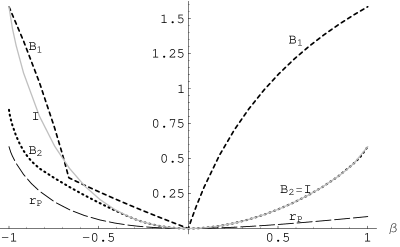
Figure 1: The dashed lines represent bounds of rate for Werner states (d=3) ($r_{\mathcal{P}}^{\rightarrow}\leq B_{2}\leq B_{1}$) and continuous line represents quantity described by $I=2\log_{2}d-S(\varrho)$. Note that $B_{2}$ is equal to information content of state in whole range of separability ($\beta\geq-\frac{1}{3}$)

Looking at Fig. 2 we can see $B_{2}$ and $r^{\rightarrow}_{\mathcal{P}}$ for some different dimensions of Hilbert space of Werner state. Continuous lines represent bounds for d=3 , the long dashed lines bounds for d=4 and the short dashed for d=5.

Figure 2: Upper bound $B_{2}$ and lower bound $r^{\rightarrow}_{\mathcal{P}}$ of rate for Werner states (d=3,4,5).

Now, let us present results for isotropic state. For these states the bound $B_{1}$ is given by:

$$B_{1}=\left\{\begin{array}[]{ll}\log_{2}[-\lambda(d+1)+1]&\textrm{for}\quad\lambda<0\\ \log_{2}[\lambda(d-1)+1]&\textrm{for}\quad\lambda\geq 0\end{array}\right.$$ (62)

Using the same arguments like for Werner state we can show that if we want to find value of $B_{2}(\varrho_{iso})$ we ought to optimize $B_{2}(\varrho_{iso},\sigma)$ on isotropic state. Analogously, as in previous case, we can find out that :

$$B_{2}=\left\{\begin{array}[]{ll}2\log_{2}d-S(\varrho_{iso})&\textrm{for}\quad\frac{-1}{d^{2}-1}\leq\lambda\leq\frac{1}{d+1}\\ 2\log_{2}d-S(\varrho_{iso})+\log_{2}\frac{1+p(d-1)}{1-p}-\frac{1+\lambda(d^{2}-1)}{d^{2}}\log_{2}\frac{1-p}{1+p(d^{2}-1)}&\textrm{for}\quad\frac{1}{d+1}\leq\lambda\leq 1\\ \end{array}\right.$$ (65)

$\textrm{where}\quad p=\frac{(d+1)\lambda-1}{(1-d^{2})(\lambda-1)+d}$. The entropy of isotropic state is given by:

$$S(\varrho_{iso})=-\frac{1+\lambda(d^{2}-1)}{d^{2}}\log_{2}\frac{1+\lambda(d^{2}-1)}{d^{2}}-\frac{(1-\lambda)(d^{2}-1)}{d^{2}}\log_{2}\frac{1-\lambda}{d^{2}}$$ (66)

Isotropic state possess similar properties like Werner states, so if we want to obtain a value of $r_{\mathcal{P}}^{\rightarrow}$ we should proceed similarly like for that family of state. Then we have

$$r_{\mathcal{P}}^{\rightarrow}=\log_{2}d+(\lambda+\frac{1-\lambda}{d})\log_{2}(1+\frac{1-\lambda}{d})$$ (67)

For isotropic state the bound $B_{2}$ is better again than $B_{1}$ and also only for entangled isotropic state the upper bound is nontrivial. The upper and lower bounds agree for $P_{+}$ and are obviously equal to $\log_{2}d$. The bounds and information content are compared on figure (3) for d=3. The upper dashed line represent $B_{2}$, the lower $\mathop{r}_{\mathcal{P}}^{\rightarrow}$. The gray continuous line is a information content of state, i.e. $2\log_{2}d-S(\varrho_{iso)}$.

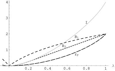
Figure 3: The dashed lines represent bounds of rate for isotropic states (d=3) and continuous line information content of state. Note that $B_{2}$ is equal to $I=2\log_{2}d-S(\varrho)$ for whole range of separability ($\lambda\leq\frac{1}{1+d}$)

.

On Figure 4 give us ability to compare quantity B2 and $\mathop{r}_{\mathcal{P}}^{\rightarrow}$ for some different dimension (d=3,4,5).

Figure 4: Upper bound B2 and lower bound $r^{\rightarrow}_{\mathcal{P}}$ of rate for isotropic states (d=3,4,5).

VI Comparison quantum deficit with measures of entanglement

As one knows that quantum deficit $\Delta$ can be treated as a measure of quantum correlations Oppenheim et al. (2002a). Having bound localisable information we can find bounds for $\Delta$. We can do this, because quantum deficit is defined as a difference between total information and information $I_{l}$, which can be localized by NLOCC (2) and we know that $I_{l}$ is bounded by information localisable by using PPT-PMM operation.

We would like to compare quantum deficit with another measure of entanglement, because we suppose that this quantity is more general measure of ”quantumness” of state that well-known measure of entanglement.

This way we get lower bound $\delta_{B}$ for $\Delta$:

$$\delta_{B}(\varrho)=2\log_{2}d-S(\varrho)-B_{2}$$ (68)

and upper bound $\delta_{P}$ :

$$\delta_{P}(\varrho)=2\log_{2}d-S(\varrho)-r^{\rightarrow}_{\mathcal{P}}$$ (69)

We can compare $\Delta$ with known measures of entanglement.
The regularized relative entropy of entanglement $E_{R}^{\infty}$ for Werner states is given by Audenaert et al. (2001):

$$E_{R}^{\infty}=\left\{\begin{array}[]{ll}\log_{2}\frac{d-2}{d}+\frac{(d-1)(1-\beta)}{2(d+\beta)}\log_{2}\frac{d+2}{d-2}&\textrm{for}\quad-1\leq\beta\leq-\frac{3d}{d^{2}+2}\\ 1+H(\frac{(d-1)(1-\beta)}{2(d+\beta)})&\textrm{for}\quad-\frac{3d}{d^{2}+2}\leq\beta\leq-\frac{1}{d}\\ 0&\textrm{for}\quad-\frac{1}{d}\leq\beta\leq 1\end{array}\right.$$ (73)

Entanglement of formation is described by the following formula:

$$E_{F}=\left\{\begin{array}[]{ll}H(\frac{1}{2}(1-\sqrt{1-(\frac{1+d\beta}{d+\beta})^{2}}\big{)}&\textrm{for}\quad-1\leq\beta\leq-\frac{1}{d}\\ 0&\textrm{for}\quad-\frac{1}{d}<\beta\leq 1\end{array}\right.$$ (76)

We can see on Fig. (5) the graphs of $\delta_{B}$ , $\delta_{P}$, $E_{F}$ and $E_{R}^{\infty}$ for Werner states. We obtain that $\delta_{B}$ and $E_{R}^{\infty}$ are equal. For Werner states with $\beta<0.42$ we have that quantum deficit is not less than entanglement of formation: $\Delta\leq E_{F}$.

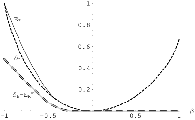
Figure 5: The dashed lines represent upper and lower bounds of $\Delta$ for Werner states (d=5), grey continuous regularized relative entropy of entanglement $E_{R}^{\infty}$ and black continuous entanglement of formation $E_{F}$.

Let us now pass to isotropic states. For entangled ones with parameter $\lambda\in(\frac{1}{d+1},1)$ the relative entropy of entanglement $E_{R}$ is given by:

$$E_{R}=\log_{2}d+f\log_{2}f+(1-f)\log_{2}\frac{1-f}{d-1}$$ (77)

where $f=\frac{(d^{2}-1)\lambda+1}{d^{2}}$. For another isotropic states it is surely zero. The formula of entanglement of formation we can find in paper K.G.H.Vollbrecht and R.F.Werner (2001). For nonseparable states it is in form of:

$$E_{F}(\varrho) = co(g(\gamma))$$ (78)

$$g(\gamma) = (H_{2}(\gamma)+(1-\gamma)\log_{2}(d-1))$$ (79)

where $\gamma=\frac{1}{d^{2}}\Big{(}\sqrt{d\lambda+\frac{1-\lambda}{d}}+\sqrt{(d-1)\frac{(d^{2}-1)(1-\lambda)}{d}}\Big{)}^{2}$ and co means a convex hull K.G.H.Vollbrecht and R.F.Werner (2001). On figure (6) we can see graphs of two measure of entanglement and bounds for delta.

We can notice that the graphs of $\delta_{B}$ agree with $E_{R}$. Similary as for Werner states we have $\delta_{B}=E_{R}$. $\delta_{P}$ is grater than $E_{F}$ for most isotropic states. (We do not know, if it is true for all isotropic states). For maximally entangled state $P_{+}$ all these quantities are equal.

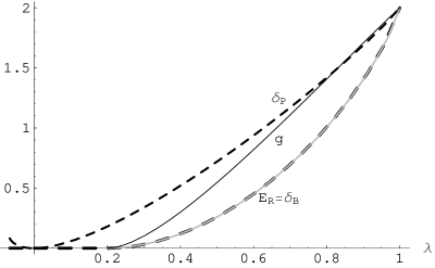
Figure 6: The dashed lines represent bounds for $\Delta$ for isotropic states (d=3), grey continuous regularized relative entropy of entanglement $E_{R}$ and black continuous $g(\gamma)$(whose convex hull is entanglement of formation $E_{F}$).

VII Fidelity for distillation of local pure states and singlets

The well known counterpart of a qubit which represents the unit of local information is ebit - one bit of entanglement, represented by singled state i.e. unit of nonlocal information. It has been stated in Oppenheim et al. (2002b) that these two forms of information are complementary. If one distills maximal possible amount of one type of information, possibility of gaining the second type disappears. The optimal protocol in case of pure initial state $\psi_{AB}^{\otimes n}$, in which both types are obtained with some ratios, has been also shown there. We will find a bound for the fidelity of such transition, in which both qubits and ebits are drawn in an NLOCC protocol in case of general mixed state $\rho_{AB}^{\otimes n}$. One can view this as a purity distillation protocol, because purity in general has two extreme forms: purely local, and purely nonlocal one. This is due to the fact, that any nonproduct pure state, is asymptotically equivalent to the singlet state under the set of NLOCC operations Horodecki et al. (2003a). To this end - as before - we will consider broader class than the NLOCC, namely the class PPT-PMM. This time we have to fix two rates: the one which tell us how many pure local qubits we would like to obtain ($r_{l}$), but also how many singlet states ($r_{s}$) will be acheived per n copies of input state (see fig. 7).

Figure 7: Scenario of distillation of pure states in their two extremal forms: purely local (product) states and purely nonlocal (maximally entangled) states. The fixed rates of transition gives the proportion of the number of input copies n of state $\rho$ to the numbers of output copies of local states ($\log K_{l}$) and singlet states ($\log K_{s}$).

Namely

$$r_{s}={\log{K_{s}}\over n},\hskip 5.69046ptr_{l}={2m-2\log{K_{s}}\over n}$$ (80)

where $n$ is the number of input states, $m$ is the number of qubits which output states occupies (both pure qubits, and singlets together) and $\log{K_{s}}$ is the output number of singlet states. We get less than $2m\over n$ pure qubits since $\log{K_{s}}$ singlets use up $2\log{K_{s}}$ qubits out of $2m$ final. We should maximize the fidelity of transition:

$$F={\rm Tr}[P_{+}^{\otimes\log K_{s}}\otimes P_{00}^{\otimes(m-\log{K_{s}})}\Lambda(\rho^{\otimes n})].$$ (81)

where $P_{+}^{\otimes\log K_{s}}$ is the projector onto the singlet state on ${\cal C}^{K_{s}}\otimes{\cal C}^{K_{s}}$. Instead of tensor product of singlets and product states, we can equally well consider the output state as the same singlet state embedded in the larger Hilbert space ${\cal C}^{m}\otimes{\cal C}^{m}$. Thus we shall maximize the following quantity:

$$F={\rm Tr}[P_{+}^{K_{s}}\Lambda(\rho^{\otimes n})].$$ (82)

where $K_{s}$ reminds that $P_{+}$ is of less dimension than the whole Hilbert space it is embedded in. The rest of the space is occupied by pure local qubits i.e. the second resource drawn in this process.

Consequently we will first consider the fidelity in terms of the $\Pi=\Lambda^{\dagger}(P^{K_{s}}_{+})$ operator where $\Lambda^{\dagger}$ is dual (hence CP) to the $\Lambda$ which is CPTP from assumption.

Analogously as in section III we can obtain the following fact

Fact 2

For given rates $r_{l}$, $r_{s}$ and the number of input copies n, the optimal fidelity is given by

$$F\leq\sup_{\Pi}{\rm Tr}[\Pi(\rho^{\otimes n})],$$ (83)

where

$$0\leq\Pi\leq{\rm I},\hskip 8.5359pt{-{\rm I}\over K_{s}}\leq\Pi^{\Gamma}\leq{{\rm I}\over K_{s}},\hskip 8.5359pt{\rm Tr}[\Pi]=2^{n(2\log d-r_{l}-2r_{s})}\equiv K.$$

Passing to dual problem, after some algebra we get

Theorem 4

For any state $\rho$ acting on $({\cal C}^{d}\otimes{\cal C}^{d})^{\otimes n}$ and rates $r_{l}$ and $r_{s}$ we have

$$F\leq\inf_{D}\{Tr(\rho-D)_{+}+\inf_{\lambda}[{1\over K_{s}}{\rm Tr}|D^{\Gamma}-\lambda{\rm I}|+\lambda K]\}$$ (84)

where infimum are taken over all hermitian operators D and all real numbers $\lambda$ respectively; $K=2^{n(2\log d-r_{l}-2r_{s})}$ and $K_{s}=2^{nr_{s}}$.

It is not easy to obtain nontrivial results. Suppose that we want to apply analogous ideas to those applied in section (IV). Let us rewrite fidelity as follows (for some fixed $D$,

$$F\leq Tr(\rho^{\otimes n}-D)+2^{-nr_{s}}{\rm Tr}|D^{\Gamma}-\lambda{\rm I}|+\lambda 2^{n(2\log d-r_{l})}$$ (85)

The simplest approach would be to force first terms to vanish , and to try to put $D=\varrho^{\otimes n}$. However, even by this simplification it is very difficult to find any bound for rates.

Yet, there are also ”higher level” problems. Namely the main problem within the connection between distillation of entanglement and the paradigm of localising information, is whether distillation process consume local information Oppenheim et al. (2003). It seems that our class of operations cannot feel this problem at all. Indeed, it is likely, that any distillation process is a map that preserve maximally mixed state jon . Thus one should perhaps improve the approach, by imposing more stringent constraints on class of operations. This is because for initial maximally mixed state, we impose only final maximally mixed state. However generically, final dimension is smaller than initial one. This means that some tracing out must take place, and we do not require the state that was traced out must be maximally mixed. Thus in our class, pure ancillas can be added, under the condition that they are finally traced out.

VIII Discussion

In this paper we have investigated localisable information and associated information deficit of quantum bipartite states. We used the fact, that localisable information can be defined as the amount of pure local qubits (per input copy) that can be distilled by use of classical communication and local operations that do not allow adding local ancilla in non-maximally mixed state. We considered a larger class of operations which we called PPT-PMM operations. They are those PPT operations which preserve maximally mixed state. Then we managed to formulate the problem of distillation of pure product qubits in terms of semidefinite program. Using duality concept in semidefinite programming we have found bound for fidelity of transition given state into pure product ones by PPT-PMM operations. In this way we obtained a general upper bound for amount of localisable information of arbitrary state. The bound was denoted $B_{2}$ (we also obtained a simpler, but weaker bound $B_{1}$). It gives bound $\delta_{B}$ for information deficit. We were able to evaluate exactly the value of the bound $B_{2}$ for states exhibiting high symmetry - Werner states and isotropic states. Quite surprisingly, the obtained related lower bound $\delta_{B}$ for information deficit turned out to coincide with relative entropy of entanglement in the case of isotropic states, and with regularized relative entropy of entanglement for Werner states. In other words: in those two cases, our bound for information deficit, turned out to be equal to Rains bound for distillable entanglement. We also analysed a simple lower bound $r_{P}$ for localisable information, and a parallel upper bound $\delta_{P}$ for information deficit. We compared the latter bound with entanglement of formation. In particular we obtained that for Werner states $(d=3)$, in entangled region it is strictly smaller than entanglement of formation. If one believes that information deficit is a measure of total quantumness of correlations, the conclusion would be that $E_{F}$ does not describe the entanglement present in state. Rather it includes also the entanglement that got dissipated during formation of the state. Finally, we also discussed possibility of application of our approach to the problem of simultaneous distillation of singlets and pure local states. We provided bound for fidelity in this case. However it is likely, that the chosen class of operations is too large to describe information consumption in the process of distillation of entanglement. We believe that our results will stimulate further research towards evaluating localisable information and information deficit. An important open question is also the connection between information deficit and entanglement measures. In particular, it is intriguing, how general is the equality of our lower bound for deficit, and $E_{r}$ - upper bound for distillable entanglement.

Acknowledgments: We thank Paweł Horodecki, Ryszard Horodecki and Jonathan Oppenheim for helpful discussion. This work is supported by EU grants RESQ, Contract No. IST-2001-37559 and QUPRODIS, Contract No. IST-2001-38877 and by the Polish Ministry of Scientific Research and Information Technology under the (solicited) grant No. PBZ-MIN-008/ P03/ 2003.

References

- Oppenheim et al. (2002a) J. Oppenheim, M. Horodecki, P. Horodecki, and R. Horodecki, Phys. Rev. Lett 89, 180402 (2002a), eprint quant-ph/0112074.
- Horodecki et al. (2003a) M. Horodecki, K.Horodecki, P.Horodecki, R. Horodecki, J. Oppenheim, A. Sen(De), and U. Sen, Phys. Rev. Lett. 90, 100402 (2003a), eprint quant-ph/0207168.
- Scully (2001) M. O. Scully, Phys. Rev. Lett 87, 220601 (2001).
- (4) V. Vedral, eprint quant-ph/9903049.
- (5) R. Alicki, M. Horodecki, P. Horodecki, and R. Horodecki, eprint quant-ph/0402012.
- Bennett et al. (1997) C. H. Bennett, D. P. DiVincenzo, and J. S. W. K. Wootters, Phys. Rev. A 54, 3824 (1997), eprint quant-ph/9604024.
- Oppenheim et al. (2002b) J. Oppenheim, K. Horodecki, M. Horodecki, P. Horodecki, and R. Horodecki (2002b), eprint quant-ph/0207025.
- Werner (1989) R. Werner, Phys. Rev. A 40, 4277 (1989).
- Horodecki and Horodecki (1999) M. Horodecki and P. Horodecki, Phys. Rev. A 59, 4206 (1999), eprint quant-ph/9708015.
- Rains (2000) E. Rains (2000), eprint quant-ph/0008047.
- (11) M.Horodecki, P.Horodecki, R.Horodecki,J.Oppenheim, A.Sen(De), U.Sen and B. Synak-In preparation.
- Rains (1999) E. Rains, Phys. Rev. A 60, 179 (1999), eprint quant-ph/9809082.
- Horodecki et al. (2003b) M. Horodecki, P. Horodecki, and J. Oppenheim (2003b), eprint quant-ph/0302139.
- (14) T. Ogawa and M. Hayashi, eprint quant-ph/0110125.
- Audenaert et al. (2001) K. Audenaert, J. Eisert, E. Jane, M. Plenio, S. Virmani, and B. D. Moor, Phys. Rev. Lett. p. 217902 (2001).
- K.G.H.Vollbrecht and R.F.Werner (2001) K.G.H.Vollbrecht and R.F.Werner, Phys. Rev. A 64, 0623074 (2001), eprint quant-ph/0010095.
- Oppenheim et al. (2003) J. Oppenheim, M. Horodecki, and R. Horodecki, Phys. Rev. Lett 90, 010404 (2003), eprint quant-ph/0207169.
- (18) We found this in discussion with J. Oppenheim.