Fault-tolerant quantum computation with cluster states

Abstract

The one-way quantum computing model introduced by Raussendorf and Briegel [Phys. Rev. Lett. 86 (22), 5188-5191 (2001)] shows that it is possible to quantum compute using only a fixed entangled resource known as a cluster state, and adaptive single-qubit measurements. This model is the basis for several practical proposals for quantum computation, including a promising proposal for optical quantum computation based on cluster states [M. A. Nielsen, arXiv:quant-ph/0402005, accepted to appear in Phys. Rev. Lett.]. A significant open question is whether such proposals are scalable in the presence of physically realistic noise. In this paper we prove two threshold theorems which show that scalable fault-tolerant quantum computation may be achieved in implementations based on cluster states, provided the noise in the implementations is below some constant threshold value. Our first threshold theorem applies to a class of implementations in which entangling gates are applied deterministically, but with a small amount of noise. We expect this threshold to be applicable in a wide variety of physical systems. Our second threshold theorem is specifically adapted to proposals such as the optical cluster-state proposal, in which non-deterministic entangling gates are used. A critical technical component of our proofs is two powerful theorems which relate the properties of noisy unitary operations restricted to act on a subspace of state space to extensions of those operations acting on the entire state space. We expect these theorems to have a variety of applications in other areas of quantum information science.

I Introduction

I.1 Overview

One of the most surprising recent developments in quantum computation is the insight that quantum measurement can be used as the fundamental dynamical operation in a quantum computer Raussendorf and Briegel (2001); Nielsen (2003a). This insight has significant implications for our theoretical understanding of how quantum computers operate, and also for the development of practical proposals for quantum computing.

Historically, the first measurement-based model for quantum computing was the one-way quantum computer developed by Raussendorf and Briegel Raussendorf and Briegel (2001). A one-way quantum computation is performed in two stages. In the first stage an entangled many-qubit state known as the cluster state is prepared. This is a fixed entangled state that does not depend on the problem instance being solved by the computation. Indeed, when the one-way quantum computation is being used to simulate a quantum circuit, Raussendorf and Briegel (2001) shows that the identity of the cluster state can be made very nearly independent of the details of the circuit being simulated, with the only dependence being on the depth and breadth of the circuit. In the second stage of a one-way quantum computation a sequence of single-qubit measurements is performed on the cluster state. These measurements are adaptive, in the sense that the basis in which a qubit is measured may depend upon the outcome of earlier measurements. Remarkably, this two-stage process is sufficient to simulate any quantum circuit whatsoever.

More recently, an apparently quite different teleportation-based Bennett et al. (1993) approach to measurement-based quantum computation was developed by Nielsen Nielsen (2003a). This approach is based on the idea now known as gate teleportation, introduced by Nielsen and Chuang Nielsen and Chuang (1997), and further developed by Gottesman and Chuang Gottesman and Chuang (1999). When it was first introduced, teleportation-based quantum computation appeared to be quite different from the one-way quantum computer, but subsequent work Aliferis and Leung (2004); Jorrand and Perdrix (2004); Childs et al. (2004) has provided a unified conceptual framework in which both approaches may be understood.

Although the measurement-based models of quantum computation represent an important conceptual advance, there is an important caveat, namely, that the measurement-based models assume all operations are carried out perfectly. Since real physical systems suffer from noise, to make measurement-based models scalable we must develop techniques for combatting noise in those models.

The challenge posed by noise has been met in the quantum circuit model of computation with the development of an impressive theory of fault-tolerance, providing a large body of techniques which can be used to reduce the effects of noise on quantum circuits. The culmination of the theory of fault-tolerance is the threshold theorem, which states that for physically reasonable models of noise, and provided the noise is below some constant threshold value, it is possible to use quantum circuits to efficiently simulate an arbitrarily long quantum computation with arbitrary accuracy. Although the threshold remains to be experimentally confirmed, there is now general agreement that, based on our best theoretical understanding of quantum noise, the threshold theorem solves the problem of noise in the quantum circuit model of computation. That is, quantum noise poses no problem of principle for quantum computation, only the (very significant) practical problem of reducing noise levels below the threshold value. For a survey of the theory of fault-tolerance and the threshold theorem see Chapter 10 of Nielsen and Chuang (2000), and references therein.

The purpose of the present paper is to develop similar fault-tolerant threshold results for several measurement-based models of quantum computation, focusing primarily on models derived from the one-way quantum computer of Raussendorf and Briegel. We refer to this entire class of models as the cluster-state model of quantum computation, to emphasize the crucial role played by cluster states. Note that we use the term “cluster-state model of quantum computation” in a rather loose sense, using it to denote an entire class of models based on cluster states. We reserve the term one-way quantum computer to refer to the specific model originally suggested in Raussendorf and Briegel (2001).

Our primary motivation in studying fault-tolerance in the cluster-state model is to establish that the cluster-state model can be used as the basis for scalable practical proposals for quantum computation. Although several proposals for experimental quantum computation with cluster states have been made Raussendorf and Briegel (2001); Nielsen (2004), such proposals cannot be considered scalable unless fault-tolerant methods of implementation are developed. In this paper we develop methods for fault-tolerant computation using cluster states, methods that are applicable in a wide variety of practical proposals.

Prior work on the problem of fault-tolerant computation with cluster states has been reported in Chapter 4 of Raussendorf’s thesis Raussendorf (2003). This work obtained a threshold for a class of noise models in which Pauli errors occur probabilistically in a cluster-state computation. Our threshold result applies to a more general noise model that is likely to be more realistic in many physical systems; subject to some assumptions about locality, we allow arbitrary non-Markovian noise to occur in the computation, and even allow errors to occur in the accompanying classical computation. Thus, our work should be viewed as extending and complementing the approach taken in Raussendorf (2003). We note that independent work extending Raussendorf (2003) is also being undertaken by Raussendorf and Briegel Raussendorf and Briegel .

What is it that makes proving a fault-tolerant threshold in the cluster-state model non-trivial? The obvious approach to proving a threshold is to take the quantum circuit that we want to make fault-tolerant, convert it to a fault-tolerant quantum circuit using the standard prescriptions, and then simulate the resulting circuit using a cluster-state computation. It seems physically plausible that noise occurring in the cluster-state model of computation should then be corrected by the error-correcting properties of the original fault-tolerant circuit.

Two difficulties obstruct this proposal. The first difficulty is that the qubits in the cluster tend to degrade before they are measured. We will see that this difficulty can easily be overcome by building up the cluster in parts, so that no part of the cluster is allowed to degrade too much before being measured.

The second difficulty is more serious. While it is plausible that noise in the cluster-state computation is corrected by the error-correcting properties of the original fault-tolerant circuit, showing this turns out to be non-trivial. The key is to prove that noise in a cluster-state simulation of a quantum circuit can be mapped onto equivalent noise in the quantum circuit. Provided that mapping has suitable properties, a threshold theorem then follows. The greater part of this paper is spent in constructing such a mapping. To underscore the difficulty in proving this, we mention just one interesting subtlety: we shall see that Markovian noise in a cluster-state computation actually maps onto non-Markovian noise in the corresponding quantum circuit. This and other subtleties make the task of proving a threshold technically challenging.

This discussion highlights a general point worth noting. Our paper provides a way of taking an arbitrary quantum circuit and then simulating it in a fault-tolerant fashion in the cluster-state model of computation. We don’t, however, provide a direct way of making a cluster-state computation fault-tolerant, except insofar as a cluster-state computation may be regarded as a special type of quantum circuit computation. It would be interesting to investigate more direct fault-tolerance constructions applicable to an arbitrary cluster-state computation. Of course, for the purposes of proving the feasibility of scalable quantum computation in the cluster-state model, the present approach is sufficient.

I.2 Optical cluster states and fault tolerance

A topic of special interest in the present paper is the optical cluster-state proposal for quantum computation suggested by Nielsen Nielsen (2004). Optical systems offer a number of significant experimental advantages for quantum computing, and this proposal thus offers a very promising approach to experimental quantum computation. However, the optical cluster-state proposal also differs from most quantum computing proposals in that it is based on entangling gates that only work non-deterministically. This non-deterministic nature poses special difficulties when attempting to prove a threshold for the optical cluster-state proposal. Following Nielsen (2004), we now briefly review some background on this proposal that will help the reader understand how it fits into the present paper.

A priori, optics offers significant advantages for the implementation of quantum computation, such as the ease of performing basic manipulations, and long decoherence times. Unfortunately, standard linear optical elements alone are unsuitable for quantum computation, as they do not enable photons to interact. This difficulty can, in principle, be resolved by making use of nonlinear optical elements Yamamoto et al. (1988); Milburn (1989), at the price of requiring large nonlinearities that are at present extremely difficult to achieve.

An alternate approach was developed by Knill, Laflamme and Milburn (KLM) Knill et al. (2001), who proposed using measurement to effect entangling interactions between optical qubits. Using this idea, KLM developed a scheme for scalable quantum computation based on linear optical elements, together with high-efficiency photodetection, feedforward of measurement results, and single-photon generation. KLM thus showed that scalable optical quantum computation is in principle possible using relatively modest resources. Experimental demonstrations Pittman et al. (2003); O’Brien et al. (2003); Sanaka et al. (2003); Gasparoni et al. (2004); Zhao et al. (2004) of several of the basic elements of KLM have already been achieved.

Despite these impressive successes, the obstacles to fully scalable quantum computation with KLM remain formidable. The biggest challenge is to perform a two-qubit entangling gate in the near-deterministic fashion required for scalable quantum computation. KLM propose doing this using a combination of three ideas. (1) Using linear optics, single-photon sources and photodetectors, non-deterministically perform an entangling gate. This gate fails most of the time, destroying the state of the computer when it does so, and so is not immediately suitable for quantum computation. Several variants of this gate have already been experimentally demonstrated Pittman et al. (2003); O’Brien et al. (2003); Sanaka et al. (2003); Gasparoni et al. (2004); Zhao et al. (2004). (2) By combining the basic non-deterministic gate with quantum teleportation, a class of non-deterministic gates which are not so destructive of the state of the computer is found. (3) By combining the gates from (2) with ideas from quantum error-correction, the probability of the gate succeeding can be improved until the gate is near-deterministic, allowing scalable quantum computation.

The combination of these three ideas allows scalable quantum computation, in principle. In practice there are enormous obstacles to performing even a single near-deterministic entangling quantum gate in this fashion. The proposal of Nielsen (2004) eliminates much of the difficulty, completely removing step (3), and obviating the need for all but the simplest versions of step (2). This is achieved by combining some of the simplest elements of KLM with the cluster-state model of quantum computation. The resulting proposal puts near-deterministic entangling quantum gates within experimental reach, and thus offers an extremely promising approach to quantum computation, provided suitable methods for dealing with noise can be developed.

I.3 Content of the paper

In this paper we prove two threshold theorems for cluster-state quantum computation. The first is a general threshold theorem applicable to a variety of possible implementations of cluster-state computation, assuming that deterministic entangling gates are available. The second is specifically adapted to the optical cluster-state proposal for quantum computation. Taken together, these theorems show that for a wide variety of possible physical implementations, noise poses no problem of principle for fully scalable cluster-state quantum computation.

Before describing in detail the structure of the paper, it is worth noting two issues that we do not fully address. The first of these issues is the determination of a numerical value for the threshold. Although we do obtain bounds on the threshold, those bounds are obtained through analytic methods that are far too pessimistic. Our philosophy is that the problem of understanding the threshold is best split into two parts. In the first part, one attempts to rigorously prove the existence of a finite threshold for some large class of noise models. In the second part, one attempts through a combination of numerical and analytic work to obtain a realistic estimate of the threshold for some specific and physically-motivated noise model. In this second part it is much more reasonable to rely on numerical evidence and heuristic reasoning, since results for specific noise models can always be checked by computer simulation (and ultimately by experiment). Examples of this kind of work for quantum circuits may be found in Knill (2004a, b); Steane (2002); Steane and Ibinson (2003); Dür and Briegel (2003), and references therein. Our focus in the present paper has been on the first part of this program, obtaining a rigorous proof that a finite threshold exists. Detailed numerical simulation and optimization of the threshold value for realistic noise models is underway, and will be reported elsewhere Dawson et al. .

The second issue not fully addressed in this paper relates to the noise model used in our analysis of the optical cluster-state proposal for quantum computation. Physically, one of the most significant sources of noise in any optical implementation is likely to be photon loss. This causes the state of the optical qubit to “leak” from the degrees of freedom associated with the qubit out into some other dimensions of the physical state space. In the context of threshold theorems, such noise is known as a “leakage error”, and there are standard techniques for dealing with such errors in the theory of fault-tolerance. However, our threshold analysis for the cluster-state model is based on the recent threshold theorem proved by Terhal and Burkard Terhal and Burkard (2004), and that threshold does not explicitly deal with leakage errors. While it seems extremely likely to us that the result of Terhal and Burkard (2004) can be patched so that leakage errors are accounted for, we have not worked through the analysis in detail. Rather than do so, in this paper we restrict ourselves to a brief discussion of leakage, deferring full investigation of this issue to a future publication. The other alternative, of course, would be to base our analysis on an alternative version of the threshold theorem. However, we will see that the theorem of Terhal and Burkard has considerable advantages for the analysis of fault-tolerance with cluster states, as the only published version of the threshold formulated specifically to deal with non-Markovian noise.

The structure of the paper is as follows. We begin in Section II by defining a measure of how much noise occurs in a quantum information processing task. We call this measure the error strength, and prove several simple properties of the error strength that will be useful later in the paper.

Section II also contains two important technical results, which we dub the first and second unitary extension theorems. Roughly speaking, these results are applicable to situations in which two unitary operations $U$ and $V$ act in a similar fashion on a subspace $S$ of state space. Of course, just because $U$ and $V$ act similarly on a subspace, it does not follow that they have similar global actions on state space. However, the theorems we prove guarantee that there exist unitary extensions $\tilde{U}$ and $\tilde{V}$ of the restrictions $U|_{S}$ and $V|_{S}$, respectively, such that $\tilde{U}$ and $\tilde{V}$ have approximately equal actions everywhere on state space. These unitary extension theorems are critical to our later analysis of fault-tolerance. More generally, we believe that these results are of substantial interest independent of their application to fault-tolerance, and likely to find application in other areas of quantum information science.

Section II concludes with a review of the content of the threshold theorem for quantum circuits. We focus our attention on the threshold theorem proved recently by Terhal and Burkard Terhal and Burkard (2004), extending earlier work of Aharonov and Ben-Or Aharonov and Ben-Or (1997, 1999). The threshold of Terhal and Burkard (2004) is unique in that it is specifically designed with non-Markovian noise in mind. While several of the other known variants of the threshold theorem can cope with some level of non-Markovian noise, those other variants are designed primarily with the case of Markovian noise in mind. This is important for us as we will see that non-Markovian noise arises naturally in the analysis of fault-tolerant cluster-state quantum computation, even if the actual physical noise occurring in the cluster-state computation is Markovian.

In Section III we describe the cluster-state model of quantum computation. Rather than providing a detailed proof of how the model works (which is available elsewhere) we describe the model through some simple examples. We also discuss ways of alleviating one of the key difficulties that arises when attempting to perform fault-tolerant quantum computation with cluster states, the tendency of qubits in the cluster to degrade before they are measured. We conclude with a brief review of how the cluster-state model of quantum computation can be combined with the ideas of KLM to obtain a scheme for optical quantum computation.

Section IV is the heart of the paper, stating and proving our first threshold theorem for cluster-state computation. More precisely, what we prove is that it is possible to simulate an arbitrary quantum circuit using a noisy cluster-state computation, with arbitrary accuracy and only a small overhead in the physical resources required, subject to reasonable constraints on the physical resources available, and on the noise afflicting the implementation.

The sequence of ideas used to prove this threshold theorem is conceptually rather simple. Step one is to translate the quantum circuit that we want to simulate into a fault-tolerant circuit, using the standard prescriptions for making a circuit fault-tolerant. At this stage we assume there is no noise in the computation. Step two is to translate the fault-tolerant circuit into a cluster-state computation, again using standard prescriptions. Step three is to carefully specify a procedure for physically implementing the cluster-state computation, a procedure that avoids the degradation of parts of the cluster that was mentioned above. The idea is to build up only part of the cluster at any given time, adding extra qubits into the cluster as required. Up until this step we assume that all operations are perfect. Step four is to introduce noise into the description of the cluster-state computation, as would occur in an actual implementation. The most complex and critical step, step five, is to show that the noisy cluster-state computation is equivalent to the original fault-tolerant circuit, with some noise added into the circuit. That is, we want to map noise in the cluster-state computation back onto equivalent noise in the original fault-tolerant circuit. We will see that this mapping has the property that provided the noise in the cluster-state model is of an appropriate form, and not too strong, it is equivalent to noise in the original fault-tolerant circuit which is only slightly stronger, and which is of a form which can be suppressed by the usual fault-tolerance constructions for quantum circuits. This mapping of noise models thus enables us to infer a threshold theorem for noisy cluster-state computation.

Section V extends these ideas to the optical cluster-state proposal for quantum computation. The reason the results of Section IV cannot be immediately applied is that the entangling gates used in the optical cluster-state proposal are non-deterministic. We resolve this problem by devising an approach to computation in which the non-deterministic entangling gates can be treated as deterministic entangling gates, subject to a small amount of additional noise. This enables us to map noise in the optical cluster-state proposal into equivalent noise in the deterministic cluster-state model, and then use the result of Section IV to infer a threshold theorem for optical cluster-state quantum computation.

Section VI concludes the paper with a summary of results, and a discussion of the outlook for further developments.

II Noise and fault-tolerant quantum circuits

In order to prove a threshold for cluster-state computation we first need a way of describing quantum noise, and quantifying its effects. In Subsection II.1 we introduce a measure that quantifies the effects of quantum noise, describe some properties of that measure, and describe the unitary extension theorems. In Subsection II.2 we review the threshold theorem for quantum circuits proved by Terhal and Burkard Terhal and Burkard (2004).

II.1 Error strength

Suppose we have a quantum system, $Q$, and we wish to implement a unitary operation $U_{Q}$ on that system. Unfortunately, the system is not completely isolated from its environment, $E$, and thus the true evolution of the system will be described by some unitary evolution $V_{QE}$ acting on both the system and the environment. We define the error strength or noise strength of this operation by:

$$\Delta_{Q:E}(U_{Q},V_{QE}) \equiv \min_{U_{E}}\|V_{QE}-U_{Q}\otimes U_{E}\|,$$ (1)

where the minimum is over all unitary operations $U_{E}$ on the system $E$, and the norm is the usual operator norm.

We will use the error strength $\Delta_{Q:E}$ as our principal measure of noise in the implementation of quantum computation, whether it be by cluster-state methods, or by quantum circuits. Although $\Delta_{Q:E}$ has been defined only when the ideal operation $U_{Q}$ is unitary, we’ll see later that it can also be used to understand noise in operations that may not be unitary, such as measurement and state preparation. Our main reason for using the measure $\Delta_{Q:E}$ is that it is the same measure that Terhal and Burkard use in their study of fault-tolerance Terhal and Burkard (2004) for non-Markovian noise models. We now describe several properties of $\Delta_{Q:E}$ that are useful later in the paper.

Proposition 1

(Chaining property) Let $U_{Q}^{1},\ldots,U_{Q}^{m}$ be unitary operations on the system $Q$, and $V_{QE}^{1},\ldots,V_{QE}^{m}$ be unitary operations on the combined system $QE$. Then

$$\Delta_{Q:E}(U_{Q}^{1}\ldots U_{Q}^{m},V_{QE}^{1}\ldots V_{QE}^{m}) \leq \sum_{j=1}^{m}\Delta_{Q:E}(U_{Q}^{j},V_{QE}^{j}).$$

The chaining property tells us that the total error strength of a sequence of imperfect operations is less than or equal to the sum of the individual error strengths. We note that this proposition and its proof is similar to Lemma 1 in Section 1.3 of Terhal and Burkard (2004).

Proof: Choose $U_{E}^{j}$ so that $\Delta_{Q:E}(U_{Q}^{j},V_{QE}^{j})=\|V_{QE}^{j}-U_{Q}^{j}\otimes U_{E}^{j}\|$, and define $\Delta^{j}\equiv V_{QE}^{j}-U_{Q}^{j}\otimes U_{E}^{j}$. A straightforward induction on $m$ can be used to establish the formula

$$V_{QE}^{1}\ldots V_{QE}^{m} = \left(U_{Q}^{1}\ldots U_{Q}^{m}\right)\otimes\left(U_{E}^{1}\ldots U_{E}^{m}\right)$$ (3)

$$+\sum_{j=1}^{m}\left(U_{Q}^{1}\ldots U_{Q}^{j-1}\otimes U_{E}^{1}\ldots U_{E}^{j-1}\right)\times$$

$$\hphantom{+\sum_{j=1}^{m}}\Delta^{j}\,V_{QE}^{j+1}\ldots V_{QE}^{m}.$$

The result follows by subtracting $\left(U_{Q}^{1}\ldots U_{Q}^{m}\right)\otimes\left(U_{E}^{1}\ldots U_{E}^{m}\right)$ from both sides of Eq. (3), and applying the triangle inequality.

QED

Later in the paper we will show that a noisy cluster-state computation is equivalent to a noisy quantum circuit computation. A technique we’ll use in the proof of this fact is to change the set of systems considered to be part of the environment. The following two propositions help us understand the behaviour of the error strength when the environment is changed in this way.

Proposition 2

Let $A,B$ and $C$ be three quantum systems, and let $U_{A},U_{B},V_{ABC}$ be unitary operations acting on systems indicated by the respective subscripts. Then

$$\Delta_{A:BC}(U_{A},V_{ABC})\leq\Delta_{AB:C}(U_{A}\otimes U_{B},V_{ABC}).$$ (4)

Proof: The proof is immediate from the definition of $\Delta_{Q:E}$ and the fact that the set of unitary matrices $U_{BC}$ on $BC$ is a superset of the set of unitary matrices of the form $U_{B}\otimes U_{C}$, where $U_{B}$ is the (fixed) given matrix:

$$\Delta_{A:BC}(U_{A},V_{ABC}) = \min_{U_{BC}}\|V_{ABC}-U_{A}\otimes U_{BC}\|$$

$$\leq \min_{U_{C}}\|V_{ABC}-U_{A}\otimes U_{B}\otimes U_{C}\|$$

$$= \Delta_{AB:C}(U_{A}\otimes U_{B},V_{ABC}).$$ (7)

QED

Proposition 3

Let $A,B$ and $C$ be three quantum systems, and let $U_{A},V_{AB},V_{C}$ be unitary operations acting on systems indicated by the respective subscripts. Then

$$\Delta_{A:BC}(U_{A},V_{AB}\otimes V_{C})\leq\Delta_{A:B}(U_{A},V_{AB}).$$ (8)

Proof: Similarly to the proof of the previous proposition, the proof is immediate from the definitions and the fact that the set of unitary matrices $U_{BC}$ on $BC$ is a superset of the set of unitary matrices of the form $U_{B}\otimes V_{C}$, where $V_{C}$ is the (fixed) given matrix:

$$\Delta_{A:BC}(U_{A},V_{AB}\otimes V_{C})$$ (9)

$$= \min_{U_{BC}}\|V_{AB}\otimes V_{C}-U_{A}\otimes U_{BC}\|$$

$$\leq \min_{U_{B}}\|V_{AB}\otimes V_{C}-U_{A}\otimes U_{B}\otimes V_{C}\|$$ (10)

$$= \min_{U_{B}}\|V_{AB}-U_{A}\otimes U_{B}\|$$ (11)

$$= \Delta_{A:B}(U_{A},V_{AB}).$$ (12)

QED

The next proposition helps in commuting noisy operations past one another.

Proposition 4

Let $U_{Q}$ and $V_{Q}$ be commuting unitary operations on a quantum system $Q$. Let $U_{QE}$ and $V_{QE}$ be noisy versions of these operations involving also an environment $E$. Then there exist unitaries $\tilde{U}_{QE}$ and $\tilde{V}_{QE}$ such that (a) $\tilde{U}_{QE}\tilde{V}_{QE}=V_{QE}U_{QE}$; $\Delta_{Q:E}(U_{Q},\tilde{U}_{QE})\leq\Delta_{Q:E}(V_{Q},V_{QE})$; and $\Delta_{Q:E}(V_{Q},\tilde{V}_{QE})\leq\Delta_{Q:E}(U_{Q},U_{QE})$.

This proposition tells us that if $U_{Q}$ and $V_{Q}$ commute, then applying a noisy version of $U_{Q}$ followed by a noisy version of $V_{Q}$ is equivalent to applying a noisy version of $V_{Q}$ followed by a noisy version of $U_{Q}$. Furthermore, the noise strengths in the new versions of $U_{Q}$ and $V_{Q}$ are no worse than in the originals, except for interchanging the role of $U_{Q}$ and $V_{Q}$.

Proof: Using the definition of $\Delta_{Q:E}$ we may choose unitaries $U_{E}$ and $V_{E}$, and matrices $\Delta_{U}$ and $\Delta_{V}$, such that

$$U_{QE} = (U_{Q}\otimes U_{E})(I+\Delta_{U});$$ (13)

$$\|\Delta_{U}\| = \Delta_{Q:E}(U_{Q},U_{QE});$$ (14)

$$V_{QE} = (I+\Delta_{V})(V_{Q}\otimes V_{E});$$ (15)

$$\|\Delta_{V}\| = \Delta_{Q:E}(V_{Q},V_{QE}).$$ (16)

With these choices, $I+\Delta_{U}$ and $I+\Delta_{V}$ are easily verified to be unitary operations on $QE$. We see that

$$V_{QE}U_{QE} = (I+\Delta_{V})(V_{Q}\otimes V_{E})(U_{Q}\otimes U_{E})(I+\Delta_{U})$$

$$= (I+\Delta_{V})(U_{Q}\otimes V_{E})(V_{Q}\otimes U_{E})(I+\Delta_{U}),$$

where we used the commutativity of $U_{Q}$ and $V_{Q}$ in the second line. The proof is completed by choosing $\tilde{U}_{QE}\equiv(I+\Delta_{V})(U_{Q}\otimes V_{E})$ and $\tilde{V}_{QE}\equiv(V_{Q}\otimes U_{E})(I+\Delta_{U})$.

QED

To prove our threshold theorems for cluster-state computation, we need two other theorems, which we call the first and second unitary extension theorems. These results are not phrased directly in terms of the error strength $\Delta_{Q:E}$, but we shall see later in the paper that these theorems have significant implications for the error strength.

The first unitary extension theorem may be motivated by the following problem. Suppose $V$ is a noisy unitary operation approximating a noiseless unitary operation $U$. (Note that $U$ and $V$ here act on the same state space; $U$ might correspond to $U_{Q}\otimes U_{E}$ in our earlier notation, with $V$ corresponding to $V_{QE}$.) For some physical reason we are only interested in the action of $U$ and $V$ on some subspace $S$ of the total Hilbert space. That is, we know on physical grounds that all inputs to the operations are constrained to be in that subspace. Furthermore, there is another unitary operation $\tilde{U}$ which acts identically to $U$ on the subspace $S$. A natural question is whether we can find a unitary operation $\tilde{V}$ which acts identically to $V$ on the subspace $S$, and so that $\tilde{V}$ approximates $\tilde{U}$ at least as well as $V$ approximates $U$.

Remarkably, such an extension $\tilde{V}$ always exists, and the proof of the first unitary extension theorem shows how it may be constructed. We believe this theorem has considerable independent interest in its own right, quite apart from the applications later in this paper to fault-tolerant computation with cluster states.

Theorem 1

(First unitary extension theorem) Let $U,\tilde{U}$ and $V$ be unitaries acting on a Hilbert space $T$. Suppose $S$ is a subspace of $T$ such that $U$ and $\tilde{U}$ have the same action on $S$, i.e., $U|_{S}=\tilde{U}|_{S}$. (Note that we do not assume that $U$ and $\tilde{U}$ leave the subspace $S$ invariant, so $U|_{S}$ and $\tilde{U}|_{S}$ should be considered as maps from $S$ into $T$.) Then there exists a unitary extension $\tilde{V}$ of $V|_{S}$ to the entire space $T$ such that

$$\|\tilde{V}-\tilde{U}\|\leq\|V-U\|.$$ (19)

The proof of this theorem is given in Appendix A.

The second unitary extension theorem answers a question similar in spirit, but not identical, to the question answered by the first unitary extension theorem. Let $U$ and $V$ be unitary operations acting on a vector space $T$, with a subspace $S$. Suppose $U|_{S}$ and $V|_{S}$ are close, i.e., $\|U|_{S}-V|_{S}\|$ is small. Can we argue that there exists a unitary operation $\tilde{V}$ extending $V|_{S}$, and such that $\|U-\tilde{V}\|$ is also small? The second unitary extension theorem shows that this is always true.

Theorem 2

(Second unitary extension theorem) Let $U$ and $V$ be unitary operation acting on a (finite-dimensional) inner product space $T$. Suppose $S$ is a subspace of $T$. Then there exists a unitary operation $\tilde{V}$ such that $\tilde{V}|_{S}=V|_{S}$ and

$$\|U-\tilde{V}\|\leq 2\|U|_{S}-V|_{S}\|.$$ (20)

The proof of the second unitary extension theorem is given in Appendix A. Note that this theorem may easily be restated in the language of isometries, if that is more to one’s taste. It is also worth noting that the second unitary extension theorem implies a weaker version of the first unitary extension theorem. In the notation of the first theorem, the second theorem implies that there exists a unitary extension $\tilde{V}$ of $V|_{S}$ such that $\|\tilde{V}-\tilde{U}\|\leq 2\|\tilde{U}|_{S}-V|_{S}\|\leq 2\|U-V\|$.

II.2 Fault-tolerance in the quantum circuit model

The threshold for cluster-state computation proved in this paper is based on the threshold for quantum circuits proved by Terhal and Burkard Terhal and Burkard (2004). In this subsection we review Terhal and Burkard’s result. We begin with a description of the assumptions they make about quantum circuits, including the noise model, before stating their main theorem. Note that the noise model used by Terhal and Burkard is the basis for our noise model for cluster-state computation, described in Subsection IV.1.

Terhal and Burkard split the total system up into three types of subsystem. First, there are register qubits, which can be controlled and used for computation. These qubits are present through the entirety of the computation. Second, there are ancilla qubits, which may also be controlled and used for the computation. The difference between register and ancilla qubits is that the ancillas may be brought into the computer partway through a computation, used as part of the subsequent computation, and then discarded at some later time. The third type of system is the environment, which is not under control.

The computation is represented by a sequence of unitary operations. Ideally, these operations would be applied just to the register and ancilla qubits, but inevitably they involve some interaction with the uncontrolled environment. It is this interaction which causes noise in the computer. We will find it convenient to assume the interaction with the environment is unitary; by making the environment sufficiently inclusive the laws of quantum mechanics ensure we may always make such an assumption.

Within this framework, our noise model may be described as follows. Each qubit in the computer, whether a register qubit or an ancilla qubit, has associated with it its own environment. So, for example, if we label the qubits $Q_{1},Q_{2},\ldots$, then the corresponding environments would be labeled $E_{1},E_{2},\ldots$. The key assumption we make about noise is that non-interacting qubits have non-interacting environments. More precisely, suppose as part of the computation we want to attempt some unitary gate $U$ on qubit $Q_{j}$. This might be the identity gate, representing quantum memory, or it might be a more complex gate, like a Hadamard or Pauli gate. In reality, this gate will be noisy, due to interactions with the environment. Our assumption is that the real noisy operation is a unitary evolution $V$ acting on $Q_{j}$ and its environment $E_{j}$, with the other qubits and their environments not affected. In a similar way, if we attempt a two-qubit operation $U$ between qubits $Q_{j}$ and $Q_{k}$, we assume that the real noisy evolution $V$ may involve the qubits $Q_{j},Q_{k}$, and the corresponding environments $E_{j},E_{k}$, but not the other qubits or their environments. With these assumptions, we say the noise in a noisy circuit is of strength at most $\eta$ if each ideal gate $U_{j}$ in the circuit is approximated by a noisy gate $V_{j}$ such that $\Delta_{Q:E_{Q}}(U_{j},V_{j})\leq\eta$, where $Q$ is the qubit or qubits involved in the gate, and $E_{Q}$ is the corresponding environment or environments.

We refer to the assumption that non-interacting qubits have non-interacting environments as the locality assumption for noise. Physically, the motivation for the locality assumption is that each environment is well-localized in space, and that environments can only interact with one another when two qubits are brought together to interact in a quantum gate.

Importantly, Terhal and Burkard do not make any Markovian assumption. That is, each environment can have an arbitrarily long memory. So, for example, we may perform a sequence of gates in which $Q_{1}$ first interacts with $E_{1}$, which then passes information onto $E_{2}$ through a subsequent gate, then onto $E_{3}$ through another gate, and finally corrupts qubit $Q_{4}$, say. This is in contrast with many other variants of the threshold theorem, where Markovian noise is assumed, i.e., qubits are assumed to have independent and memoryless environments.

In addition to the locality assumption for noise, Terhal and Burkard make three important additional assumptions about how quantum circuits are performed:

1. It is possible to perform quantum gates on different qubits in parallel. Physically, this requirement is due to the fact that error-correction must constantly be performed on all the qubits, even if one is merely attempting to maintain them in memory. It is possible to prove that parallelizability is a necessary condition for a threshold theorem to apply.

2. It is possible to initialize fresh ancilla qubits in the state $|0\rangle$ just prior to their being brought into the computation. Physically, this requirement is due to the fact that the ancillas are used as an entropy sink to remove noise from the computation. To be effective in this capacity they must start in a low-entropy state. It is possible to prove that the requirement for fresh ancillas is a necessary condition for a threshold theorem to apply Aharonov et al. (1996).

3. Excepting ancilla preparation, all dynamical operations applied during the computation are unitary, up until the final measurement at the end of the computation. This is not a necessary feature of a threshold theorem, but is a feature of the threshold of Terhal and Burkard.

The third assumption, that the computation is performed using only unitary operations, is rather inconvenient from our point of view, since the cluster-state model of quantum computation inherently involves many measurements performed during the computation. One feature of our proof is that it involves the replacement of measurements and classical feedforward by equivalent unitary operations. The reason we use the all-unitary model is that we need a threshold theorem which allows non-Markovian noise, and at present this means using Terhal and Burkard’s all-unitary model. Future improvements to the threshold theorem for cluster states may come by developing threshold results for quantum circuits which allow both non-Markovian noise and measurement during the computation.

To conclude preparation for the statement of the threshold theorem we need a few final items of notation and nomenclature. It will be convenient to assume that each unitary operation performed during the computation takes the same amount of time, $\Delta t$, and so the circuit may be written as a sequence of unitary operations performed at times $t=0,t=\Delta t,t=2\Delta t$, and so on. We define a location in the circuit to be specified by a triple $(k\Delta t,U,Q)$ consisting of the time $k\Delta t$ at which the gate $U$ is performed on a qubit or ordered pair of qubits, $Q$. Our measure of the total size of the circuit is the total number of locations in that circuit. Note that it is important to count locations at which the identity gate is applied to a qubit.

Computation is concluded by measuring the computer in the computational basis to produce a probability distribution $p$. The goal of fault-tolerance is to take a perfect quantum circuit which outputs a probability distribution $p$ and to construct a fault-tolerant quantum circuit that may be subject to noise, but nonetheless outputs a probability distribution $p^{\prime}$ which is close to $p$ in some suitably defined sense. As the measure of closeness we use the Kolmogorov distance, $\|p-p^{\prime}\|_{1}\equiv\frac{1}{2}\sum_{x}|p(x)-p^{\prime}(x)|$.

Theorem 3

(Threshold theorem for quantum circuits Terhal and Burkard (2004)) There exists a constant threshold $\eta_{\rm th}>0$ for quantum circuit computation with the following property. Let $n$ be the number of locations in a perfect quantum circuit, $C$, which outputs the probability distribution $p$. Let $\epsilon>0$. We can efficiently construct a noisy quantum circuit, $C^{\prime}$, with a total number of locations $n\mbox{polylog}(n^{2}/\epsilon)$, and such that if the noise in $C^{\prime}$ satisfies the locality assumption and is of strength at most $\eta_{\rm th}$ then the output distribution $p^{\prime}$ from $C^{\prime}$ satisfies $\|p-p^{\prime}\|_{1}\leq\epsilon$.

Terhal and Burkard’s construction of $C^{\prime}$ is based on a particular type of quantum error-correcting code dubbed a computation code by Aharonov and Ben-Or (definition number 15 in Aharonov and Ben-Or (1999)). As a consequence of this construction, the circuit $C^{\prime}$ is built up out of a special restricted class of quantum gates, gates that can be implemented in a fault-tolerant manner. For example, it is possible to construct $C^{\prime}$ using just operations from the following restricted set: preparation of qubits in the state $|0\rangle$; the identity gate, i.e., quantum memory; $H$ (Hadamard) gates, $Z_{\pi/4}$ and $Z_{\pi/8}$ gates, where $Z_{\theta}$ is the rotation of a single qubit by $\theta$ about the $z$ axis of the Bloch sphere; and controlled-not gates. As noted earlier, $C^{\prime}$ does not include any measurement or classical processing of data, except at the output; all dynamical operations are fully unitary.

For our purposes in this paper it is convenient to replace $C^{\prime}$ with an equivalent circuit, $C^{\prime\prime\prime}$, built up from a different set of basic operations. We make this replacement in two stages. The first stage is to replace the operations in the circuit $C^{\prime}$ by operations from the following set: preparations of a qubit in the state $|+\rangle$; the identity gate; gates of the form $X_{\alpha}Z_{\beta}$; and the controlled-$Z$ gate, which we shall call cphase. That this can always be done follows from well-known quantum circuit identities. We call the resulting circuit $C^{\prime\prime}$.

The second stage is to replace the operations in $C^{\prime\prime}$ by operations from the following set: preparations of a qubit in the state $|+\rangle$; gates of the form $HZ_{\alpha}$; and the gate $(H\otimes H)$cphase. We refer to this as the canonical set of allowed operations. To see that this can be done requires a little care, due to the absence of the identity gate from the canonical set. The trick is to simulate each gate in $C^{\prime\prime}$ by two gates from the canonical set, as follows: $I\rightarrow HH$; $X_{\alpha}Z_{\beta}\rightarrow HZ_{\alpha}HZ_{\beta}$; cphase$\rightarrow(H\otimes H)(H\otimes H)$cphase.

We call the circuit that results when these substitutions are made $C^{\prime\prime\prime}$, and refer to it as the canonical form of the fault-tolerant circuit $C^{\prime}$. It is clear on physical grounds that the canonical form also satisfies the threshold theorem. Alternately, a rigorous proof of this fact follows from the chaining property for error strength, Proposition 1. The essential idea of the proof may be illustrated by example: suppose an identity gate in the original circuit $C^{\prime}$ has been replaced by two consecutive $H$ gates in the canonical circuit $C^{\prime\prime\prime}$. Provided the $H$ gates both suffer from noise of strength less than $\eta_{\rm th}/2$, Proposition 1 ensures that their product is equivalent to doing the identity gate with error strength at most $\eta_{\rm th}$. Thus, while the threshold $\eta_{\rm th}^{\prime\prime\prime}$ for $C^{\prime\prime\prime}$ may be somewhat reduced from the threshold for $C^{\prime}$, $\eta_{\rm th}$, it is reduced at most by some constant factor.

Summing up, we have the following restatement of the threshold theorem in the form that will be used for our analysis of fault-tolerant cluster-state quantum computation.

Theorem 4

(Threshold theorem for quantum computation, with circuits in canonical form) There exists a constant threshold $\eta_{\rm th}>0$ for quantum circuit computation with the following property. Let $n$ be the number of locations in a perfect quantum circuit, $C$, which outputs the probability distribution $p$. Let $\epsilon>0$. We can efficiently construct a noisy quantum circuit, $C^{\prime}$, using only operations from the canonical set of operations (preparation of a qubit in the state $|+\rangle$; gates of the form $HZ_{\alpha}$; and the gate $(H\otimes H)$ cphase), with a total number of locations $n\mbox{polylog}(n^{2}/\epsilon)$, and such that if the noise in $C^{\prime}$ satisfies the locality assumption and is of strength at most $\eta_{\rm th}$ then the output distribution $p^{\prime}$ from $C^{\prime}$ satisfies $\|p-p^{\prime}\|_{1}\leq\epsilon$.

III Cluster-state quantum computation

In this section we describe how cluster-state quantum computation works. Subsec. III.1 gives a basic description of the model, and introduces language useful in the later analysis of fault-tolerance. Subsec. III.2 describes how cluster-state computation can be realized in optics. All proofs are omitted, and the reader is referred instead to Raussendorf and Briegel (2001), or to the leisurely pedagogical account in Nielsen (2003b). Note that our account barely scratches the surface of the work that has been done on cluster-state computation: the interested reader should also consult Raussendorf and J.Briegel (2002); Raussendorf et al. (2003); Aliferis and Leung (2004); Jorrand and Perdrix (2004); Childs et al. (2004) for further work on the cluster-state model of quantum computation; further work on other measurement-based models of quantum computation may be found in Fenner and Zhang (2001); Leung (2001, 2003); Jorrand and Perdrix (2003); Perdrix and Jorrand (2004a); Perdrix (2004); Perdrix and Jorrand (2004b).

III.1 Introduction to cluster-state quantum computation

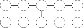
Figure 1: A simple cluster state. Note that each circle represents a single qubit in the cluster.

The basic element of the cluster-state model is the cluster state, an entangled network of qubits. An example of a cluster state is represented in Figure 1. Each circle represents a single qubit in the cluster. We may define the cluster state as being the result of the following two-part preparation procedure: first, prepare each qubit in the state $|+\rangle\equiv(|0\rangle+|1\rangle)/\sqrt{2}$, and then apply cphase gates between any two qubits joined by a line. Since the cphase gates commute with one another, it does not matter in what order they are applied. Note that this is merely a convenient way of defining the cluster state, and there is no requirement that it be prepared in this way.

Given the cluster state, a cluster-state computation is simply a procedure for measuring some subset of qubits in the cluster, using single-qubit measurements and feedforward of the measurement results to control the bases in which later qubits are measured. The output of the computation is the joint state of whatever qubits remain unmeasured at the end of the computation.

Figure 2: A two-qubit quantum circuit. Without loss of generality we may assume the computation starts with each qubit in the $|+\rangle\equiv(|0\rangle+|1\rangle)/\sqrt{2}$ state, since single-qubit gates can be prepended to the circuit if we wish to start in some other state. The two-qubit gate is a cphase gate. The boxes are single-qubit gates of the form $HZ_{\alpha}$, where $H$ and $Z_{\alpha}$ are as defined in Subsection II.2. Note that by composing three of these gates we can obtain an arbitrary single-qubit gate. Thus, gates of the form $HZ_{\alpha}$, together with cphase gates, are universal for quantum computation.

Remarkably, this procedure can be used to simulate an arbitrary quantum circuit. Indeed, the cluster state of Figure 1 was specifically chosen in order to simulate the circuit in Figure 2. In Figure 3 we illustrate visually how the cluster state of Figure 1 can be used to simulate the circuit in Figure 2. Each qubit in the quantum circuit is replaced by a horizontal line of qubits in the cluster state. Different horizontal qubits in the cluster represent the original qubit at different times, with the progress of time being from left to right. Each single-qubit gate $HZ_{\alpha}$ in the quantum circuit is replaced by a single qubit in the cluster state. cphase gates in the original circuit are simulated using a vertical “bridge” connecting the appropriate qubits. The cluster-state computation itself is carried out by performing a series of measurements in the time order and measurement bases indicated in the caption to Figure 3. The final output of the cluster-state computation $|\psi\rangle$ is related to the output of the quantum circuit $|\phi\rangle$ by $|\psi\rangle=\sigma|\phi\rangle$, where $\sigma$ is a product of Pauli matrices that is an easy-to-compute function of the measurement outcomes obtained during the cluster-state computation.

Although the example we have described involves a specific quantum circuit, general quantum circuits can be given a cluster-state simulation along similar lines. Note that we have not explicitly explained how the measurement feedforward procedure works, nor the precise function of measurement outcomes that determines the Pauli correction $\sigma$ at the end of the computation. These are explained in detail in Raussendorf and Briegel (2001); Nielsen (2003b); we also give an explicit description of the procedures used in Section IV.

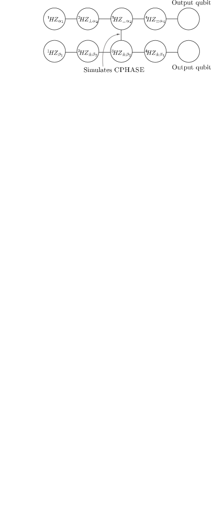
Figure 3: The cluster state of Figure 1, marked to indicate how it is used to simulate the different elements in the circuit of Figure 2. Note that the labeled qubits all have labels of the form “${}^{n}U$”, where $n$ is a positive integer, and $U$ is a unitary operation. The label $n$ indicates the time order; qubits with the same label can be measured in either order, or simultaneously. $U$ indicates that the qubit is measured by performing the unitary $U$ and then measuring in the computational basis. Equivalently, a single-qubit measurement in the basis $\{U^{\dagger}|0\rangle,U^{\dagger}|1\rangle\}$ is performed. Note that except for the first measurements, all measurements have $U$ of the form $HZ_{\pm\alpha}$; the $\pm$ indicates that the value of the sign depends upon the outcomes of earlier measurements. The output from the computation is at the unlabeled qubits, which are not measured.

One feature of our example quantum circuit, Figure 2, that deserves attention is the fact that it doesn’t involve any ancilla qubits. An important feature of many quantum circuits is that they involve the preparation and discarding of ancillas during the computation. This is especially true of circuits for quantum error-correction and fault-tolerant quantum computation, where the ancillas are used as a heat sink to remove excess entropy from the computer. Such ancilla preparations and removal are easily simulated in the cluster-state model. Figure 4 illustrates a simple quantum circuit involving an ancilla that is prepared and later discarded. Figure 5 illustrates how this preparation and discarding can be simulated within the cluster-state model.

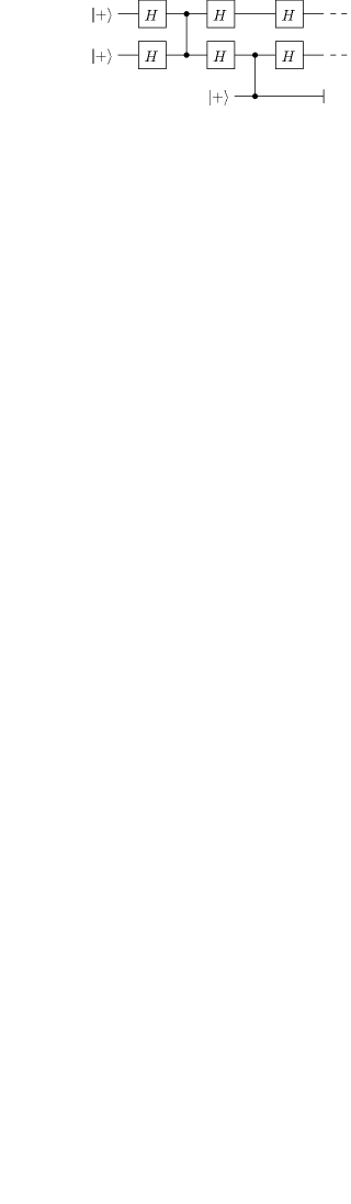
Figure 4: A simple quantum circuit in which an ancilla is prepared and later discarded.

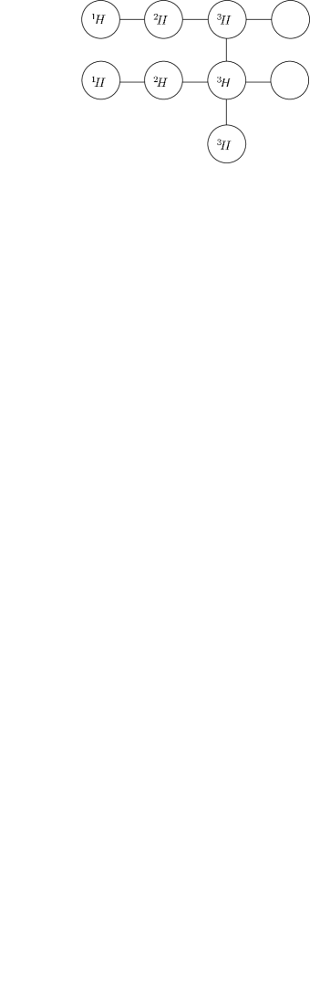
Figure 5: The cluster-state computation used to simulate the circuit in Figure 4.

The cluster states we have described so far have all been embedded in two dimensions. This is for convenience only. In practice, a more complicated topology for the cluster may be useful in some circumstances. This may be achieved either by embedding the cluster in a higher number of dimensions, or by nonlocal connections between different parts of the cluster. Fault-tolerant quantum circuits often involve two (or more) spatial dimensions, corresponding to a three-dimensional cluster-state computation. Note, however, that it does not follow that we require the use of all three spatial dimensions to do a cluster-state simulation of a two-dimensional quantum circuit. We will see below that it is only necessary to prepare a small part of the cluster at any given time, and this means that the cluster-state computation may be performed without requiring additional spatial dimensions beyond those used in the circuit being simulated.

Despite the different possible topologies of the cluster state, when convenient we shall continue to discuss cluster states as though they are embedded in two dimensions. This considerably simplifies discussion (and the figures), and the extensions to more complicated cluster topologies are in all cases obvious.

To facilitate later discussion of fault-tolerance we now introduce some additional nomenclature to describe cluster-state computations. We call a single vertical slice of qubits through the cluster a layer of the cluster. For example, in Figure 3 the two qubits with the label $4$ form a layer. A cluster-state simulation of a circuit thus consists of performing single-qubit measurements, layer by layer. We can think of a single layer in a cluster-state computation as similar to the instantaneous quantum state at some fixed time during a quantum circuit computation.

We call a single horizontal row of qubits through the cluster a level. So, for example, all the qubits on the top line of Figure 3 represent a level. We can think of a level as representing the evolution of a single qubit in a quantum circuit computation. We call a cluster-state computation involving only a single level a single-qubit cluster-state computation. The motivation for this nomenclature is that, as we have seen, such cluster-state computations are used to simulate single-qubit quantum circuits. Note that with this definition a single-qubit cluster-state computation may involve more than one physical qubit. A multi-qubit cluster-state computation is one that involves more than a single level of qubits.

Up until now, we have described a cluster-state computation as being composed of two steps: preparation of the cluster state, followed by an adaptive sequence of single-qubit measurements. However, it is also possible to implement cluster-state computations in alternative ways. The key observation is that we can delay preparation of some parts of the cluster until later, doing some of the measurements first. So, for example we could do a cluster-state computation via the following sequence of steps:

• Prepare layers one and two of the cluster, using $|+\rangle$ preparations and cphase gates.

• Perform the first layer of measurements.

• Prepare layer three, using $|+\rangle$ preparations and cphase gates to adjoin the third layer of qubits to the second layer.

• Perform the second layer of measurements.

• Keep alternating the steps of preparing an extra layer then measuring an extra layer, until the end of the computation.

We call this a one-buffered implementation of cluster state computation, since there is always a buffer of one layer between the layer of qubits being measured, and the most recently prepared layer of qubits. We call the set of qubits about to be measured the current layer, and the layer after that the next layer.

For fault-tolerance the one-buffered implementation of cluster-state computation has a great advantage over our original prescription in which the entire cluster is prepared first. The reason, as indicated in the introduction, is that if the entire cluster is prepared first, then qubits which are to be measured later in the computation will have undergone substantial degradation by the time they are measured, and this will unacceptably corrupt the output of the computation.

More generally, the one-buffered implementation illustrates the important point that a given cluster-state computation may have many different implementations, i.e., different methods for creating the cluster and performing the required single-qubit measurements. When proving fault-tolerant threshold theorems for cluster-state computation we will need to carefully specify the details of the implementation used. All the implementations used in this paper are variants on the one-buffered implementation.

III.2 Optical cluster-state quantum computing

Our description of cluster-state computation has been as an abstract model of quantum computation. As described in the introduction the cluster-state model also shows great promise as the basis for experimental implementations of quantum computation in optics Nielsen (2004). We now briefly describe the optical implementation of cluster-state computation, following Nielsen (2004), and some of the special challenges it poses for a proof of fault-tolerance.

The proposal of Nielsen (2004) is a modified version of the proposal of Knill, Laflamme and Milburn (KLM) Knill et al. (2001), and we now briefly review some of the basic elements of KLM, following the review in Nielsen (2004). KLM encodes a single qubit in two optical modes, $A$ and $B$, with logical qubit states $|0\rangle_{L}\equiv|01\rangle_{AB}$, and $|1\rangle_{L}\equiv|10\rangle_{AB}$. (Note that we are using the standard Bosonic occupation number representation on the right-hand side of these definitions, not the qubit notation, so that, for example, $|01\rangle_{AB}$ indicates zero photons in mode $A$, and one photon in mode $B$.) State preparation is done using single-photon sources, while measurements in the computational basis may be achieved using high-efficiency photodetectors. Such sources and detectors make heavy demands not entirely met by existing optical technology, although encouraging progress on both fronts has been reported recently. Arbitrary single-qubit operations are achieved using phase shifters and beamsplitters.

The main difficulty in KLM is achieving near-deterministic entangling interactions between qubits. KLM use the idea of gate teleportation Gottesman and Chuang (1999); Nielsen and Chuang (1997) to produce a gate $CZ_{n^{2}/(n+1)^{2}}$ which with probability $n^{2}/(n+1)^{2}$ applies a cphase to two input qubits, where $n$ is any fixed positive integer. When the gate fails, the effect is to perform a measurement of those qubits in the computational basis. Increasing values of $n$ correspond to increasingly complicated teleportation circuits. For this reason, KLM combine these ideas with ideas from quantum error-correction in order to achieve a near-deterministic cphase gate, and thus complete the set required for universal quantum computation.

An important property of the gate $CZ_{n^{2}/(n+1)^{2}}$ is that in the ideal case of perfect implementation, we know when the gate succeeds. In particular, in KLM’s implementation procedure, success of the gate is indicated by certain photodetectors going “click”, while failure is indicated by different photodetection outcomes. We call such gates postselected gates to indicate that whether the gate has succeeded is known, and can be fed forward to later parts of the computation.

The advantage of the optical cluster-state proposal of Nielsen (2004) is that it only makes use of the $CZ_{1/4}$ and $CZ_{4/9}$ gates, both of which use relatively simple configurations of optical elements, and avoids the use of error-correction in achieving a near-deterministic cphase gate. This results in a greatly simplified proposal for quantum computation.

A key observation used in the optical cluster-state proposal is an interesting general property of cluster states. Suppose we measure one of the cluster qubits in the computational basis, with outcome $m$. Then it can be shown that the posterior state is just a cluster state with that node deleted, up to a local $Z^{m}$ operation applied to each qubit neighbouring the deleted qubit. These are known local unitaries, whose effect may be compensated in subsequent operations, so we may effectively regard such a computational basis measurement as simply removing the qubit from the cluster.

This is a useful observation because when the $CZ_{n^{2}/(n+1)^{2}}$ gate fails, it effects a measurement in the computational basis. Thus, if one attempts to add qubits to a cluster using a $CZ_{n^{2}/(n+1)^{2}}$ gate, failure of the gate merely results in a single qubit being removed from the cluster, rather than the entire cluster being destroyed. Nielsen (2004) shows that by combining this observation with a random walk technique, it is possible to efficiently build up an arbitrary cluster state using either $CZ_{4/9}$ or $CZ_{1/4}$ gates. Once this is done, all the other operations in the cluster-state model can be done following KLM’s prescription.

IV Fault-tolerance with deterministic $CPHASE$ gates

In this section we prove a threshold theorem for noisy cluster-state quantum computation. This theorem is applicable to situations in which the cluster can be extended during the computation using cphase gates that are noisy, but operate deterministically. In the next section we extend the theorem to some situations where the cphase gates operate non-deterministically, as is the case for optical cluster-state computation.

Rather than attempt to invent fault-tolerant methods for cluster-state computation from scratch, it is natural to build off the existing and rather extensive body of literature on fault-tolerant quantum circuits. As described in the introduction, our strategy is to consider a cluster-state computation that simulates a fault-tolerant quantum circuit, and then ask if the simulated fault-tolerant capabilities are able to correct noise in the cluster-state implementation.

We therefore begin with a quantum circuit $\mathcal{Q}$ and, instead of directly translating it into the cluster-state model, first encode $\mathcal{Q}$ as a fault-tolerant circuit $\mathcal{F_{Q}}$ in the canonical form of Theorem 4. Recall that a canonical fault-tolerant circuit uses only preparations of qubits in the state $|+\rangle$, single-qubit gates of the form $HZ_{\alpha}$, and the two-qubit gate $\left(H\otimes H\right)$cphase. Using the prescription described in Section III it is a simple matter to translate $\mathcal{F_{Q}}$ into a cluster-state computation, which we denote $\mathcal{C}$.

Suppose now that $\mathcal{C}^{\prime}$ is a noisy one-buffered implementation of $\mathcal{C}$. Is $\mathcal{C}^{\prime}$ equivalent to some noisy implementation $\mathcal{F_{Q}}^{\prime}$ of $\mathcal{F_{Q}}$? We will show in this section that this is indeed the case, and moreover that the noise is of a type and strength that is correctable by the fault-tolerance built into $\mathcal{F_{Q}}$. The noisy cluster-state computation $\mathcal{C}^{\prime}$ is therefore a fault-tolerant simulation of the original quantum circuit $\mathcal{Q}$. It is worth noting that this noise correspondence holds for any quantum circuit and its corresponding one-buffered implementation; we don’t use any special properties of ${\cal F_{Q}}$ in proving the noise correspondence.

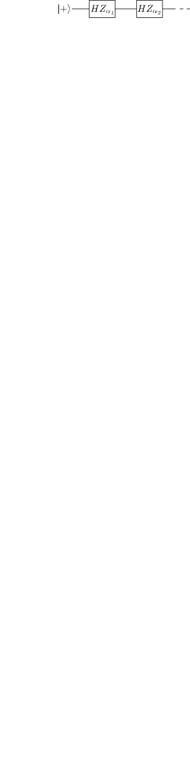
Figure 6: A single-qubit circuit containing only operations from the canonical set.

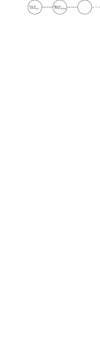
Figure 7: A cluster-state computation implementing the single-qubit circuit shown in Figure 6. We will show that the noise in this single-qubit cluster-state computation can be mapped onto equivalent noise in the corresponding quantum circuit.

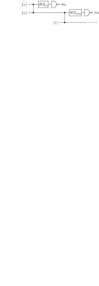
Figure 8: The literal circuit for the one-buffered implementation of the cluster-state computation in Figure 7.

A key construction used in establishing this noise correspondence is what we call the literal quantum circuit, $\mathcal{L}$. The literal circuit is a quantum circuit depiction of the operations performed during a one-buffered implementation of a cluster-state computation. It is a literal translation of the one-buffered implementation, and should not be confused with the quantum circuit $\mathcal{F_{Q}}$ being simulated. As an example, consider the single-qubit quantum circuit depicted in Figure 6. The corresponding cluster-state computation is depicted in Figure 7, and the literal circuit showing the one-buffered implementation is shown in Figure 8. Note that although $3$ qubits appear in the literal circuit, the quantum circuit being simulated is a single-qubit computation.

The literal circuit $\mathcal{L}$ offers a convenient means for describing the effects of noise in $\mathcal{C}^{\prime}$, and for this reason we have gone to some trouble in Figure 8 to depict the correct time-ordering of events. We have, for example, offset the preparation of the final $|+\rangle$ state, since it is not actually prepared until later in the one-buffered implementation, and preparation at an earlier time would result in considerably more noise affecting the qubit.

The noise in $\mathcal{C}^{\prime}$ is quantified by the error strength $\Delta_{Q:E}$ of the operations appearing in the literal circuit. The key result of this section is that if the worst-case noise strength in $\mathcal{C}^{\prime}$ is $\eta$, then the corresponding noise in the quantum circuit $\mathcal{F_{Q}}^{\prime}$ satisfies the locality assumption and has strength at most $c\eta$, for some constant $c$. Provided $c\eta\leq\eta_{\mathrm{th}}$ we conclude that the distribution $p^{\prime}$ that results when we measure the output of the cluster-state computation satisfies $\|p-p^{\prime}\|_{1}\leq\epsilon$, where $p$ is the distribution output from the noise-free computation.

The section contains three parts. Subsection IV.1 introduces our noise model for cluster-state computation. Subsection IV.2 proves the noise correspondence described above for the simplest case when the quantum circuit $\mathcal{F_{Q}}$ and the corresponding cluster-state computation $\mathcal{C}$ are single-qubit computations. All the ideas introduced in this subsection are then extended to the case of a multi-qubit $\mathcal{F_{Q}}$ and $\mathcal{C}$ in Subsection IV.3.

IV.1 Noise model for a one-buffered cluster-state computation

The noise model appropriate to a cluster-state computation depends critically upon the implementation procedure used to perform the computation. The results in this section are based on the one-buffered implementation procedure, as described in Section III. Recall that in a one-buffered implementation the only qubits available in the cluster at any given time are the qubits in the current layer, and the next layer. The computation is performed by repeatedly performing the following two steps: (1) making all the necessary measurements on the current layer; and (2) using cphase gates to add an extra layer of qubits into the cluster. The only variation in this procedure comes at the very beginning of the computation, where we need to create two whole layers of cluster-state qubits, and at the end, where we don’t need to add an extra layer into the cluster.

As in the fault-tolerance results for quantum circuits, our results do not allow for completely arbitrary types of noise. Instead, we make some physically plausible assumptions about the nature of noise in the one-buffered implementation. The noise model we adopt allows for the following types of noise:

1. Noise in unitary dynamics: We model this in a manner similar to the noise model for quantum circuits described in Subsection II.2. Each qubit has its own environment, and we assume that non-interacting qubits have non-interacting environments, but make no other assumptions about the noise. Indeed, we can use an even more general noise model, in which qubits at the same level in the cluster state are assumed to share a common environment, and all we assume is that non-interacting levels have non-interacting environments.

2. Noise in quantum memory: Quantum memory is simply the (unitary) identity operation, and we model a noisy quantum memory step as we would any other noisy unitary operation. Note that this type of noise affects all qubits other than the current layer during a round of measurements.

3. Noise in preparation of the $|+\rangle$ state: We model this is as perfect preparation of $|+\rangle$, followed by a noisy quantum memory step.

4. Noise in measurements in the computational basis: We model this as a noisy quantum memory step, followed by a perfect measurement in the computational basis.

We quantify the overall strength of noise in a one-buffered cluster-state computation by the worst-case error strength in any of the unitary operations, including the noisy quantum memory steps in preparation and measurement.

IV.2 Noise correspondence for single-qubit computations

In this section we consider the simplest case of a single-qubit circuit $\mathcal{F_{Q}}$ made up of gates $HZ_{\alpha_{j}}$, as shown in Figure 6. A cluster-state computation $\mathcal{C}$ simulating $\mathcal{F_{Q}}$ is shown in Figure 7. The establishment of the noise correspondence is a five-step process. To help orient the reader, we now outline these steps. Note that the meaning of these steps may not be completely clear upon a first read, but hopefully will ease comprehension of later parts of the paper.

1. We begin with the literal circuit $\mathcal{L}$ depicting a one-buffered implementation of $\mathcal{C}$. Such a circuit is shown in Figure 8.

2. The literal circuit of Figure 8 does not explicitly contain the classical feedforward and control that is performed during the cluster-state computation. Without taking these into account, it is not possible to understand the effects of noise on the computation. Thus, we expand $\mathcal{L}$ to explicitly include the classical feedforward and control.

3. We use a series of circuit identities to transform the literal circuit $\mathcal{L}$ into an equivalent circuit that contains “block” operations $B_{\alpha_{j}}$, each of which correspond directly to the action of some gate $HZ_{\alpha_{j}}$ in $\mathcal{F_{Q}}$. Looking ahead, the block form equivalent to a perfectly implemented $\mathcal{L}$ is depicted in Figure 17, with the $B_{\alpha_{j}}$ shown in Figure 18.

4. The threshold theorem of Terhal and Burkard involves only unitary operations. Thus, the next step is to replace the classical elements of the blocks $B_{\alpha_{j}}$ with unitary quantum equivalents to obtain a unitary operation $QB_{\alpha_{j}}$. Looking ahead, the correspondence with the $HZ_{\alpha_{j}}$ of $\mathcal{F_{Q}}$ is explicitly shown in Proposition 5. The circuit equivalent to the literal circuit but containing unitary blocks is shown in Figure 22, with the $QB_{\alpha_{j}}$ defined in Figure 20.

5. It can now be shown that noise in $\mathcal{C}$ is equivalent to noise within the unitary blocks $QB_{\alpha_{j}}$. Using Proposition 5 and the first unitary extension theorem, Theorem 1, we show that noise of strength $\eta$ in $QB_{\alpha_{j}}$ corresponds to noise of strength at most $c\eta$ in $HZ_{\alpha_{j}}$, for some appropriate constant $c$.

Our first task in this subsection, then, is to explicitly insert the classical control and feedforward operations into the literal circuit $\mathcal{L}$ of Figure 8, and to arrange that circuit into an appropriate block form. We begin by inserting perfect swap gates into $\mathcal{L}$ to obtain a more compact (but equivalent) circuit which is shown in Figure 9. We may assume that these swap gates operate perfectly as they are merely a mathematical convenience. The remaining operations in Figure 9, however, are real operations and will be subject to noise. When we need to emphasize that a circuit contains a mix of both real and perfect operations we will refer to it as an imperfect circuit, as distinct from a noisy circuit where all operations are subject to noise.

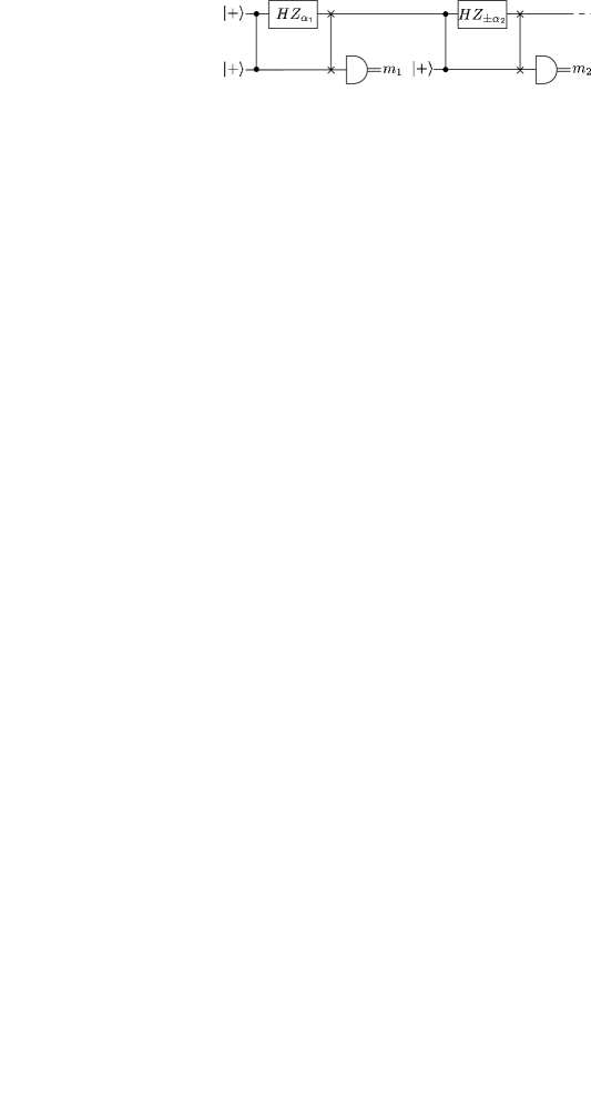
Figure 9: A circuit with the same output as that of Figure 8. The new two-qubit gates that have been inserted are swap gates.

There are two classical aspects of the cluster-state computation that we have not yet explicitly included in the literal circuit. These are the Pauli corrections introduced by the measurement, and the classical feedforward of measurement results to account for these corrections. As an example, consider the first measurement in Figure 8. This introduces a correction $X^{m_{1}}$ to the state of the qubit immediately below and consequently the second measurement is performed in the basis $HZ_{\pm\alpha_{2}}$ according to whether $m_{1}$ is $0$ or $1$. In general, the Pauli correction is given by $X^{x}Z^{z}$ where $x$ and $z$ are classical variables. Initially $x$ and $z$ are both zero, and they are updated after each measurement by the rule

$$x^{\prime} = z+m\,\,(\mathrm{mod}\,\,2)$$ (21)

$$z^{\prime} = x\,\,(\mathrm{mod}\,\,2),$$ (22)

where $m=0,1$ is the measurement outcome. Subsequent measurement is performed in the basis $HZ_{\pm\alpha_{j}}$, with the choice determined by whether $x$ is $0$ or $1$.

The two classical variables $x$ and $z$ have been introduced into the circuit in Figure 10. The $E$rror $U$pdate operation $EU$ updates $x$ and $z$ using Equations (21) and (22), and the variable $x$ is used to control the rotations $HZ_{\pm\alpha_{j}}$. An explicit definition of $EU$ is shown in Figure 11. The circuit of Figure 10 can be made more compact by introducing the notation of Figure 12 for the classical feedforward. The resulting circuit is shown in Figure 13.

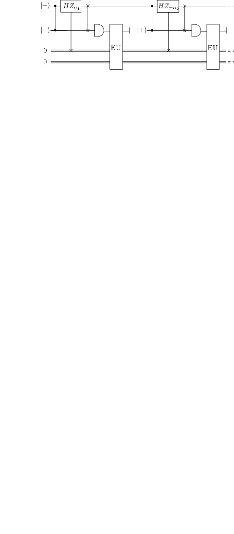
Figure 10: A circuit with the same output as Figure 9, but with the classical controls explicitly drawn in. Note that $x$ is the top bit, while $z$ is the lower bit. The new circuit notation involving the $HZ_{\alpha_{1}}$ and $HZ_{\alpha_{2}}$ operations indicates how the classical variable $x$ is used to control the measurement basis. A value of $x=0$ means that $HZ_{\alpha}$ is applied, while a value of $x=1$ means that $HZ_{-\alpha}$ is applied. Note that in the case of $HZ_{\alpha_{1}}$, we always have $x=0$, and so $HZ_{\alpha_{1}}$ is applied, as expected.

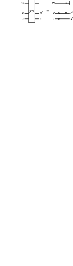
Figure 11: The classical error update circuit, following Equations (21) and (22).

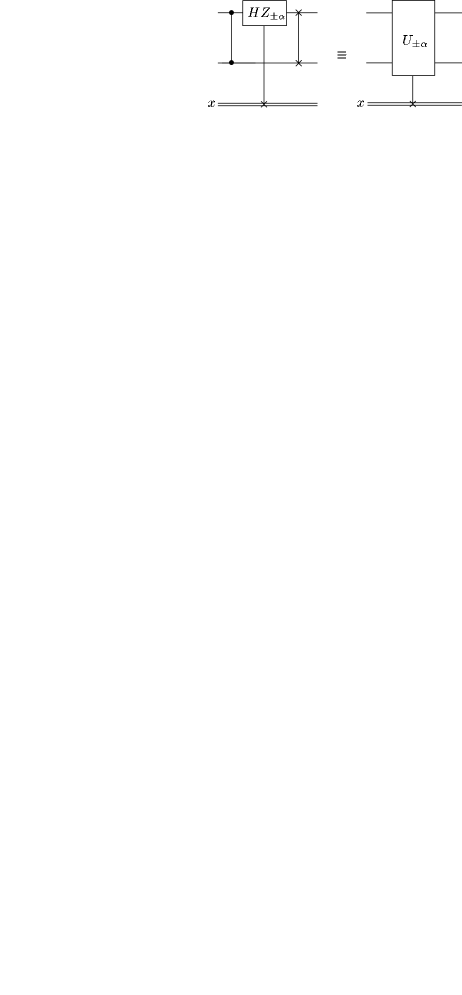
Figure 12: A definition to make other circuits more compact.

We have made several modifications to the literal circuit $\mathcal{L}$, but the output of the imperfect circuit shown in Figure 13 is still equivalent to the output of the noisy literal circuit in Figure 8. To complete the construction of the blocks $B_{\alpha_{j}}$ referred to earlier in Step $3$, we introduce some additional circuit identities whose effect is to compensate for the corrections $X^{x}Z^{z}$. This will enable us to make exact the correspondence with the gates $HZ_{\alpha_{j}}$ in the quantum circuit $\mathcal{F_{Q}}$.

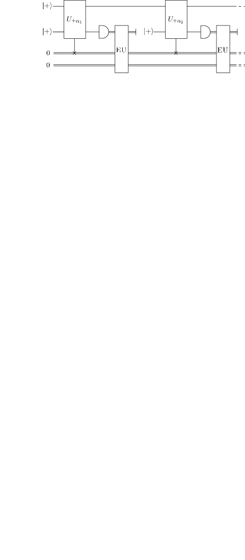
Figure 13: The output of Figure 8 is the same as the output of this imperfect circuit.

First, at the beginning of the first block in Figure 13, we prepend the gates illustrated in Figure 14. These are perfect gates, and can be prepended without changing the output of Figure 13, since the initial values of $x$ and $z$ are both zero.

Figure 14: The output of Figure 13 is unchanged if these perfect gates are prepended at the beginning of the computation.

Second, we modify the very final block in Figure 13 (which is not explicitly shown), appending operations inverse to those in Figure 14, as illustrated in Figure 15. The reason we may do this is as follows. If all the operations in the cluster-state computation are implemented perfectly, then at the end of the computation the qubit would be in the state $X^{x}Z^{z}|\psi\rangle$, where $|\psi\rangle$ is the output from the corresponding perfect quantum circuit computation. If we then measure this state in the computational basis, we can compensate for the error operator $X^{x}Z^{z}$ by appropriate post-processing of the measurement result, i.e., by adding $x$ to the outcome of the measurement, modulo two. This process of compensating the measurement results is, however, equivalent to appending the perfect gates illustrated in Figure 15, and dropping the process of compensation.

Figure 15: The effective output of Figure 13 is unchanged if these perfect gates are appended at the end of the computation.

Our third and final modification is to insert the perfect gates of Figure 16 between each pair of the repeating blocks in Figure 13. Another way of stating this is that we insert the circuit of Figure 15 at the end of every block in the computation, except the last block, where it has already been inserted, and insert the circuit of Figure 14 at the beginning of every block in the computation, except the first, where it has already been inserted. This insertion does not modify the output of the circuit, since, as is apparent from Figure 16, these gates cancel one another out.

Figure 16: We insert these perfect gates between each pair of blocks in Figure 13.

With these modifications, we see that the output of the noisy cluster-state computation in Figure 8 is equivalent to the output of the imperfect circuit illustrated in Figure 17, where the operation $B_{\alpha}$ is defined in Figure 18.

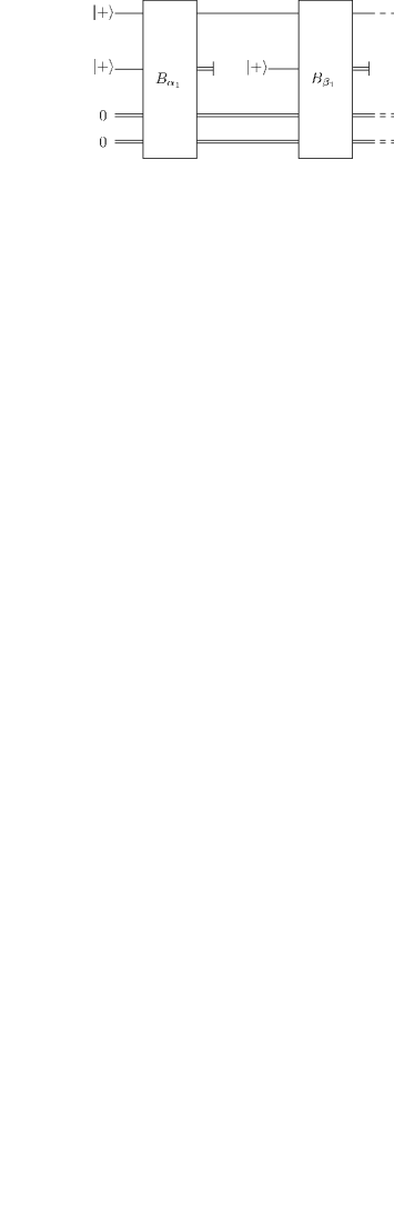
Figure 17: The output of this imperfect circuit is the same as the output of the noisy cluster-state computation in Figure 8.

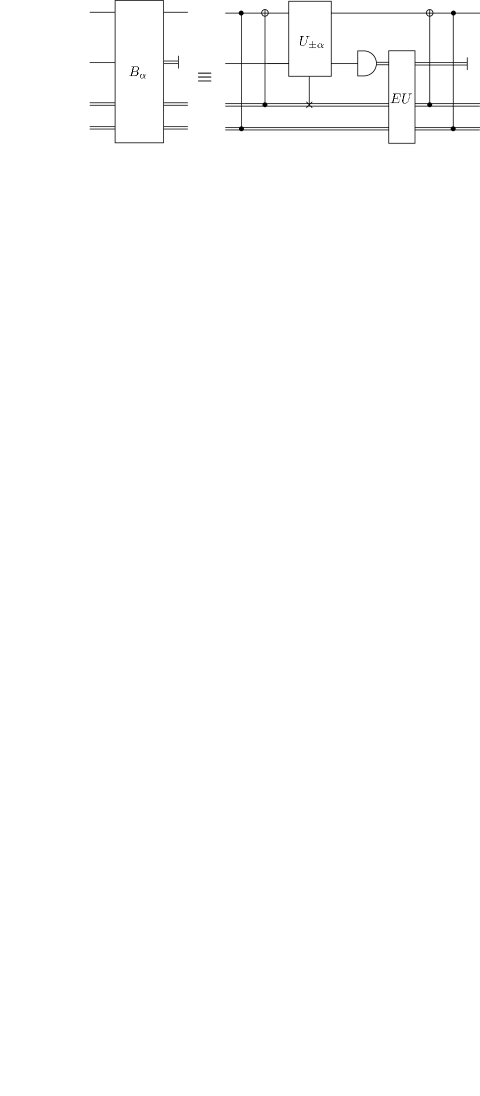
Figure 18: The definition of the operation $B_{\alpha}$ used as the basis for the repeating blocks in Figure 17.

This completes the construction of the repeating blocks $B_{\alpha}$. The circuit shown in Figure 17 allows us a fiction of identifying the topmost qubit $Q$ as a persistent data qubit carrying the information in a cluster-state computation. We will see that $B_{\alpha}$ effectively performs single-qubit gates on $Q$. To see how each $B_{\alpha}$ corresponds to a gate in the quantum circuit $\mathcal{F_{Q}}$ consider the circuit identity shown in Figure 19. This identity shows that a perfect implementation of $B_{\alpha}$ is equivalent (up to a known global phase factor) to the effect of applying a perfect $HZ_{\alpha}$ gate to the first qubit, initially in the state $|\psi\rangle$. Intuitively, then, we would expect that the result of the actual imperfections in $B_{\alpha}$ would be to effect an imperfect $HZ_{\alpha}$ gate. That is, we obtain a way of translating our noisy cluster-state computation into an equivalent noisy quantum circuit computation.

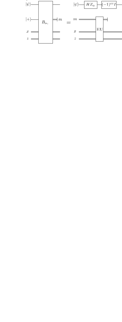
Figure 19: The output of the circuit on the left is identical to the output of the circuit on the right. For this identity we assume that all operations in both circuits are done perfectly — there is no noise.

We have introduced the identity of Figure 19 for motivational purposes only; we omit a proof, as we prove a stronger result later. Interested readers may wish to confirm this identity by hand. What we do now is find a way of showing quantitatively that noise in the imperfect operation $B_{\alpha}$ may be mapped to noise in the quantum circuit $\mathcal{F_{Q}}$.

The next step in our proof, Step $4$, is to replace the classical elements in $B_{\alpha_{j}}$ with unitary quantum equivalents to obtain fully unitary blocks, which we denote $QB_{\alpha_{j}}$. The reason for doing so will become clear in the final step of the proof, where we use the first unitary extension theorem, Theorem 1, to compare an imperfect $QB_{\alpha_{j}}$ to a noisy $HZ_{\alpha_{j}}$.

The classical elements of $B_{\alpha_{j}}$ are the classical variables $x,z$; the error update operation $EU$; and the classical controlled $U_{\pm\alpha}$. These have all been replaced by quantum equivalents to define $QB_{\alpha_{j}}$ in Figure 20. The quantum error update operation $QEU$ is defined in Figure 21, and $U_{\pm\alpha}$ is defined as before but with a quantum control. The bits carrying $x$ and $z$ have been replaced by qubits which we label $X$ and $Z$. We therefore assume that operations performed on these qubits are noiseless, including the operations in $QEU$.

The output of the noisy literal circuit $\mathcal{L}$ is thus equivalent to the output from the imperfect circuit in block unitary form shown in Figure 22. The qubit labeled $Q$ is persistent, and we can see that the cluster-state computation can be thought of as the successive application of unitaries $QB_{\alpha_{j}}$. These unitaries require three ancilla to perform an operation on $Q$, but the following proposition shows that, when all operations are done perfectly, the effect of each $QB_{\alpha_{j}}$ on $Q$ is identical to that of $HZ_{\alpha_{j}}$.

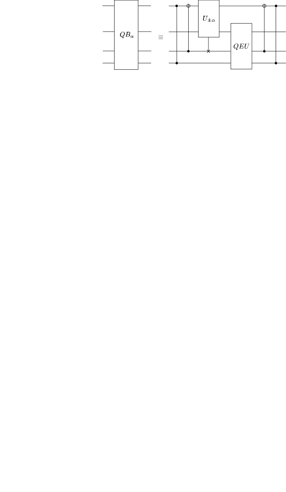
Figure 20: The definition of the operation $QB_{\alpha}$.

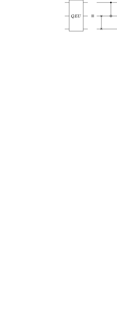
Figure 21: The definition of the quantum error update operation, $QEU$.

Figure 22: The output at $Q$ in this imperfect circuit is identical to the output of the imperfect circuit of Figure 17, and thus is equivalent to the output of the noisy cluster-state computation of Figure 8.

Proposition 5

The circuit identity of Figure 23 holds, where both circuits are assumed to be perfect. All inputs are assumed to be arbitrary, except the fixed $|+\rangle$ input, as shown.

The proof of the circuit identity of Figure 23 is straightforward, but somewhat technical. The details are sketched in Appendix B.

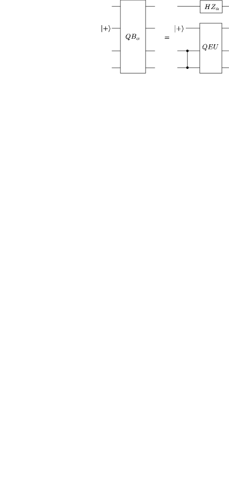
Figure 23: The circuit identity of Proposition 5. This is a perfect circuit identity, i.e., all elements in both circuits are assumed to be performed without any noise.

The final step in establishing the noise correspondence for single-qubit computation is to use Proposition 5 and the first unitary extension theorem, Theorem 1, to argue that an imperfect implementation of $QB_{\alpha_{j}}$ is equivalent to a noisy operation $HZ_{\alpha_{j}}$. Following the noise model of Subsection IV.1, let $E$ be the environment responsible for the noisy operations in the imperfect implementation of $QB_{\alpha_{j}}$. We denote this imperfect operation by $QB_{\alpha_{j}}^{\prime}$, a unitary acting on $QM_{j}XZE$. By assuming that the same environment $E$ is reused by all the imperfect operations $QB_{\alpha_{j}}^{\prime}$ we make the most pessimistic assumption we can possibly make about noise in the cluster-state computation. In the more general multi-qubit situation this assumption will correspond to assuming that all the qubits in the same level of the cluster share the same environment.

Now, suppose $\eta$ is the maximal error strength in any of the noisy operations making up the imperfect $QB_{\alpha_{j}}$. That is, $\eta$ quantifies the strength of the noise in the cluster-state computation. Let $c$ be the number of noisy operations in the imperfect $QB_{\alpha_{j}}$. Then the chaining property, Proposition 1, implies that

$$\Delta_{QM_{j}XZ:E}(QB_{\alpha_{j}},QB_{\alpha_{j}}^{\prime})\leq c\eta,$$ (23)

where $QB_{\alpha_{j}}$ is the perfect $QB_{\alpha_{j}}$ operation. Note our convention that in algebraic expressions we always use $QB_{\alpha_{j}}^{\prime}$ to refer to the imperfect operation, while in the text we sometimes use $QB_{\alpha_{j}}$ to refer to the imperfect operation, provided the context is clear. It follows that there exists a unitary operation $U_{E}$ on $E$ such that

$$\|QB_{\alpha_{j}}^{\prime}-QB_{\alpha_{j}}\otimes U_{E}\|\leq c\eta.$$ (24)

(Note that $U_{E}$ may depend on $j$, but that dependence is not important in the argument that follows, and so is suppressed.)

So, if $QB_{\alpha_{j}}^{\prime}$ is the noisy implementation of $QB_{\alpha_{j}}$, can we show that this corresponds to a noisy implementation of $HZ_{\alpha_{j}}$? In Figure 22 we see that the qubit $M_{j}$ is always initially prepared in the state $|+\rangle$. This is an exact statement, since imperfect preparation of the state $|+\rangle$ is modeled as a perfect preparation, followed by a noisy quantum memory step that is absorbed into the imperfect operation $QB_{\alpha_{j}}$. Define $S_{j}$ to be the subspace of $QM_{j}XZE$ in which $M_{j}$ is in the state $|+\rangle$, and the other systems may be in an arbitrary state. Then define $U_{j}\equiv QB_{\alpha_{j}}\otimes U_{E}$ and $V_{j}\equiv QB_{\alpha_{j}}^{\prime}$. Define $\tilde{U}_{j}$ as shown in Figure 24. By Proposition 5 we see that $U_{j}\big{|}_{S_{j}}=\tilde{U}_{j}\big{|}_{S_{j}}$ and so we can apply the first unitary extension theorem, Theorem 1, to conclude that there exists a unitary extension $\tilde{V}_{j}$ of $V_{j}|_{S_{j}}$ such that

$$\|\tilde{V}_{j}-\tilde{U}_{j}\| \leq \|V_{j}-U_{j}\|$$ (25)

$$= \|QB_{\alpha_{j}}^{\prime}-QB_{\alpha_{j}}\otimes U_{E}\|$$ (26)

$$\leq c\eta.$$ (27)

Applying Proposition 2 we see that

$$\Delta_{Q:M_{j}XZE}(HZ_{\alpha_{j}},\tilde{V}_{j})\leq c\eta.$$ (28)

Next, define $M=M_{1}\otimes M_{2}\otimes\ldots$ to be the combination of all the systems $M_{j}$. Applying Proposition 3 and Equation (28) we see that

$$\Delta_{Q:E^{\prime}}(HZ_{\alpha_{j}},\tilde{V}_{j})\leq c\eta,$$ (29)

where $E^{\prime}\equiv MXYE$ is the effective environment for the qubit $Q$, and we have extended $\tilde{V}_{j}$ to act in the natural way on $E^{\prime}$, i.e., $\tilde{V}_{j}$ acts trivially on systems $M_{k}$ such that $k\neq j$. Because $\tilde{V}_{j}|_{S_{j}}=V_{j}|_{S_{j}}$ we see that the noisy implementation $V_{j}=QB^{\prime}_{\alpha_{j}}$ of $QB_{\alpha_{j}}$ is exactly equivalent to a noisy implementation $\tilde{V}_{j}$ of $HZ_{\alpha_{j}}$ of strength at most $c\eta$.

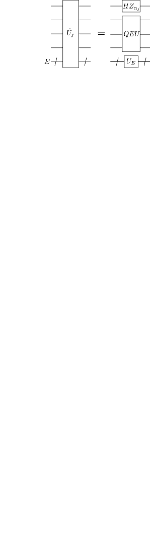
Figure 24: The definition of the operation $\tilde{U}_{j}$ The environment $E$ is shown at the bottom, where the wire with a slash through it indicates an arbitrary quantum system.

To conclude, we have shown that if the one-buffered cluster-state computation depicted in Figure 8 is implemented with noise of strength at most $\eta$ in each operation, then the output of that computation is equivalent to the output of the noisy quantum circuit in Figure 25, where each operation is performed with noise of strength at most $c\eta$. As we have described it, $c$ is the number of noisy operations in the imperfect operation $QB_{\alpha}$, i.e., $c\approx 10^{1}$. In actual implementations it would be possible to directly evaluate the total strength of the noise in the imperfect operation $QB_{\alpha}$, resulting in a more accurate (and better, from the point of view of the threshold) value for $c$.

A interesting feature of our argument is that even if the various physical operations involve only Markovian noise, the corresponding effective noise in the implementation of $HZ_{\alpha_{j}}$ is inherently non-Markovian. The reason is that the qubits $X$ and $Z$ associated with the classical variables $x$ and $z$ are part of the effective environment of $Q$ at every stage of the computation, due to the necessity of feeding forward the measurement results. This is the reason we need to use the non-Markovian threshold result of Terhal and Burkard Terhal and Burkard (2004).

Figure 25: This noisy circuit is equivalent to the noisy one-buffered cluster-state computation of Figure 8.

IV.3 Noise correspondence for multi-qubit computations

Figure 26: An illustrative two-qubit quantum circuit $\mathcal{F_{Q}}$ using canonical fault-tolerant gates.

Figure 27: A noisy two-qubit cluster-state computation.

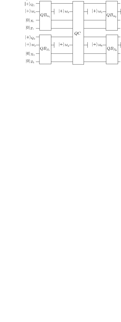
Figure 28: The output of this imperfect circuit is equivalent to the output of the noisy two-qubit cluster-state computation in Figure 27. The operations $QB_{\alpha_{j}},QB_{\beta_{j}}$ are as defined in the previous subsection, while $QC$ is defined in Figure 29.

In this subsection we extend the ideas of the previous subsection, explaining how noise in a multi-qubit one-buffered cluster-state quantum computation may be mapped to equivalent noise in the corresponding quantum circuit. The ideas used to do this are the same as were used in the proof for single-qubit cluster-state computations. As a result, we merely sketch out how the proof goes for a specific example, with the general proof following similar lines.

The noise correspondence is established via the same process followed in Subsection IV.2. We begin with a multi-qubit quantum circuit like the circuit $\mathcal{F_{Q}}$ shown in Figure 26. The cluster-state computation $\mathcal{C}$ simulating this circuit is shown in Figure 27. As before, we construct a literal circuit and rearrange it into the block form where each block is identifiable with a gate in the quantum circuit $\mathcal{F_{Q}}$. We have omitted the details of this rearrangement, and presented the final block form equivalent to the literal circuit in Figure 28. The blocks $QB_{\alpha_{j}},QB_{\beta_{j}}$ correspond to the single-qubit gates $HZ_{\alpha_{j}},HZ_{\beta_{j}}$ in $\mathcal{F_{Q}}$, as in the previous subsection, and the effects of noise in these blocks has already been considered. The new element is the unitary block $QC$, which is shown in detail in Figure 29. The following proposition shows that a perfect implementation of $QC$ effects the operation $(H\otimes H)$cphase on the qubits $Q_{1}$ and $Q_{2}$.

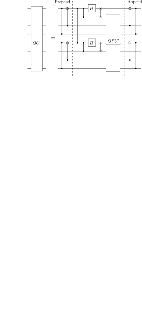
Figure 29: The definition of the imperfect operation $QC$ appearing in Figure 28. We have prepended and appended the same fictitious elements used in the single-qubit case in Figures 14 and 15. The gate $QEU^{\prime}$ is the two-qubit extension of the error update, and is shown in detail in Figure 30. The only noisy operations are the Hadamard gates, and the cphase gate between the first and the fifth qubits.

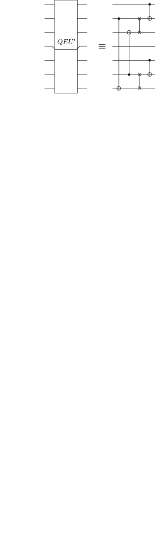
Figure 30: The definition of the two-qubit quantum error update operation analogous to that of Figure 21.

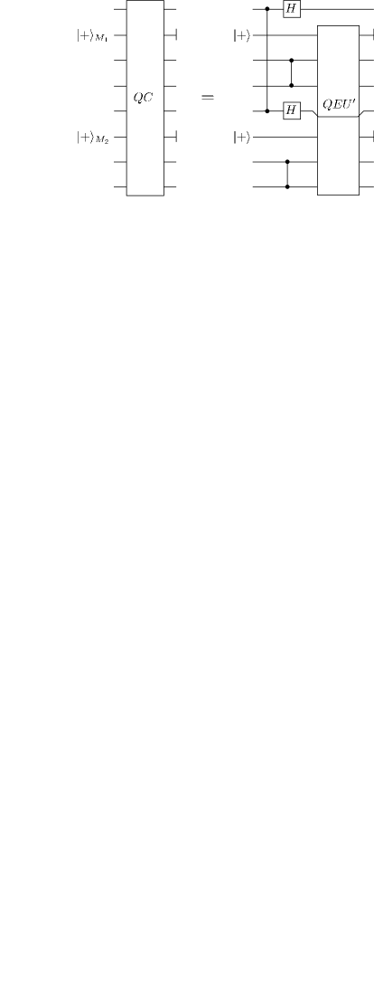
Figure 31: The circuit identity of Proposition 6. This is a perfect circuit identity, i.e., all elements in both circuits are assumed to be performed without any noise.

Proposition 6

The circuit identity of Figure 31 holds, where both circuits are assumed to be perfect.

Proof: The proof of this identity uses the same techniques as the proof of Proposition 5, and is omitted. The identity may easily be verified using any of the standard computer algebra packages.

QED

This proposition plays a similar role to that played by Proposition 5 in establishing the single-qubit noise correspondence. In this case the noise correspondence will again follow from the first unitary extension theorem.

Following the noise model of Subsection IV.1, we introduce environments $E_{1}$ and $E_{2}$ associated with the respective levels in the cluster-state computation of Figure 27. Under the locality assumption an imperfect $QB_{\alpha_{1}}$, for example, is thus represented as a unitary operator $QB_{\alpha_{1}}^{\prime}$ acting on $Q_{1}M_{1}X_{1}Z_{1}E_{1}$, which results in an effective environment for the corresponding $HZ_{\alpha_{1}}^{\prime}$ of $\tilde{E}_{1}=M_{1}X_{1}Z_{1}E_{1}$. As in the single-qubit case, the noise strength in the operations of the form $HZ_{\alpha}$ is at most $c\eta$, where $c\approx 10^{1}$ is a small constant, and $\eta$ is the noise strength in the operations used to implement the cluster-state computation.

An imperfect $QC$ is similarly represented as a unitary $QC^{\prime}$ which involves both the environments $E_{1}$ and $E_{2}$. Using the first unitary extension theorem we can show that this results in an effective environment $\tilde{E}_{12}=M_{3}X_{1}Z_{1}M_{4}X_{2}Z_{2}E_{1}E_{2}$ for the operation $(H\otimes H)$cphase in $\mathcal{F_{Q}}$. It follows that the noise strength in the $(H\otimes H)$cphase gate is at most $c^{\prime}\eta$, where $c^{\prime}$ is the total number of noisy operations in the imperfect operation $QC$, and again is of order $10^{1}$.

Summing up, suppose we perform a noisy one-buffered implementation of a cluster-state computation, satisfying the noise model described in Subsection IV.1, and with $\eta$ the maximal noise strength in any operation. Then we can show that this noisy computation is equivalent to performing the corresponding quantum circuit with noise satisfying the locality assumption, and of strength at most $c^{\prime\prime}\eta$, where $c^{\prime\prime}\approx 10^{1}$ is some constant. This completes the proof that quantum circuits may be simulated in a fault-tolerant fashion using a one-buffered cluster-state computation.

One remarkable feature of our proof is that it goes through unchanged even if we allow noise to occur in the classical computations and feedforward. It is easy to see that such noise simply causes an additional contribution to the strength of the noise in the corresponding quantum circuit, and thus a decrease in the effective threshold. This feature of the proof also carries over to the threshold theorem for optical cluster-state computation presented in the next section. Thus, our results show that not only can cluster-state computation be made resilient against the effects of unitary non-Markovian errors, it can even be made resilient against the effects of noise in the classical parts of the computation.

V Fault-tolerance with optical cluster states

In this section we explain how the ideas of Section IV can be extended to enable fault-tolerant simulation of quantum circuits using optical cluster states. The main challenge in proving this result is the non-deterministic nature of the entangling gates used in optical cluster-state computation. We show that this challenge can be met by using those non-deterministic gates to add additional pieces to the cluster in a near-deterministic fashion using what we call the dangling node implementation of optical cluster-state quantum computation. On those rare occasions when the addition to the cluster fails, one simply accepts failure and moves on, regarding the failure as a small amount of additional noise in a deterministic preparation of the cluster state. This allows us to apply the results of the Section IV to deduce a fault-tolerant threshold for optical cluster states.

Although we phrase our results in terms of optics, there may be other natural contexts in which our results apply. The crucial fact about the optical implementation that we use is the existence of a postselected non-deterministic cphase gate which, when it fails, effects a measurement in the computational basis. The threshold results we apply would apply equal well to other implementations which share this feature.

We begin our account in Subsection V.1 with an overview of the main elements of the proof. In particular, we explain the dangling node implementation in detail, and explain heuristically how noise in the dangling node implementation maps to noise in the quantum circuit model. Subsection V.2 discusses the noise model we use in our description of optical cluster-state computation. An important issue in this discussion is noise due to photon loss. As described in the introduction to this paper, the noise model used by Terhal and Burkard Terhal and Burkard (2004) does not explicitly allow for leakage errors, and thus noise due to photon loss is not directly addressed by our results. Nonetheless, we expect that with some straightforward modifications of the results in Terhal and Burkard (2004) it will be possible to cope with the problem of photon loss and other forms of leakage error in optical cluster-state computation. Subsection V.3 proves a rigorous threshold for what we call the two-at-a-time implementation of cluster-state computation. The two-at-a-time implementation makes use of deterministic cphase gates, and thus is not of immediate relevance for optical cluster-state computing. Its interest arises from the fact that it is intermediate in complexity between the one-buffered implementation studied in Section IV, and the full dangling node implementation of optical cluster-state computation. Analysing the two-at-a-time implementation thus provides a useful stepping stone on the way to understanding fault-tolerance in the dangling node implementation. Subsection V.4 introduces some useful nomenclature for describing postselected quantum gates, and proves a simple lemma about such gates. The threshold proof for optical cluster-state computation is completed in Subsection V.5, which explains how noise in the dangling node implementation may mapped to equivalent noise in the quantum circuit model.

V.1 Overview

The broad structure of the threshold proof for optics is similar to the proof for the deterministic one-buffered implementation discussed in Section IV. We take a quantum circuit that we wish to simulate, and turn it into a fault-tolerant quantum circuit, using the standard prescriptions for fault-tolerance. We then convert the fault-tolerant circuit into an equivalent cluster-state computation, and then specify in detail a specific implementation protocol for performing that computation. In this case that will be a dangling node implementation. We now describe how the dangling node implementation works. We will show in later subsections that noise in the dangling node implementation can be mapped onto equivalent noise in the original fault-tolerant quantum circuit. This enables us to deduce that the output of the noisy optical cluster-state computation is equivalent to the output of a noisy fault-tolerant quantum circuit computation, and thus to obtain a threshold result.

Figure 32: The microcluster used in the dangling node implementation of cluster-state computation. There are $k$ dangling nodes, in general; in this example, $k=3$.

We begin by describing the dangling node implementation for the simplest case of a single-qubit cluster-state computation. The basic idea is to to build the cluster up using small cluster states that we call microclusters. The basic microcluster is illustrated in Figure 32. It includes a single base node, on the left, and $k$ dangling nodes, on the right, where $k$ is some fixed constant.

Optically, we may prepare microclusters by sequentially performing $k$ non-deterministic cphase gates. These may be either the non-deterministic KLM cphase gate, or one of its more efficient (but still non-deterministic) modern descendants. Since $k$ is a constant, the expected number of operations required to form a microcluster is also constant. In practice, there are likely to be much more efficient means of preparing a microcluster than this procedure. However, for the purposes of this paper we shall not be concerned with optimizing the formation of the microcluster.

The dangling node implementation of a single-qubit cluster-state quantum computation works as follows. The first step is to prepare a single microcluster, as illustrated in Figure 32. This forms the basis from which a larger cluster state will gradually be grown by adjoining extra microclusters.

The second step of the dangling node implementation is to attempt to adjoin microclusters to each of the first $k-1$ dangling nodes of the first microcluster (i.e., all but the last of the dangling nodes), using non-deterministic cphase gates. If one of these attempts to adjoin should succeed, then we stop, and use computational basis measurements and single-qubit operations to ensure that we end up with the larger cluster state shown in Figure 33. To ensure that this works, it is critical that we use one of the special KLM non-deterministic cphase gates, which, as noted in Section III, have the property that failure of the gate results in a computational basis measurement, and removal of a qubit from the cluster. If all $k-1$ attempts to adjoin fail, then we simply accept the failure, and apply the appropriate single-qubit operation to end up with the larger cluster state shown in Figure 34. Note that if the non-deterministic KLM cphase gate fails with probability $p_{f}$, then the probability of successfully adjoining a microcluster, as in Figure 33, is $1-p_{f}^{k-1}$, while the probability of failing, as in Figure 34, is $p_{f}^{k-1}$. When the adjoinment succeeds, we effectively add two perfect extra layers of qubits to the cluster. Failure introduces a defect into the cluster, but we can ensure this occurs with small probability by choosing $k$ to be large.

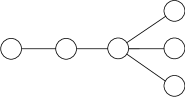
Figure 33: The cluster state which results after successfully adjoining a microcluster to the initial microcluster in Figure 32, deleting the extra nodes, and applying appropriate local operations.

Figure 34: The cluster state which results after failing $k-1$ times to adjoin a microcluster to the initial microcluster in Figure 32.

The third step of the dangling node implementation is to perform the first two layers of single-qubit measurements in the cluster-state computation. We then go back to the second step, effectively adding another two layers of qubits into the cluster, and so on, through the entire course of the computation. The only variation comes at the very end of the computation, where there is no need to adjoin a microcluster of the form in Figure 32, but instead we can add the simpler two-qubit microcluster illustrated in Figure 35.

Figure 35: The simpler two-qubit microcluster adjoined to the cluster state at the very end of a single-qubit cluster-state computation, in place of the microcluster in Figure 32.

We have seen how a single-qubit cluster-state computation may be performed in the dangling node implementation; what about multi-qubit cluster-state computations? The key is to introduce a third type of microcluster, illustrated in Figure 36. Once again, note that these microclusters may be prepared in constant expected time using non-deterministic cphase gates.

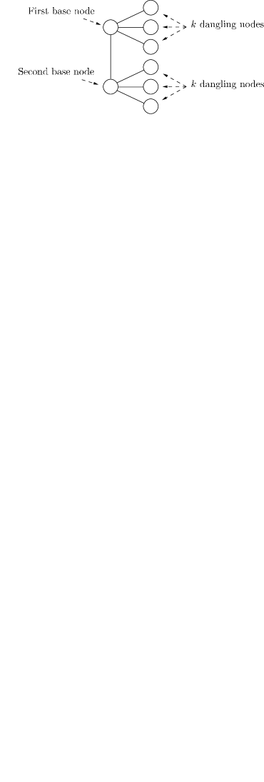
Figure 36: This microcluster is used in the dangling node implementation of multi-qubit cluster-state quantum computations.

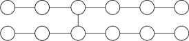
Figure 37: An example cluster-state computation. We have omitted explicit description of the measurements performed, since it is the formation of the cluster that we wish to concentrate on, rather than the details of the measurements.

Consider the cluster-state computation depicted in Figure 37. We may implement this computation as follows. The first step is to prepare the first two layers of the cluster. This may be done using the non-deterministic cphase gate in constant time, as described earlier.

The second step of the dangling node implementation is to add in two additional layers to the cluster. This is done in a similar fashion to the adjoinment of a microcluster in the single-qubit case. In this case, success requires that we adjoin the microcluster in Figure 36 to two different dangling nodes, one on the top level of the computation in Figure 37, the other to the bottom level. Success in adjoinment at both levels results in the cluster of Figure 38 being prepared. A simple calculation shows that this occurs with probability $1-2p_{f}^{k-1}+p_{f}^{2k-2}$, which approaches $1$ rapidly as $k$ becomes large. If, on the other hand, either adjoinment should fail, we simply declare failure overall, resulting in the cluster of Figure 39 being prepared. Note that if one part of the microcluster is successfully adjoined, but the other part fails, then it may be necessary to delete some nodes of the cluster using computational basis measurements and local $Z$ operations in order to obtain the cluster of Figure 39.

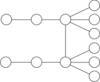
Figure 38: The cluster after successfully adding the microcluster of Figure 36.

Figure 39: The cluster after failing to add the microcluster of Figure 36.

The third step in the dangling node implementation of the computation in Figure 37 is to perform the first two layers of single-qubit measurements. The fourth step is to add in the final two layers of the cluster, which is done using the same procedure as for single-qubit computations. The fifth and final step of the implementation is to do the final four layers of single-qubit measurements in the standard way.

The generalization of the dangling node implementation to arbitrary multi-qubit cluster-state computations follows the same lines, alternating attempts to adjoin microclusters with two layers of single-qubit measurements. Each successful adjoinment of a microcluster adds two perfect extra layers to one or more levels of the cluster, while failure to adjoin correctly introduces a defect into the cluster, but occurs with probability $2p_{f}^{k-1}-p_{f}^{2k-2}$.

How does noise in the dangling node implementation map to noise in the quantum circuit model? A heuristic argument is as follows. Roughly speaking, each gate in the original circuit is simulated by adjoining a microcluster and performing some single-qubit measurements. Adjoining a microcluster involves up to $c_{1}k^{2}$ physical operations, where $c_{1}$ is some positive constant in the range $10^{0}$-$10^{2}$. If each operation is performed with error strength $\eta$, then the total associated noise is at most $c_{1}k^{2}\eta$. There is also an intrinsic failure probability, due to the non-determinism of the gates, which causes defects in the cluster. This probability is bounded by $2p_{f}^{k-1}$. Finally, the noise contribution due to the single-qubit measurements scales as $c_{2}\eta$, where $c_{2}$ is a constant of order $10^{0}$. In consequence we expect that noise of strength $\eta$ in the dangling node implementation will map to equivalent noise of strength $c_{1}k^{2}\eta+c_{2}\eta+2p_{f}^{k-1}$ in the quantum circuit model. It follows that if $\eta_{\rm th}$ is the threshold in the quantum circuit model then provided $\eta$ satisfies $c_{1}k^{2}\eta+c_{2}\eta+2p_{f}^{k-1}\leq\eta_{\rm th}$ fault-tolerant computation is possible using optical cluster-state computation. The goal of the next four subsections is to make this heuristic argument rigorous. We will see that the rigorous conclusions are in qualitative agreement with this heuristic analysis, with some minor quantitative changes.

An issue we have glossed over in our discussion is that the dangling node implementation restricts the structure of the clusters that may be formed. In particular, connections between levels of the cluster can only be formed within odd numbered layers of the cluster. This has the effect of slightly restricting the quantum circuit operations that may be directly simulated with such a cluster. Using an argument analogous to that in Subsection II.2 one can verify that this restricted canonical set of operations can be used to prove a threshold theorem analogous to Theorem 4. We omit the details of this argument, which is straightforward.

V.2 The noise model in optical cluster-state computation

We assume that noise in optical cluster-state computation follows essentially the same model as was introduced in Subsection IV.1 for cluster-state computation with deterministic cphase gates. In particular, we assume that noisy preparation and measurement can be modeled as perfect operations, accompanied by noisy quantum memory steps. To model noisy unitary operations we assume that each level in the cluster has its own environment, and that non-interacting levels have non-interacting environments. The only new element that needs to be accounted for is when unitary operations are performed which involve the ancilla used during the non-deterministic cphase gate. To cope with this, we make the pessimistic assumption that these ancilla share a common environment with whichever levels of the cluster are involved in the attempted cphase gate.

This noise model omits a significant possible source of noise, that of photon loss. The basic problem, as alluded to earlier, is that the noise model we are using, based on that in Terhal and Burkard (2004), does not allow leakage errors. Noise is assumed to arise from the interaction of a qubit with some environment. In reality, noise may sometimes have a rather different nature. In particular, a qubit is sometimes a two-dimensional subspace of a larger physical state space, and noise may be due not to interaction with an environment, but rather to leakage of the state of the qubit into some other part of the state space. This is exactly the type of error caused by photon loss in optical quantum computation.

How to deal with this type of leakage error is well-understood in the theory of quantum error-correction, and is addressed by several of the standard threshold theorems. In particular, loss detection techniques are used in the threshold analysis Knill et al. (2000) accompanying the original KLM proposal for optical quantum computation. This type of error is not, however, explicitly addressed by the threshold theorem of Terhal and Burkard (2004). Although we believe that the result of Terhal and Burkard (2004) can likely be adapted to cope with such leakage errors, we have not yet performed a complete analysis. Such an analysis will appear in future work. In the meantime, our results apply to the more restricted model of noise without leakage.

V.3 The two-at-a-time implementation of cluster-state quantum computation

In Section IV we explained how noise in a one-buffered implementation of cluster-state computation may be mapped to noise in a quantum circuit computation. In this section we’ll extend those results to a more complex implementation of cluster-state computation, which we call a two-at-a-time implementation.

A two-at-a-time implementation is similar to the one-buffered implementation, except now qubits are added into the cluster two layers at a time, and the single-qubit measurements are performed two layers at a time. In particular, we assume that deterministic cphase gates are available in a two-at-a-time implementation. More explicitly:

• Prepare layers one through four of the cluster, using $|+\rangle$ preparations and (deterministic) cphase gates.

• Perform the first two layers of measurements.

• Prepare layers five and six, using $|+\rangle$ preparations and cphase gates to adjoin the extra layers.

• Perform the third and fourth layers of measurements.

• Keep alternating the preparation of two extra layers with the measurement of two extra layers, until the end of the computation.

The literal circuit for a two-at-a-time implementation of a single-qubit cluster-state computation is shown in Figure 40. In this figure we have explicitly drawn in the noisy quantum memory steps, using little crosses to indicate when a quantum memory step is being performed. Including these explicitly makes it easier to map this implementation onto an equivalent one-buffered implementation.

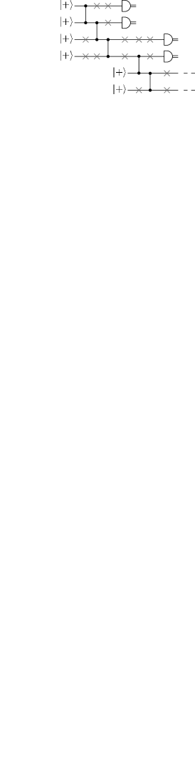
Figure 40: The literal circuit for a two-at-a-time implementation of a single-qubit cluster-state computation, with the noisy quantum memory steps explicitly indicated by crosses. For simplicity we have combined the single-qubit rotations and computational basis measurements into a single-qubit measurement in some other basis, not explicitly specified.

Commuting the operations in Figure 40 forward in time, we see that that the output of Figure 40 is equivalent to the output of the circuit in Figure 41. Note that doing this commutation requires the use of Proposition 4, since noisy operations on different qubits that are on the same level of the cluster may potentially involve the same environment, and so may not commute. Fortunately, Proposition 4 allows this commutation to be performed without increasing the strength of the underlying noise.

Inspection of Figure 41 reveals that this circuit may be regarded as the literal circuit for a one-buffered implementation of a cluster-state computation, and thus is equivalent to a noisy quantum circuit, using the results of Section IV. A similar argument can be used to map noise in a multi-qubit two-at-a-time implementation of a cluster-state computation to equivalent noise in a quantum circuit. We omit the details of the argument, which is a straightforward extension of the single-qubit case.

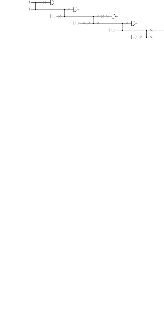
Figure 41: The output of this circuit is equivalent to the output of the literal circuit for the two-at-a-time implementation in Figure 40.

V.4 Postselected gates

In order to map noise in optical cluster-state computation into the quantum circuit model, we need a simple lemma about postselected quantum gates. In this subsection we provide a formal definition of what we call a unitary postselected gate, and prove the required lemma. The unitary postselected gates discussed here differ in an important respect from the postselected gates in the discussion of optical quantum computing in Section III. In the optical gates, success of the quantum gate is conditional on some measurement outcome occurring. In the present scenario the postselected gate is all-unitary, i.e., no measurement is involved. The connection between the two types of postselection is made by replacing the measurement by an equivalent unitary process; we will see an explicit example of how this works in the next subsection.

Let $U$ be a unitary gate acting on two registers, labeled $A$ and $B$. $B$ is initially in some fixed state $|\beta\rangle$, while $A$ may be in an arbitrary state $|\psi\rangle$. Let $V$ be a unitary gate acting on register $A$ alone. $U$ is said to be a unitary postselected gate that implements $V$ with probability $p$ if for all $|\psi\rangle$,

$$U|\psi\rangle|\beta\rangle=\sqrt{p}V|\psi\rangle|\beta^{\prime}\rangle+\sqrt{1-p}|\psi^{\prime}\rangle|\beta^{\prime\prime}\rangle,$$ (30)

where $|\beta^{\prime}\rangle$ is some fixed state, and $|\beta^{\prime\prime}\rangle$ is orthonormal to $|\beta^{\prime}\rangle$.

Lemma 1

Let $U$ be a unitary postselected gate implementing $V$ with probability $p$, on registers $A$ and $B$, and when $|\beta\rangle$ is input to the register $B$. Let $S$ be a subspace of the state space for register $A$, and let $T$ be the subspace of the total state space for $AB$ that contains states of the form $|\psi\rangle|\beta\rangle$, where $|\psi\rangle\in S$. Then there exists a unitary $W$ acting on register $B$ such that

$$\|U|_{T}-(V\otimes W)|_{T}\|=\sqrt{2(1-\sqrt{p})}.$$ (31)

Proof: By definition, for all states $|\psi\rangle$ in register $A$ we have

$$U|\psi\rangle|\beta\rangle=\sqrt{p}V|\psi\rangle|\beta^{\prime}\rangle+\sqrt{1-p}|\psi^{\prime}\rangle|\beta^{\prime\prime}\rangle.$$ (32)

Let $W$ be a unitary operator taking $|\beta\rangle$ to $|\beta^{\prime}\rangle$. Then

$$(U-V\otimes W)|\psi\rangle|\beta\rangle = (\sqrt{p}-1)V|\psi\rangle|\beta^{\prime}\rangle$$ (33)

$$+\sqrt{1-p}|\psi^{\prime}\rangle|\beta^{\prime\prime}\rangle.$$

Evaluating the norm, and restricting to normalized states $|\psi\rangle|\beta\rangle$ which are in $T$, we obtain the result.

QED

V.5 How noise in optical cluster-state computation maps to noise in the quantum circuit model

In this subsection we explain how noise in the dangling node implementation of optical cluster-state computation is mapped to equivalent noise in the two-at-a-time implementation described in Subsection V.3. The results in Subsection V.3 may then be used to map that noise to equivalent noise in the original quantum circuit, which enables us to complete the threshold proof. Our main focus here is on noise in single-qubit cluster-state computations, since the multi-qubit case follows similar lines, and requires no new ideas.

Consider a dangling node implementation of a single-qubit cluster-state computation. The literal circuit for such a computation is depicted in Figure 42. The first step of the circuit sets up the initial microcluster. The remaining steps of the circuit alternate between applications of the operation add, which effectively adds two extra layers of qubits to the cluster, and the operation measure, which implements the desired single-qubit measurements and feedforward of measurement results. (Note that we have omitted ancillas, classical processing of data, and feedforward from the visual depiction, for simplicity.)

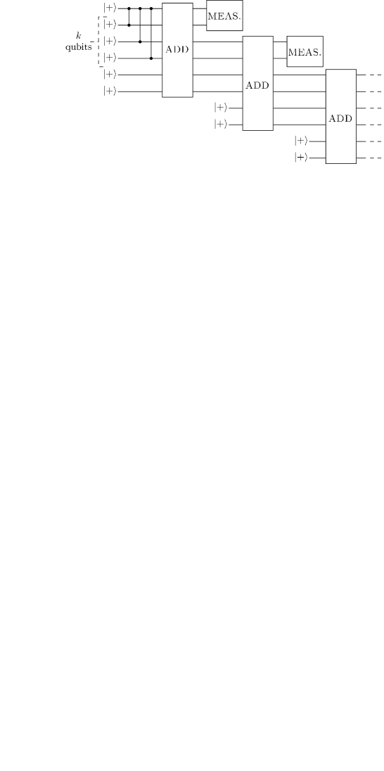
Figure 42: The literal circuit for a dangling node implementation of a single-qubit cluster-state computation. We have chosen to use an implementation with $k=3$ dangling nodes; the circuit for other values of $k$ follows similar lines.

The operation add may be broken down into the following operations:

• Preparation of microcluster states which we attempt to adjoin to the existing cluster.

• All quantum gates applied in the process of attempting to adjoin the additional microclusters, including non-deterministic cphase gates.

• Ancillas used in the non-deterministic cphase gates.

• All the classical control and feedforward.

• The computational basis measurements and local $Z$ operations needed to remove undesired qubits from the cluster.

In addition to these physical operations, to simplify the analysis it is convenient to append some fictitious perfect controlled-swap operations to ensure that the effective output qubits always appear on the same output lines. That is, these controlled-swap operations effectively change the labels on the qubits to ensure that the same qubits always act as the output, but otherwise don’t affect the output state. The operations are chosen so that the approximate circuit identity illustrated in Figure 43 holds. This identity illustrates the fact that the result of attempting to add two extra layers of qubits to the cluster of Figure 32 results, with high probability, in the cluster of Figure 33. The identity fails to be exact because (a) the attempt to add extra layers sometimes fails, resulting (even in the ideal case of perfect operations) in the cluster of Figure 34, and (b) the physical operations used are inevitably somewhat noisy.

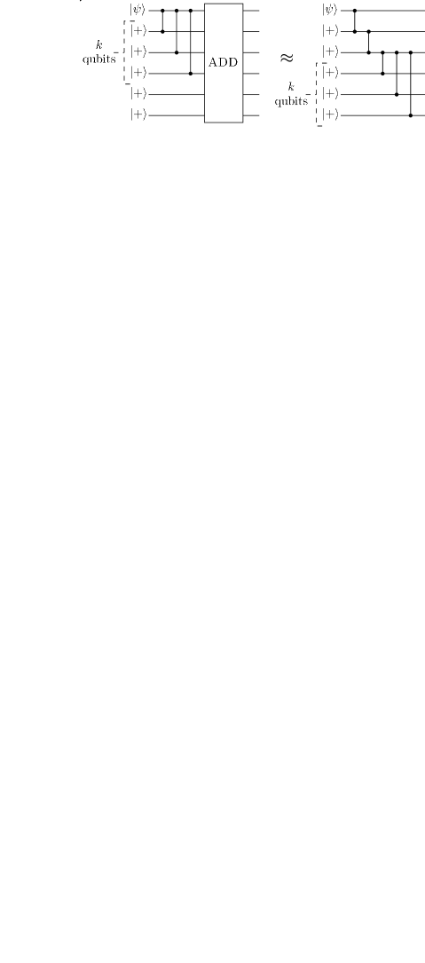
Figure 43: The operation add satisfies the approximate circuit identity illustrated here. This identity becomes more exact as $k$ is increased, and the level of noise in the physical operations used to do the operation is decreased.

The next step of the proof is to replace the measurements, classical control and feedforward performed in the add operation by equivalent ancilla preparations and unitary quantum operations, in a similar fashion to our threshold proof for deterministic cphase gates in Section IV. The result is an operation qadd, involving only quantum systems, perfect ancilla preparation, and noisy unitary operations. Note that, once again, we model noisy ancilla preparation by perfect ancilla preparation, followed by a noisy quantum memory step. The output of the noisy dangling node cluster-state computation is thus the same as the output of the imperfect circuit illustrated in Figure 44.

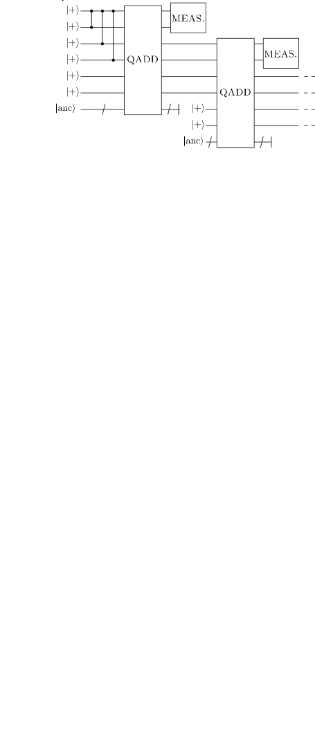
Figure 44: The output of this imperfect circuit is the same as the output of the noisy cluster-state computation. The state $|{\rm anc}\rangle$ is an ancilla prepared (noisily) offline; it contains microclusters, the ancillas used in the KLM cphase, and qubits used to simulate the classical control and feedforward in the dangling node implementation. Note that the ancilla line is marked by a slash to indicate that it involves many systems, not just a single qubit.

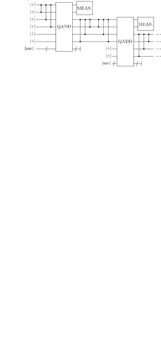
Figure 45: We may insert some fictitious perfect gates between the operations in Figure 44, without changing the output.

As in the deterministic case, we may insert fictitious perfect extra gates between qadd operations without changing the overall output, as illustrated in Fig 45. The entire noisy cluster-state computation is thus equivalent to the repeating circuit illustrated in Figure 46, where the gate $G$ is as defined in Figure 47.

In our analysis it is convenient to distinguish between the perfect gate $G$, and the imperfect gate $G_{n}$, which also includes the effects of noise due to interactions with the environment, $E$. Note that due to the chaining property, $\Delta_{Q:AE}(G,G_{n})\leq N\eta$, where the systems $Q$ and $A$ are as defined in Figure 47, $N$ is the total number of noisy operations involved in the operation $G_{n}$, and $\eta$ is the maximal noise strength of any of those operations. Simple counting shows that $N\leq c_{1}k^{2}$ for some positive constant $c_{1}$ in the range $10^{0}$-$10^{2}$, and so $\Delta_{Q:AE}(G,G_{n})\leq c_{1}k^{2}\eta$.

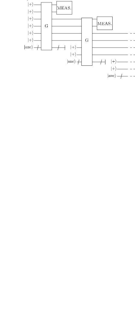
Figure 46: The output of this imperfect circuit is the same as the output of the noisy dangling node cluster-state computation.

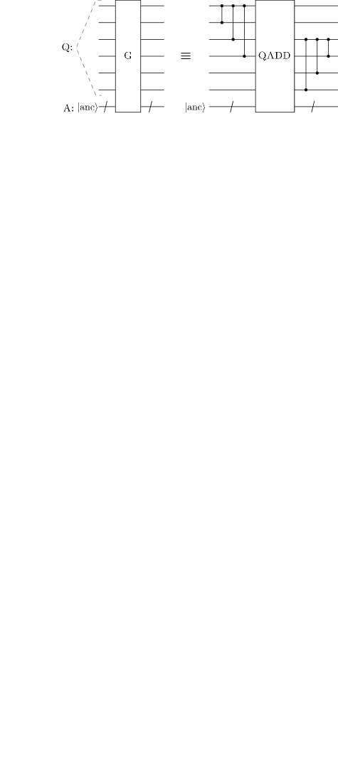
Figure 47: The definition of the gate $G$ used in Figure 46. This figure also defines subsystem labels $Q$ and $A$.

With these definitions we see that $G$ is a unitary postselected gate acting on the registers $Q$ and $A$, implementing the gate $V$ defined in Figure 48 on register $Q$, with probability $p_{s}=1-p_{f}^{k-1}$. Let $S$ be the subspace of states for $Q$ of the form $|\psi\rangle|+\rangle\ldots|+\rangle$, where $|\psi\rangle$ is an arbitrary single-qubit state. Let $T$ be the subspace of states for the system $QA$ which are of the form $|\phi\rangle|{\rm anc}\rangle$, where $|\phi\rangle$ is any state in $S$, and $|{\rm anc}\rangle$ is the initial state of the ancilla $A$. It is also useful to define $T^{\prime}$ to be the subspace of the combined system $QAE$ containing states of the form $|\phi\rangle_{SE}\otimes|{\rm anc}\rangle$, where $|\phi\rangle_{SE}$ is an arbitrary state in $S\otimes E$. Applying Lemma 1, we conclude that there exists a unitary $W$ acting on $A$ such that

$$\|G|_{T}-(V\otimes W)|_{T}\|=\sqrt{2(1-\sqrt{p_{s}})}.$$ (34)

Recalling that $\Delta_{Q:AE}(G,G_{n})\leq c_{1}k^{2}\eta$, we see that there exists unitary $G_{E}$ acting on $E$ such that

$$\|G_{n}-G\otimes G_{E}\|\leq c_{1}k^{2}\eta.$$ (35)

Restricting to the subspace $T^{\prime}$ we have

$$\|G_{n}|_{T^{\prime}}-(G\otimes G_{E})|_{T^{\prime}}\|\leq c_{1}k^{2}\eta.$$ (36)

From Eq. (34) we deduce that

$$\|(G\otimes G_{E})|_{T^{\prime}}-(V\otimes W\otimes G_{E})|_{T^{\prime}}\|=\sqrt{2(1-\sqrt{p_{s}})}.$$

(37)

Using the triangle inequality and Eqs. (36) and (37) we obtain

$$\|G_{n}|_{T^{\prime}}-(V\otimes W\otimes G_{E})|_{T^{\prime}}\|\leq c_{1}k^{2}\eta+\sqrt{2(1-\sqrt{p_{s}})}.$$

Applying the second unitary extension theorem, Theorem 2, we see that there exists unitary $\tilde{G}_{n}$ whose action on $T^{\prime}$ is identical to the action of $G_{n}$, and such that

$$\|\tilde{G}_{n}-(V\otimes W\otimes G_{E})\| \leq 2c_{1}k^{2}\eta+2\sqrt{2(1-\sqrt{p_{s}})}.$$

Figure 48: The definition of the gate $V$.

Summarizing, the output of the noisy cluster-state computation is the same as the output of the noisy circuit in Figure 49. The blocks of two imperfect cphase gates shown in this circuit represent the operation $\tilde{G}_{n}$, which we have seen satisfies

$$\Delta_{Q:AE}(V,\tilde{G}_{n})\leq 2c_{1}k^{2}\eta+2\sqrt{2(1-\sqrt{p_{s}})},$$ (40)

where $p_{s}=1-p_{f}^{k-1}$ is the probability of successfully adjoining a microcluster, and $p_{f}$ is the probability of a non-deterministic cphase failing. Examining Figure 49, we see that a dangling node implementation using non-deterministic gates is equivalent to a noisy two-at-a-time deterministic implementation, where the additional layers of the cluster are added with noise of total strength at most $2c_{1}k^{2}\eta+2\sqrt{2(1-\sqrt{p_{s}})}$. Combining this with the results about the two-at-a-time implementation in Subsection V.3, we see that a noisy dangling node implementation of a single-qubit cluster-state computation is equivalent to a noisy single-qubit quantum circuit computation. Noise of strength $\eta$ in the dangling node implementation is mapped to equivalent noise of strength $c_{1}k^{2}\eta+c_{2}\eta+2\sqrt{2(1-\sqrt{p_{s}})}$ in the quantum circuit model of computation, where the extra contribution $c_{2}\eta$ is due to noise in the single-qubit measurements, and $c_{2}$ is a positive constant of order $10^{0}$.

Figure 49: The output of this noisy circuit is the same as the output of the noisy cluster-state computation.

Similar reasoning can be used to map noise of strength $\eta$ in a dangling node implementation of a multi-qubit cluster-state computation back to the original quantum circuit with noise of strength at most $c_{1}k^{2}\eta+c_{2}\eta+2\sqrt{2(1-\sqrt{p_{s}})}$, where the constants $c_{1}$ and $c_{2}$ may now be different, but are still of the same order, and $p_{s}=1-2p_{f}^{k-1}+p_{f}^{2k-2}$. The only difference in the proof is that in addition to the $G$ operations, multi-qubit computations also involve analogous operations based on the process of adjoining the more complex microcluster of Figure 36. However, the analysis for such operations goes through in exactly the same way as in the single-qubit case.

Summing up, we have shown that noise of strength up to $\eta$ in a dangling node implementation of a cluster-state computation is equivalent to noise of strength at most $c_{1}k^{2}\eta+c_{2}\eta+2\sqrt{2(1-\sqrt{p_{s}})}$ in the original quantum circuit, where $c_{1}$ is a positive constant of order $10^{0}$-$10^{2}$, $c_{2}$ is a positive constant of order $10^{0}$, and $p_{s}=1-2p_{f}^{k-1}+p_{f}^{2k-2}$. Thus, provided $k$ and $\eta$ satisfy

$$c_{1}k^{2}\eta+c_{2}\eta+2\sqrt{2(1-\sqrt{p_{s}})}\leq\eta_{\rm th}$$ (41)

it is possible to compute fault-tolerantly in the optical cluster-state proposal for computation. This may be rephrased as the condition:

$$\eta\leq\eta_{k,{\rm th}}^{\rm ocs}\equiv\frac{\eta_{\rm th}-2\sqrt{2(1-\sqrt{p_{s}})}}{c_{1}k^{2}+c_{2}}.$$ (42)

We can always ensure that $\eta_{k,{\rm th}}^{\rm ocs}>0$ by choosing $k$ sufficiently large. Provided this condition is satisfied, $\eta_{k,{\rm th}}^{\rm ocs}$ is thus a threshold for optical cluster-state computation.

VI Conclusion

In this paper we have proved two fault-tolerant threshold theorems for the cluster-state model of quantum computation. Our first threshold theorem applies to implementations in which deterministic (but noisy) entangling gates are available. Our second threshold theorem is specifically adapted to the case of optical quantum computation, where entangling gates are performed non-deterministically. In both cases our threshold theorems hold for quite pessimistic noise models, allowing non-Markovian noise applied by an intelligent adversary who can exploit constructive interference to enhance the effects of the noise, and even cause errors in the classical computation and feedforward of measurement results. A drawback of our noise models is that they do not yet allow the possibility of leakage errors, like photon loss in optics. We expect to remove this drawback in future work, by combining the ideas in Terhal and Burkard (2004) with well-established methods for dealing with photon loss, e.g. Knill et al. (2000).

Our focus has been on proving that a finite threshold exists for cluster-state computation, rather than on obtaining a precise numerical evaluation of the threshold. This is consistent with our general philosophy of understanding the threshold through a two-part process: first, rigorously proving the existence of a finite threshold for some large class of noise models; and second, through a combination of numerical and analytic work obtaining a realistic estimate of the threshold for some specific and physically-motivated noise model. In this paper we have obtained a rigorous proof that a finite threshold exists. Detailed numerical simulation and optimization of the threshold value for realistic noise models is underway, and will be reported elsewhere Dawson et al. .

Our investigations in this paper have been geared toward variants of the one-way quantum computing model introduced by Raussendorf and Briegel Raussendorf and Briegel (2001). However, the techniques we have proposed seem quite generally applicable to the task of making measurement-based schemes for quantum computation fault-tolerant. It seems likely that schemes such as those proposed in Nielsen (2003a); Yoran and Reznik (2003); Jorrand and Perdrix (2004); Childs et al. (2004) (see also references therein) can be made fault-tolerant using similar ideas. Particularly appealing from a theoretical point of view is the possibility of fault-tolerant computation using measurement alone, with no unitary gates whatsoever (excepting quantum memory). This might be done using, for example, a scheme such as Nielsen (2003a), or one of the simpler variants that has since been proposed Fenner and Zhang (2001); Leung (2001, 2003); Perdrix (2004).

The most important conclusion from our results is that noise need not be an obstacle to scalable quantum computation using cluster states. In particular, our results provide encouraging evidence that practical proposals for cluster-state quantum computation using neutral atoms Raussendorf and Briegel (2001) and optics Nielsen (2004) are, in principle, fully scalable approaches to quantum computation.

Appendix A The unitary extension theorems

In this appendix we restate and prove the first and second unitary extension theorems, from Section II.1.

Theorem 5

(First unitary extension theorem) Let $U,\tilde{U}$ and $V$ be unitaries acting on a Hilbert space $T$. Suppose $S$ is a subspace of $T$ such that $U$ and $\tilde{U}$ have the same action on $S$, i.e., $U|_{S}=\tilde{U}|_{S}$. (Note that we do not assume that $U$ and $\tilde{U}$ leave the subspace $S$ invariant, so $U|_{S}$ and $\tilde{U}|_{S}$ should be considered as maps from $S$ into $T$.) Then there exists a unitary extension $\tilde{V}$ of $V|_{S}$ to the entire space $T$ such that

$$\|\tilde{V}-\tilde{U}\|\leq\|V-U\|.$$ (43)

It is worth noting that the proof below holds not just for the matrix norm, but for any norm such that $\|AB\|\leq\|A\|\,\|B\|$, and $\|W\|\leq 1$ for all unitaries $W$.

Proof: Let $P$ be the projector onto the subspace $S$, and let $Q=I-P$ be the projector onto the orthocomplement of $S$ in $T$. Define

$$\tilde{V}\equiv VP+VU^{\dagger}\tilde{U}Q.$$ (44)

We will show that $\tilde{V}$ has the required properties. It is clear that $\tilde{V}$ is an extension of $V|_{S}$. To prove unitarity of $\tilde{V}$ we first observe that

$$U^{\dagger}\tilde{U}Q=QU^{\dagger}\tilde{U}.$$ (45)

To prove this equation, observe that it is equivalent to $U^{\dagger}\tilde{U}P=PU^{\dagger}\tilde{U}$, since $Q=I-P$. But $U^{\dagger}\tilde{U}P=PU^{\dagger}\tilde{U}$ follows easily from the fact that $U|_{S}=\tilde{U}|_{S}$. The unitarity of $\tilde{V}$ follows from Eqs. (44), (45), and some algebra:

$$\tilde{V}\tilde{V}^{\dagger} = VPV^{\dagger}+V(U^{\dagger}\tilde{U})Q(U^{\dagger}\tilde{U})^{\dagger}V^{\dagger}$$ (46)

$$= VPV^{\dagger}+VQV^{\dagger}$$ (47)

$$= VV^{\dagger}$$ (48)

$$= I.$$ (49)

To bound $\|\tilde{V}-\tilde{U}\|$ observe that

$$\tilde{V}-\tilde{U} = VP+VU^{\dagger}\tilde{U}Q-\tilde{U}P-\tilde{U}Q.$$ (50)

Observing that $\tilde{U}P=UP$ and inserting $UU^{\dagger}=I$ we get

$$\tilde{V}-\tilde{U} = VP+VU^{\dagger}\tilde{U}Q-UP-UU^{\dagger}\tilde{U}Q$$ (51)

$$= (V-U)(P+U^{\dagger}\tilde{U}Q).$$ (52)

Recall that $\|AB\|\leq\|A\|\,\|B\|$, and observe that $P+U^{\dagger}\tilde{U}Q$ is unitary. It follows that $\|P+U^{\dagger}\tilde{U}Q\|=1$, and thus $\|\tilde{V}-\tilde{U}\|\leq\|V-U\|$, as required.

QED

Theorem 6

(Second unitary extension theorem) Let $U$ and $V$ be unitary operations acting on a (finite-dimensional) inner product space $T$. Suppose $S$ is a subspace of $T$. Then there exists a unitary operation $\tilde{V}$ such that $\tilde{V}|_{S}=V|_{S}$ and

$$\|U-\tilde{V}\|\leq 2\|U|_{S}-V|_{S}\|.$$ (53)

The proof of the second unitary extension theorem is somewhat more complex than the proof of the first. We begin the proof by introducing some notation related to the singular value decomposition of a matrix, and then we state and prove some simple lemmas about singular values and matrix norms.

Recall that the singular value decomposition states that an arbitrary $m\times n$ matrix $M$ can be written $M=L_{M}\Sigma_{M}R_{M}$, where $L_{M}$ is an $m\times m$ unitary matrix, $R_{M}$ is an $n\times n$ unitary matrix, and $\Sigma_{M}$ is an $m\times n$ matrix, all of whose entries are zero, except the diagonal entries $(\Sigma_{M})_{jj}=\sigma_{j}(M)$, known as the singular values, which are non-negative and arranged in decreasing order, $\sigma_{1}(M)\geq\sigma_{2}(M)\geq\ldots$. It is easy to see that the singular values are determined by the equation $\sigma_{j}(M)^{2}=\lambda_{j}(M^{\dagger}M)=\lambda_{j}(MM^{\dagger})$, the $j$th largest eigenvalues of the matrices $M^{\dagger}M$ and $MM^{\dagger}$. It is also useful to note that $\|M\|=\sigma_{1}(M)$. When $M$ is an $m\times m$ matrix (i.e., a square matrix), we will use the notation $\sigma_{\min}(M)\equiv\sigma_{m}(M)$ to denote the smallest singular value of $M$.

Proposition 7

Suppose $U$ is a unitary matrix that can be written

$$U=\left[\begin{array}[]{cc}A&C\\ B&D\end{array}\right],$$ (56)

where $A$ is an $m\times m$ matrix, $B$ is $n\times m$, $C$ is $m\times n$, and $D$ is $n\times n$. Then $\sigma_{\min}(A)=\sigma_{\min}(D)$.

Proof: Inspection of the equations $U^{\dagger}U=UU^{\dagger}=I$ implies that $A^{\dagger}A+B^{\dagger}B=I_{m}$ and $BB^{\dagger}+DD^{\dagger}=I_{n}$, where we use $I_{k}$ to denote the $k\times k$ identity matrix. Using these equations we have:

$$\sigma_{\min}(A)^{2} = \lambda_{m}(A^{\dagger}A)$$ (57)

$$= 1-\lambda_{1}(B^{\dagger}B)$$ (58)

$$= 1-\lambda_{1}(BB^{\dagger})$$ (59)

$$= \lambda_{n}(DD^{\dagger})$$ (60)

$$= \sigma_{\min}(D)^{2},$$ (61)

from which the result follows. An alternate proof of this proposition follows immediately from the well-known CS decomposition of linear algebra (see, for example, Theorem VII.1.6 on page 196 of Bhatia (1997)).

QED

To state the next proposition we need to introduce some additional notation. We define the partial order $X\leq Y$ for matrices $X$ and $Y$ if $Y-X$ is a positive matrix. We define $|X|\equiv\sqrt{X^{\dagger}X}$.

Proposition 8

Suppose $M$ is a matrix such that $|M|\leq I$. Then $\|I-M\|\geq 1-\sigma_{\min}(M)$.

Proof: Choose a normalized vector $|\psi\rangle$ so that $\Sigma_{M}|\psi\rangle=\sigma_{\min}(M)|\psi\rangle$. By the singular value decomposition $\|I-M\|=\|I-L_{M}\Sigma_{M}R_{M}\|=\|W-\Sigma_{M}\|$, where $W\equiv L_{M}^{\dagger}R_{M}^{\dagger}$. Thus

$$\|I-M\| \geq \|(W-\Sigma_{M})|\psi\rangle\|$$ (62)

$$\geq \|W|\psi\rangle\|-\|\Sigma_{M}|\psi\rangle\|$$ (63)

$$= 1-\sigma_{\min}(M),$$ (64)

where we have used the triangle inequality.

QED

Proposition 9

Let

$$M=\left[\begin{array}[]{cc}A&B\\ B^{\dagger}&C\end{array}\right]$$ (67)

be a positive (and thus Hermitian) square matrix. We assume $A$ is $m\times m$, $B$ is $m\times n$, and $C$ is $n\times n$. Then

$$\|M\|\leq\|A\|+\|C\|.$$ (68)

Proof: This proposition can be viewed as a special case of Aronszajn’s inequality, Theorem III.2.9 on page 64 of Bhatia (1997). Alternately, since $M$ is positive we can find a block matrix $D=[D_{1}D_{2}]$ such that $M=D^{\dagger}D$, and thus $A=D_{1}^{\dagger}D_{1}$ and $C=D_{2}^{\dagger}D_{2}$. We have

$$\|M\| = \lambda_{1}(D^{\dagger}D)$$ (69)

$$= \lambda_{1}(DD^{\dagger})$$ (70)

$$= \lambda_{1}(D_{1}D_{1}^{\dagger}+D_{2}D_{2}^{\dagger})$$ (71)

$$\leq \lambda_{1}(D_{1}D_{1}^{\dagger})+\lambda_{1}(D_{2}D_{2}^{\dagger})$$ (72)

$$= \|A\|+\|B\|,$$ (73)

where the second-last line follows from the well-known eigenvalue inequality $\lambda_{1}(A+B)\leq\lambda_{1}(A)+\lambda_{1}(B)$, true for all Hermitian matrices $A$ and $B$.

QED

Proof of the second unitary extension theorem: We prove the theorem in two parts. In the first part we prove the result for the case $U=I$. In the second part we show that the general result follows from the case when $U=I$.

For the first part, we write $V$ in block-diagonal form as

$$V=\left[\begin{array}[]{cc}A&C\\ B&D\end{array}\right],$$ (76)

where the first block represents a basis for $S$, and the second block represents a basis for the orthocomplement $S_{\perp}$. Let the singular value decomposition of $D$ be $D=L_{D}\Sigma_{D}R_{D}$. Rotating by $L_{D}^{\dagger}$ to change the basis of $S_{\perp}$ we see that $V$ can be written in the new basis as

$$V=\left[\begin{array}[]{cc}A^{\prime}&C^{\prime}\\ B^{\prime}&\Sigma_{D}R_{D}L_{D}\end{array}\right],$$ (79)

where $A^{\prime},B^{\prime},C^{\prime}$ represent the action of $V$ with respect to the new basis. We define the extension $\tilde{V}$ by

$$\tilde{V} \equiv V\left[\begin{array}[]{cc}I&0\\ 0&L_{D}^{\dagger}R_{D}^{\dagger}\end{array}\right]$$ (82)

$$= \left[\begin{array}[]{cc}A^{\prime}&C^{\prime\prime}\\ B^{\prime}&\Sigma_{D}\end{array}\right],$$ (85)

where $C^{\prime\prime}=C^{\prime}L_{D}^{\dagger}R_{D}^{\dagger}$. It is clear that $\tilde{V}$ is unitary and $\tilde{V}|_{S}=V_{S}$. All that remains to complete the first part of the proof is to bound $\|\tilde{V}-I\|$. We have

$$\|\tilde{V}-I\|^{2} = \|(\tilde{V}-I)(\tilde{V}^{\dagger}-I)\|$$ (86)

$$= \|2I-\tilde{V}-\tilde{V}^{\dagger}\|$$ (87)

$$= \left\|\left[\begin{array}[]{cc}2I-A^{\prime}-A^{\prime\dagger}&-C^{\prime\prime}-B^{\prime\dagger}\\ -B^{\prime}-C^{\prime\prime\dagger}&2I-2\Sigma_{D}\end{array}\right]\right\|.$$ (90)

Applying Proposition 9 we obtain

$$\|\tilde{V}-I\|^{2}\leq\|2I-A^{\prime}-A^{\prime\dagger}\|+\|2I-2\Sigma_{D}\|.$$ (92)

But $\|2I-A^{\prime}-A^{\prime\dagger}\|\leq\|I-A^{\prime}\|+\|I-A^{\prime\dagger}\|=2\|I-A^{\prime}\|\leq 2\|I|_{S}-V|_{S}\|$. We also have $\|2I-2\Sigma_{D}\|=2-2\sigma_{\min}(D)=2-2\sigma_{\min}(A^{\prime})\leq 2\|I-A^{\prime}\|\leq 2\|I|_{S}-V|_{S}\|$. The first part of the proof follows.

For the second part of the proof we set $U^{\prime}\equiv I,V^{\prime}\equiv U^{\dagger}V$. Then by the first part of the proof there exists unitary $\tilde{V}^{\prime}$ such that $\tilde{V}^{\prime}|_{S}=U^{\dagger}V|_{S}$, and $\|\tilde{V}^{\prime}-I\|\leq 2\|U^{\dagger}V|_{S}-I_{S}\|$. Set $\tilde{V}\equiv U\tilde{V}^{\prime}$. Then $\tilde{V}$ is a unitary matrix such that $\tilde{V}|_{S}=V|_{S}$ and

$$\|\tilde{V}-U\| = \|\tilde{V}^{\prime}-I\|$$ (93)

$$\leq 2\|U^{\dagger}V|_{S}-I|_{S}\|$$ (94)

$$= 2\|V|_{S}-U|_{S}\|.$$ (95)

QED

An alternate proof of the second unitary extension theorem may be given, following similar lines, but based on the well-known CS decomposition from linear algebra. We have taken the approach presented here as it is only slightly more complex than the alternate proof, and relies on less background material.

Appendix B Proof of Proposition 5

In this appendix we prove Proposition 5, which asserts the truth of the circuit identity in Figure 23. This proposition establishes the correspondence between blocks $QB_{\alpha}$ and gates $HZ_{\alpha}$ in the quantum circuit.

To prove Proposition 5 we make use of four simple circuit identities which we assert here without proof. Each may be readily verified by direct computation. The first identity is a simplification of a common element in literal circuits for cluster-state computation.

Identity 1

The following circuit simplification holds where the second qubit is in the state $|+\rangle$.

The remaining three identities concern the commutativity properties of cnot (controlled-not) and cphase gates when the control of one operator is the target of the operator immediately following or preceding it.

Identity 2

The following circuit identity holds:

Identity 3

The following circuit identity holds:

Identity 4

The following circuit identity holds:

With these identities we can now prove Proposition 5. The proof is a short sequence of circuit identities which are shown in Figure 50.

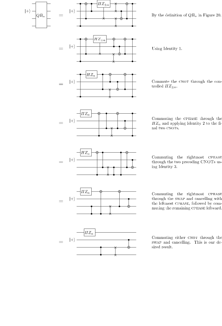
Figure 50: The sequence of circuit identities used to prove Proposition 5

References

- Raussendorf and Briegel (2001) R. Raussendorf and H. J. Briegel, Phys. Rev. Lett. 86, 5188 (2001).
- Nielsen (2003a) M. A. Nielsen, Phys. Lett. A 308, 96 (2003a), arXiv:quant-ph/0108020.
- Nielsen and Chuang (2000) M. A. Nielsen and I. L. Chuang, Quantum computation and quantum information (Cambridge University Press, Cambridge, 2000).
- Bennett et al. (1993) C. H. Bennett, G. Brassard, C. Crépeau, R. Jozsa, A. Peres, and W. K. Wootters, Phys. Rev. Lett. 70, 1895 (1993).
- Nielsen and Chuang (1997) M. A. Nielsen and I. L. Chuang, Phys. Rev. Lett. 79, 321 (1997).
- Gottesman and Chuang (1999) D. Gottesman and I. L. Chuang, Nature 402, 390 (1999), arXiv:quant-ph/9908010.
- Aliferis and Leung (2004) P. Aliferis and D. W. Leung, arXiv:quant-ph/0404082 (2004).
- Jorrand and Perdrix (2004) P. Jorrand and S. Perdrix, arXiv:quant-ph/0404125 (2004).
- Childs et al. (2004) A. M. Childs, D. W. Leung, and M. A. Nielsen, arXiv:quant-ph/0404132 (2004).
- Nielsen (2004) M. A. Nielsen (2004), arXiv:quant-ph/0402005, accepted to Phys. Rev. Lett.
- Raussendorf (2003) R. Raussendorf, Ph.D. thesis, Ludwig-Maximillians Universität München (2003), http://edoc.ub.uni-muenchen.de/archive/00001367.
- (12) R. Raussendorf and H. Briegel, private communcation (2004).
- Yamamoto et al. (1988) Y. Yamamoto, M. Kitagawa, and K. Igeta, in Proc. 3rd Asia-Pacific Phys. Conf. (World Scientific, Singapore, 1988).
- Milburn (1989) G. J. Milburn, Phys. Rev. Lett. 62, 2124 (1989).
- Knill et al. (2001) E. Knill, R. Laflamme, and G. J. Milburn, Nature 409, 46 (2001).
- Pittman et al. (2003) T. B. Pittman, M. J. Fitch, B. C. Jacobs, and J. D. Franson, Phys. Rev. A 68, 032316 (2003).
- O’Brien et al. (2003) J. L. O’Brien, G. J. Pryde, A. G. White, T. C. Ralph, and D. Branning, Nature 426, 264 (2003).
- Sanaka et al. (2003) K. Sanaka, T. Jennewein, J.-W. Pan, K. Resch, and A. Zeilinger, Phys. Rev. Lett. 92, 017902 (2003), arXiv:quant-ph/0308134.
- Gasparoni et al. (2004) S. Gasparoni, J.-W. Pan, P. Walther, T. Tudolph, and A. Zeilinger, arXiv:quant-ph/0404107 (2004).
- Zhao et al. (2004) Z. Zhao, A.-N. Zhang, Y.-A. Chen, H. Zhang, J.-F. Du, T. Yang, and J.-W. Pan, arXiv:quant-ph/0404129 (2004).
- Yoran and Reznik (2003) N. Yoran and B. Reznik, Phys. Rev. Lett. 91, 037903 (2003), arXiv:quant-ph/0303008.
- Knill (2004a) E. Knill, arXiv:quant-ph/0402171 (2004a).
- Knill (2004b) E. Knill, arXiv:quant-ph/0404104 (2004b).
- Steane (2002) A. M. Steane, arXiv:quant-ph/0207119 (2002).
- Steane and Ibinson (2003) A. M. Steane and B. Ibinson, arXiv:quant-ph/0311014 (2003).
- Dür and Briegel (2003) W. Dür and H.-J. Briegel, Phys. Rev. Lett. 90, 067901 (2003), arXiv:quant-ph/0210069.
- (27) C. Dawson, H. L. Haselgrove, and M. A. Nielsen, in preparation.
- Terhal and Burkard (2004) B. M. Terhal and G. Burkard, arXiv:quant-ph/0402104 (2004).
- Aharonov and Ben-Or (1997) D. Aharonov and M. Ben-Or, in Proceedings of the Twenty-Ninth Annual ACM Symposium on the Theory of Computing (1997), pp. 176–188.
- Aharonov and Ben-Or (1999) D. Aharonov and M. Ben-Or, arXiv:quant-ph/9906129 (1999).
- Aharonov et al. (1996) D. Aharonov, M. Ben-Or, R. Impagliazzo, and N. Nisan, arXiv:quant-ph/9611028 (1996).
- Nielsen (2003b) M. A. Nielsen (2003b), available at http://www.qinfo.org/qc-by-measurement/.
- Raussendorf and J.Briegel (2002) R. Raussendorf and H. J.Briegel, J. Mod. Opt. 49, 1299 (2002), arXiv:quant-ph/0108067.
- Raussendorf et al. (2003) R. Raussendorf, D. E. Browne, and H. J. Briegel, Phys. Rev. A 68, 022312 (2003), arXiv:quant-ph/0108118.
- Fenner and Zhang (2001) S. A. Fenner and Y. Zhang, arXiv:quant-ph/0111077 (2001).
- Leung (2001) D. W. Leung, arXiv:quant-ph/0111122 (2001).
- Leung (2003) D. W. Leung, arXiv:quant-ph/0310189 (2003).
- Jorrand and Perdrix (2003) P. Jorrand and S. Perdrix, arXiv:quant-ph/0311142 (2003).
- Perdrix and Jorrand (2004a) S. Perdrix and P. Jorrand, arXiv:quant-ph/0402156 (2004a).
- Perdrix (2004) S. Perdrix, arXiv:quant-ph/0402204 (2004).
- Perdrix and Jorrand (2004b) S. Perdrix and P. Jorrand, arXiv:quant-ph/0404146 (2004b).
- Knill et al. (2000) E. Knill, R. Laflamme, and G. J. Milburn, arXiv:quant-ph/0006120 (2000).
- Bhatia (1997) R. Bhatia, Matrix analysis (Springer-Verlag, New York, 1997).