Spatial weak-light solitons in an electro-magnetically induced nonlinear waveguide

Abstract

We show that a weak probe light beam can form spatial solitons in an electro-magnetically induced transparency (EIT) medium composed of four-level atoms and a coupling light field. We find that the coupling light beam can induce a highly controllable nonlinear waveguide and exert very strong effects on the dynamical behaviors of the solitons. Hence, in the EIT medium, it is not only possible to produce spatial solitons at very low light intensities but also simultaneously control these solitons by using the coupling-light-induced nonlinear waveguide.

Finding new physical systems for producing optical solitons at very low light intensities with good controllabilities is very important for investigating the nonlinear dynamics of quantum solitons and inventing new optical devices for quantum or conventional optical communications and computations YamamotoNature ; KavisharReport ; QiaoQuantumWire .

All previous research on optical spatial solitons is limited to conventional nonlinear mediums KavisharReport ; SpatialSolitonNaRb . In conventional nonlinear mediums, due to the Kramers-Kronig relation between the refractive index and the absorption coefficient, a large nonlinear refractive index is always associated with a large absorption, which forms a basic limitation to realizing solitons at very low light intensities and studying quantum solitons with only a few photons per cross section YamamotoNature ; KavisharReport ; QiaoQuantumWire ; SpatialSolitonNaRb . As a result, although spatial solitons have been found to be very favorable for applications in optical communications and computations KavisharReport , it is very hard to extend proposals based on spatial solitons to the quantum level to tackle problems in quantum communications and computations.

In comparison with conventional nonlinear mediums, EIT mediums have many unique features that are advantageous for producing spatial solitons at low light intensities with good controllabilities. Recently, EIT mediums have been found not only to be able to transmit a light field at ultra-slow light speed HarrisPhysicsToday , but also to provide very large optical nonlinearity to form very strong interactions between photons HarrisNonlinearity ; ImmamogluOptLett ; XiaoPapers ; ImmamogluPRL ; LukinScience ; HongOptComm . In addition to these interesting properties, EIT mediums exhibit the following other important features: First, the magnitude of the nonlinear coefficient is approximately inversely proportional to the coupling light intensity and highly controllable in a very large range XiaoPapers ; HongOptComm . Second, both the linear absorption and linear refractive index are approximately independently controllable, as well as the nonlinear susceptibility XiaoPapers ; HongOptComm ; FocusPRL . Third, the influence of the EIT mediums on the coupling light beam is negligible, which permits us to shape the coupling beam with fairly large freedom. In contrast, no conventional nonlinear medium has been found to possess these properties.

Here, we will prove that spatial solitons can be formed in an EIT medium composed of four-level atoms at very low light intensities, analyze some basic limitations on the formation of solitons in the medium due to the EIT conditions, and predict the experimental possibilities. We will make use of the above unique features of EIT mediums to show the good controllabilities of the spatial solitons, i.e., very strong effects of the coupling-light-induced nonlinear waveguide on the spatial solitons. Thus, we provide a new tool, i.e., weak-light spatial solitons in the EIT mediums, to tackle certain problems of quantum communications and computations.

Figure 1: Energy levels and optical couplings of the four-level atomic system. $\omega_{c}$ and $\omega_{p}$ are the angular frequencies of the coupling light and the probe light, respectively. Direct electric-dipole transition between two ground states, $|1\rangle$ and $|2\rangle$, is forbidden. $\gamma_{2}$, $\gamma_{3}$, $\gamma_{4}$ are decay rates of the atomic states. $\Delta_{23}$, $\Delta_{13}$ and $\Delta_{24}$ are light detunings.

Let us consider the propagation of a very weak probe light field of frequency $\omega_{p}$ in an EIT medium composed of four-level atoms and a strong coupling light field of frequency $\omega_{c}$, as shown in Fig. 1. According to previous studies of this system, we know that when most atoms are in the ground state $\left|1\right\rangle$, the coupling light field can not only induce transparency for the probe light field, but also enhance the optical Kerr nonlinearity very effectively ImmamogluOptLett ; ImmamogluPRL ; HongOptComm . From the Maxwell-Bloch equations of the light fields and the four-level atomic system, assuming the amplitude of the probe light field varying slowly in the $z$-direction, we can obtain the following propagation equation for the probe light field:

$$2ik_{p}\frac{\partial E_{p}}{\partial z}+\nabla_{\bot}^{2}E_{p}=-k_{p}^{2}\chi E_{p}$$ (1)

where $E_{p}$ and $k_{p}$ are the amplitude (The time-dependent traveling wave part is eliminated) and the wave vector length of the probe light field, respectively. $\chi$ is the susceptibility of the EIT medium, the form of which is

$$\chi(E_{p},E_{c})=-\frac{n\left|\mu_{13}\right|^{2}}{\varepsilon_{0}\hbar\Gamma_{3}}\left[\left(1-\frac{\frac{\left|\Omega_{c23}\right|^{2}}{\Gamma_{3}}+\frac{\left|\Omega_{c23}\right|^{2}\left|\Omega_{p13}\right|^{2}}{\Gamma_{3}^{2}M}}{M+\frac{\left|\Omega_{c23}\right|^{2}\left|\Omega_{p13}\right|^{2}}{\Gamma_{3}^{2}M}}\right)+\frac{\left|\mu_{24}\right|^{2}\left|\Omega_{c23}\right|^{2}\left|\Omega_{p13}\right|^{2}}{\left|\mu_{13}\right|^{2}\Gamma_{4}\Gamma_{3}^{\ast}}\left|\frac{1+\frac{\left|\Omega_{p13}\right|^{2}}{\Gamma_{3}M}}{M+\frac{\left|\Omega_{c23}\right|^{2}\left|\Omega_{p13}\right|^{2}}{\Gamma_{3}^{2}M}}\right|^{2}\right]$$ (2)

where $n$ is the atomic density, $\mu_{13}$, $\mu_{24}$ and $\mu_{23}$ are electric dipole moments, $E_{c}$ is the amplitude of the coupling light field, $\left|\Omega_{p13}\right|^{2}=\left|\mu_{13}\right|^{2}\left|E_{p}\right|^{2}/(4\hbar^{2})$ and $\left|\Omega_{p24}\right|^{2}=\left|\mu_{24}\right|^{2}\left|E_{p}\right|^{2}/(4\hbar^{2})$ are the squared Rabi frequencies induced by the probe light and $\left|\Omega_{c23}\right|^{2}=\left|\mu_{23}\right|^{2}\left|E_{c}\right|^{2}/(4\hbar^{2})$ is the squared Rabi frequency induced by the coupling light. Additionally, $M=\Gamma_{2}+|\Omega_{p24}|^{2}/\Gamma_{4}+|\Omega_{c23}|^{2}/\Gamma_{3}$, $\Gamma_{3}=\Delta_{13}+i\gamma_{3}$, $\Gamma_{4}=\Delta_{24}+\Delta_{13}-\Delta_{23}+i\gamma_{4}$ and $\Gamma_{2}=\Delta_{23}-\Delta_{13}-i\gamma_{2}$. In the derivation process HongSeparatePaper , we used the rotating wave approximation and the adiabatic approximation by assuming the EIT condition

$$\gamma_{3},\gamma_{4},\left|\Omega_{c23}\right|>>\left|\Omega_{p13}\right|,\left|\Omega_{p24}\right|$$ (3)

If the conditions

$$\left|\Gamma_{2}\right|<<\frac{\left|\Omega_{p24}\right|^{2}}{\left|\Gamma_{4}\right|}<<\frac{\left|\Omega_{c23}\right|^{2}}{\left|\Gamma_{3}\right|}$$ (4)

and

$$\left|\Delta_{24}+\Delta_{13}-\Delta_{23}\right|>>\gamma_{4}$$ (5)

are also satisfied, then we can neglect the single-photon and two-photon absorption effects. Thus, we simplify Eq.(1) to the well-known nonlinear Schrödinger equation (NLSE)

$$2ik_{p}\frac{\partial E_{p}}{\partial z}+\nabla_{\bot}^{2}E_{p}=C_{n}\left|E_{p}\right|^{2}E_{p}$$ ()

where the nonlinear coefficient $C_{n}=\frac{2\mu_{0}n\left|\mu_{13}\right|^{2}\left|\mu_{24}\right|^{2}\omega_{p}^{2}}{\left|\mu_{23}\right|^{2}\left|E_{c}\right|^{2}\mathop{\rm Re}(\Gamma_{4})\hbar}$ This is a (2+1)-dimensional NLSE, which has many classes of nonlinear solutions that describe various self-sustained structures, such as self-focused light beams, optical vortices and quasi-(1+1)-dimensional optical bright and dark solitons etc. KavisharReport ; SolitonBooks ; ZakharovJETP . Because these solutions have many common features, in this paper we only consider one typical class, i.e., the quansi-(1+1)-dimensional bright solitons in the case of ${\rm Re}(\Gamma_{4})<0$. The form of a fundamental bright soliton is

$$E_{p}=2mE_{0}{\rm sech}(\sqrt{2\left|C_{n}\right|}mE_{0}x)\exp(\frac{im^{2}E_{0}^{2}\left|C_{n}\right|}{k_{p}}z)$$ (6)

where $m$ is the eigen value of the soliton, $E_{0}=\hbar\gamma/\mu$ (for simplicity, we let $\mu_{13}=\mu_{24}=\mu_{23}=\mu$ and $\gamma_{4}=\gamma_{3}=\gamma$). The maximum amplitude of the soliton is $E_{p\max}=2m\gamma\hbar/\mu$, and it is related to the width of the soliton,

$$x_{{}_{\rm FWHM}}=2{\rm ln}(2+\sqrt{3})\sqrt{\frac{\varepsilon_{0}\left|{\rm Re}(\Gamma_{4})\right|\hbar}{n\mu^{2}k_{p}^{2}}}\frac{E_{c}}{E_{p\max}}$$ (6)

Thus, we find that the width of the soliton is actually determined by the amplitude ratio between the coupling light and the probe light instead of by the amplitude of each light. This indicates that as long as Eqs.(3)-(4) can be well satisfied, we can reduce the coupling light amplitude gradually along the propagation direction to keep the soliton width constant even if there remains some small absorption in the medium that attenuates the probe light intensity and hence leads to broadening of the soliton width SpatialSolitonNaRb ; TwoPhotonAbsorption . Apparently, in a conventional nonlinear medium, we have no choice like this but to introduce a gain process SolitonBooks . Additionally, it indicates that as long as the decay rate $\gamma_{2}$ is small enough, it is possible to realize these spatial solitons with finite width at very low probe light intensities, which is exactly what we mean by spatial weak-light solitons in this paper.

Because the NLSE is obtained under the conditions defined by Eqs.(3)-(5), the soliton solution should also satisfy them. Thus, these requirements set fundamental limitations on the amplitude and the width of the soliton such that,

$$E_{p\max}=\frac{2m\gamma\hbar}{\mu}<<\min(\frac{\gamma\hbar}{\mu},E_{c})$$ (7)

and

$$x_{{}_{\rm FWHM}}>>\frac{2{\rm ln}(2+\sqrt{3})}{\sqrt{\frac{n\mu^{2}}{\varepsilon_{0}\gamma\hbar}}k_{p}}$$ (8)

Eq. (7) indicates that the soliton can only be realized at weak light intensities, and Eq.(8) indicates that it is impossible to produce a soliton with an arbitrary narrow width. Before further discussion, we give a rough numerical estimate of the width and photon flux of the soliton. We assume an atomic medium of density $n=1\times 10^{14}cm^{-3}$, typical dipole matrix elements for alkali atoms $\mu=3\times 10^{-29}C\cdot m$, the decay rates of upper excited states $\gamma=30MHz$, the maximum amplitude of the probe light $E_{p\max}=10^{-2}E_{c}$, wavelength of the probe light $\lambda_{p}=800nm$ and ${\rm Re}(\Gamma_{4})=-10\gamma$, and then we can obtain $x_{{}_{\rm FWHM}}\thickapprox 0.06mm$. If $E_{c}=\gamma\hbar/\mu$, then the photon flux of the probe light is about $6mm^{-2}ns^{-1}$. This rough estimation shows that a soliton can be produced with observable quantum properties within current experimental achievable range.

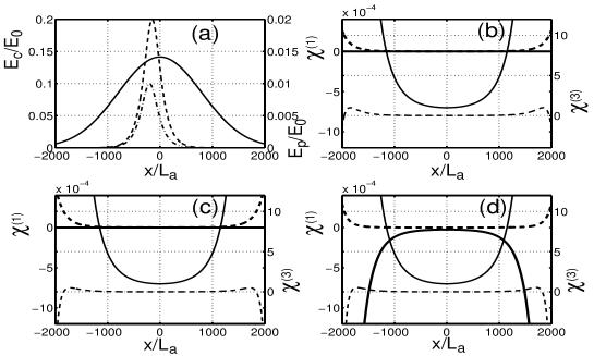
Figure 2: (a) shows the transverse profile of the coupling light beam (solid curve) and the fundamental soliton (dot-dashed curve) or second-order soliton formed by the probe light beam. (b), (c) and (d) show the transverse structures of the coupling-light-induced nonlinear waveguide: linear susceptibility $\chi^{(1)}$ (thick lines) and third-order susceptibilities $\chi^{(3)}$ (thin lines), in which solid lines present the real parts and the dashed lines present the imaginary parts, under different conditions, respectively. $\chi^{(1)}$ is in units of $\mu^{2}n/(\varepsilon_{0}\hbar\gamma)$. $\chi^{(3)}$ is in units of $\mu^{2}n/(\varepsilon_{0}\hbar\gamma E_{0}^{2})$.

The unique features of an EIT medium enable the coupling light beam to induce a very special nonlinear waveguide, which can exert very strong effects on the dynamical behaviors of solitons formed by the probe light beam and hence give rise to new soliton controllabilities. Next, solving Eq.(1) (neglecting the coordinate y) numerically by using the Crank-Nicolson method, we show several typical effects of the nonlinear waveguide on the evolution of (1+1)D solitons in the EIT medium. In the calculation, we use $E_{0}=\gamma\hbar/\mu$, $L_{a}=\sqrt{\varepsilon_{0}\gamma\hbar/(n\mu^{2}k_{p}^{2})}$ and $L_{b}=2\varepsilon_{0}\gamma\hbar/(n\mu^{2}k_{p})$ as units to normalize the amplitudes of the electro-magnetic fields and the spatial coordinates $x$ and $z$, respectively.

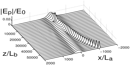
Figure 3: Second-order soliton splits into two solitons under the influence of the transverse variation of the coupling-light-induced nonlinear susceptibility [see Fig. 2 (b)].

Because the coupling light intensity is approximately inversely proportional to the nonlinear susceptibility under the EIT condition, the coupling-light-induced transverse variation of the nonlinear susceptibility can strongly affect the dynamical behaviors of high-order solitons in the EIT medium. For example, the gradient of the real part of the coupling-light-induced third-order susceptibility, as shown by the thin solid curve in Fig. 2 (b), can lead to splitting of a second-order soliton [The maximum amplitude is twice that of the soliton described by Eq. (6)], as shown in Fig.3. In this calculation, we assume that the coupling light beam has a Gaussian profile along the $x$ axis [See the solid curve in Fig.2(a)], and propagates along the z axis with negligible diffraction. Other parameters are as follows: $\Delta_{13}=\Delta_{23}=0\gamma$, $\Delta_{23}=100\gamma$, $\gamma_{2}=1\times 10^{-8}\gamma$. The linear and nonlinear susceptibilities induced by this light beam are shown in Fig.2(b). The initial second-order soliton formed by the probe light beam has a small transverse displacement from the center of the coupling beam, as shown by the dashed line in Fig.2(a), hence it experiences a non-uniform nonlinear phase modulation due to the gradient of the third-order susceptibility. As we known, if a second-order soliton propagates in a uniform Kerr nonlinear medium, it only exhibits periodic oscillation SolitonBooks . The splitting of the second-order soliton into two solitons is therefore just due to the transverse variation of the nonlinear susceptibility. Because the split solitons have opposite transverse momentums, one split soliton propagates into the lower coupling intensity regime, i.e., the larger nonlinearity region; it becomes narrower. The other one propagates to the higher coupling intensity regime, i.e., the smaller nonlinearity region; it becomes wider.

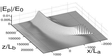
Figure 4: Absorption of the soliton due to the increasing linear absorption at the boundary of the coupling beam.

At the boundary of the coupling beam, the linear absorption due to ground-state dephasing increases very fast. As a result, if a soliton propagates toward the boundary of the coupling beam, its amplitude will decay very quickly because of the absorption, as shown in Fig. 4. In this calculation, we slightly increase the decay rate of the gound state $\left|2\right\rangle$, i.e., $\gamma_{2}=2\times 10^{-8}\gamma$, to make the linear absorption more apparent, as indicated by the imaginary part of the linear susceptibility (thick dashed line) in Fig. 2(c). The initial fundamental soliton with zero transverse velocity has a larger offset from the center of the coupling beam, as plotted by the dot-dashed line in Fig. 2(a). Due to the gradient of the nonlinear susceptibility, the soliton is transversely accelerated and propagates toward the boundary of the coupling beam. Because of the linear absorption becomes larger and larger, the amplitude of the soliton is quickly reduced. However, the width of the soliton becomes smaller in comparison with its initial value, although the amplitude becomes smaller because the nonlinear susceptibility becomes larger relatively more rapidly in this specific condition.

If the detuning $\Delta_{13}$ is finite, the coupling beam can form a high-linear-refractive-index waveguide overlapping with the nonlinear one and force the soliton to oscillate nonlinearly inside the waveguide FocusPRL . For example, we follow the above parameters values except for setting $\Delta_{13}=-5\times 10^{-7}\gamma$, $\gamma_{2}=5\times 10^{-9}\gamma$, and we find that the real part of the linear susceptibility is much reduced at the boundary of the coupling beam [See the thick solid line in Fig. 2(d)]. Thus, the linear susceptibility behaves as a potential, which confines the soliton to oscillate, as shown in Fig. 5. The oscillation is nonlinear because of the nonuniform nonlinear susceptibility. For example, the initial transversely static soliton is accelerated by the gradient of the nonlinear susceptibility because the amplitude of the soliton is very large and the soliton propagates toward the boundary of the coupling beam, as shown in Fig. 5(b). But, because the linear absorption becomes larger and larger, the intensity of the soliton become smaller and smaller. As a result, the acceleration due to the nonlinear susceptibility becomes smaller and smaller. When the acceleration due to the linear susceptibility overcomes the nonlinear one, the soliton is gradually decelerated, and finally reverses its propagation direction and oscillates around the center of the coupling beam.

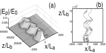
Figure 5: Nonlinear oscillation of the soliton due to the transverse confinement produced by the coupling-light-induced non-uniform linear and nonlinear susceptibilities [See Fig. 2 (d)]. Here (b) is the contour graph of (a).

In conclusion, we have shown a weak probe light beam can form spatial solitons in an electro-magnetically induced transparency medium composed of four-level atoms and a coupling light field. We have found that the coupling light beam can induce a highly controllable nonlinear waveguide and exert very strong effects on the dynamical behaviors of the solitons. Hence, in the EIT medium, it is not only possible to produce spatial solitons at very low light intensities but also simultaneously control these solitons by using the coupling-light-induced nonlinear waveguide.

I thank Makoto Yamashita and Michael Wong Jack for their very helpful discussions.

References

- (1) P. D. Drummond, R. M. Shelby, S. R. Friberg, Y. Yamamoto, Nature (London) 365, 307 (1993); S. R. Friberg, et al., Phys. Rev. Lett. 77, 3775 (1996).
- (2) Yu. S. Kivshar, B. Luther-Davies, Phys. Rept. 298, 81 (1998); G. Stegeman and M. Segev, Science 286, 1518 (1999).
- (3) R. Y. Chiao, I. H. Deutsch, John C. Garrison, Phys. Rev. Lett. 67, 1399 (1991); I. H. Deutsch, et al., ibid. 69, 3627 (1992).
- (4) G. A. Swartzlander, et al., Phys. Rev. Lett. 66, 1583 (1991); V. Tikhonenko, et al., ibid. 76, 2698 (1996).
- (5) S. E. Harris, Phys. Today 50, 36 (1997); E. Arimondo, in Progress in Optics XXXV, edited by E. Wolf (Elsevier, Amsterdam, 1996), p. 257; M. Xiao, et al., Phys. Rev. Lett. 74, 666 (1995); L. V. Hau, et al., Nature (London) 397, 594 (1999); M. M. Kash, et al., Phys. Rev. Lett. 82, G. 5229 (1999); D. Budker, et al., ibid. 83, 1767 (1999).
- (6) S. E. Harris, et al., Phys. Rev. Lett. 64, 1107 (1990); K. Hakuta, et al., ibid. 66, 596 (1991).
- (7) H. Schmidt and A. Imamoglu, Opt. Lett. 21, 1936 (1996).
- (8) H. Wang, D. Goorskey, and M. Xiao, Phys. Rev. Lett. 87, 073601 (2001); H. Wang, et al., Phys. Rev. A 65 011801 (2002); H. Wang, et al., Phys. Rev. A 65, 051802 (2002); H. Wang, et al.,, Opt. Lett. 27, 258 (2002).
- (9) A. Imamoglu, H. Schmidt, G. Woods, and M. Deutsch, Phys. Rev. Lett. 79, 1467 (1997).
- (10) M. D. Lukin and A. Imamoglu, Phys. Rev. Lett. 84, 1419 (2000). M. Fleischhauer and M. D. Lukin, ibid. 84, 5094 (2000); M. D. Lukin, A. Imamoglu, Nature 413, 273 (2001).
- (11) T. Hong, M. W. Jack, M. Yamashita, Takaaki Mukai, Opt. Commun. 214, 341 (2002).
- (12) Richard R. Moseley, Sara Shepherd, David J. Fulton, Bruce D. Sinclair, and Malcolm H. Dunn, Phys. Rev. Lett. 74, 670 (1995); M. Mitsunaga, M. Yamashita and H. Inoue, Phys. Rev. A 62, 013817 (2000).
- (13) T. Hong et al., to be submitted.
- (14) Govind P. Agrawal, Nonlinear Fiber Optics (Academic Press, New York, 1995).
- (15) V. E. Zakharov, A. B. Shabat, Zh. Eksp. Teor. Fiz. 61, 118 (1971) [Sov. Phys. JETP 34, 62 (1972)]; V. E. Zakharov, A. B. Shabat, ibid. 64, 1627 (1973) [Sov. Phys. JETP 37, 823 (1973)].
- (16) Y. Silberberg, Opt. Lett. 15, 1005 (1990).