IISc-CHEP-8/04
quant-ph/0405128
Quantum Random Walks do not need a Coin Toss

Abstract

Classical randomized algorithms use a coin toss instruction to explore different evolutionary branches of a problem. Quantum algorithms, on the other hand, can explore multiple evolutionary branches by mere superposition of states. Discrete quantum random walks, studied in the literature, have nonetheless used both superposition and a quantum coin toss instruction. This is not necessary, and a discrete quantum random walk without a quantum coin toss instruction is defined and analyzed here. Our construction eliminates quantum entanglement from the algorithm, and the results match those obtained with a quantum coin toss instruction.

I Motivation

Random walks are a fundamental ingredient of non-deterministic algorithms motwani , and are used to tackle a wide variety of problems—from graph structures to Monte Carlo samplings. Such algorithms have many branches, which are explored probabilistically, to estimate the correct result. A classical computer can explore only one branch at a time, so typically the algorithm is executed several times, and the estimate of the final result is extracted from the ensemble of individual executions by methods of probability theory. To ensure that different branches are explored in different executions, one needs non-deterministic instructions, and they are provided in the form of random numbers. A coin toss is the simplest example of a random number generator, and it can be included as an instruction for a probabilistic Turing machine.

A quantum computer can explore multiple branches in a different manner, i.e. by using a superposition of states. The probabilistic result can then be arrived at by interference of amplitudes corresponding to different branches. Thus as long as the means to construct a variety of superposed states exist, there is no a priori reason to include a coin toss as an instruction for a (probabilistic) quantum Turing machine. This is obvious enough, and indeed continuous time quantum random walks have been studied without recourse to a coin toss instruction farhi . Nevertheless, a coin toss instruction has been considered necessary in construction of discrete time quantum random walks (see for instance, Refs.kempe ; ambainis ). In this article, we demonstrate that this is a misconception arising out of unnecessarily restrictive assumptions. We explicitly construct a quantum random walk on a line without using a coin toss instruction, and analyze its properties.

There also exists confusion in the literature about different scaling behavior of discrete and continuous time quantum random walk algorithms (see again, Refs.kempe ; ambainis ), because the former have been constructed using a coin toss instruction while the latter do not contain a coin toss instruction. Our work eliminates this confusion in the sense that scaling behavior of discrete and continuous time quantum random walk algorithms, both constructed without a coin toss instruction, would coincide. Thereafter, a quantum coin would be an additional resource; if its inclusion can improve scaling behavior of some quantum algorithms, that should not be a surprise.

II Quantum Random Walk on a Line

A random walk is a diffusion process, which is generated by the Laplacian operator in the continuum. To construct a discrete quantum walk, we must discretize this process using evolution operators that are both unitary and ultra-local (an ultra-local operator vanishes outside a finite range ultra ). To begin with, consider the walk on a line. The allowed positions are labeled by integers, and the simplest translation invariant ultra-local discretization of the Laplacian operator is

$$H|n\rangle~{}\propto~{}\big{[}-|n-1\rangle+2|n\rangle-|n+1\rangle\big{]}~{}.$$ (1)

The corresponding evolution operator is

$$U(\Delta t)~{}=~{}\exp(iH\Delta t)~{}=~{}1+iH\Delta t+O((\Delta t)^{2})~{}.$$ (2)

With a finite $\Delta t$, $U$ has an exponential tail and so it is not ultra-local. The evolution operator can be made ultra-local by truncation, say by dropping the $O((\Delta t)^{2})$ part, but then it is not unitary. One may search for ultra-local translationally invariant unitary evolution operators using the ansatz

$$U|n\rangle~{}=~{}a|n-1\rangle+b|n\rangle+c|n+1\rangle~{},$$ (3)

but then the orthogonality constraints between different rows of the unitary matrix make two of $\{a,b,c\}$ vanish, and one obtains a directed walk instead of a random walk.

One way to bypass this problem and construct a ultra-local unitary random walk is to enlarge the Hilbert space and add a quantum coin toss instruction, e.g.

$$U=\sum_{n}\Big{[}|\!\uparrow\rangle\langle\uparrow\!|\otimes|n+1\rangle\langle n|+|\!\downarrow\rangle\langle\downarrow\!|\otimes|n-1\rangle\langle n|\Big{]}.$$ (4)

This modification however brings its own set of caveats. If the coin state is measured at every time step (in other words, if the coin is classical), one gets no improvement over the classical random walk. With a unitary coin evolution operator, that entangles the coin state with the position state, the quantum walk performs better than the classical walk in certain algorithms. But in this case, the final results depend on the initial state of the coin, because quantum evolution is reversible and not Markovian. For example, the final state distribution of the quantum walk depends on whether the initial coin state was $|\!\uparrow\rangle$, or $|\!\downarrow\rangle$, or some linear combination thereof. To get around this initial coin state sensitivity, further algorithmic modifications such as averaging over initial coin states, or intermittent coin measurements, or use of multiple coins, have been suggested, but they still leave a feeling of something to be desired.

II.1 Getting Rid of the Coin

The way out of the above conundrum is familiar to lattice field theorists staggered . It has also been used to simulate quantum scattering with ultra-local operators richardson , and to construct quantum cellular automata meyer . In its simplest version, the Laplacian operator is decomposed into its even/odd parts, $H=H_{e}+H_{o}$,

$$H\propto\left(\matrix{\cdots&\cdots&\cdots&\cdots&\cdots&\cdots&\cdots&\cdots\cr\cdots&\hfill-1&\hfill 2&\hfill-1&\hfill 0&\hfill 0&\hfill 0&\cdots\cr\cdots&\hfill 0&\hfill-1&\hfill 2&\hfill-1&\hfill 0&\hfill 0&\cdots\cr\cdots&\hfill 0&\hfill 0&\hfill-1&\hfill 2&\hfill-1&\hfill 0&\cdots\cr\cdots&\hfill 0&\hfill 0&\hfill 0&\hfill-1&\hfill 2&\hfill-1&\cdots\cr\cdots&\cdots&\cdots&\cdots&\cdots&\cdots&\cdots&\cdots\cr}\right),$$ (5)

$$H_{e}\propto\left(\matrix{\cdots&\cdots&\cdots&\cdots&\cdots&\cdots&\cdots&\cdots\cr\cdots&\hfill-1&\hfill 1&\hfill 0&\hfill 0&\hfill 0&\hfill 0&\cdots\cr\cdots&\hfill 0&\hfill 0&\hfill 1&\hfill-1&\hfill 0&\hfill 0&\cdots\cr\cdots&\hfill 0&\hfill 0&\hfill-1&\hfill 1&\hfill 0&\hfill 0&\cdots\cr\cdots&\hfill 0&\hfill 0&\hfill 0&\hfill 0&\hfill 1&\hfill-1&\cdots\cr\cdots&\cdots&\cdots&\cdots&\cdots&\cdots&\cdots&\cdots\cr}\right),$$ (6)

$$H_{o}\propto\left(\matrix{\cdots&\cdots&\cdots&\cdots&\cdots&\cdots&\cdots&\cdots\cr\cdots&\hfill 0&\hfill 1&\hfill-1&\hfill 0&\hfill 0&\hfill 0&\cdots\cr\cdots&\hfill 0&\hfill-1&\hfill 1&\hfill 0&\hfill 0&\hfill 0&\cdots\cr\cdots&\hfill 0&\hfill 0&\hfill 0&\hfill 1&\hfill-1&\hfill 0&\cdots\cr\cdots&\hfill 0&\hfill 0&\hfill 0&\hfill-1&\hfill 1&\hfill 0&\cdots\cr\cdots&\cdots&\cdots&\cdots&\cdots&\cdots&\cdots&\cdots\cr}\right).$$ (7)

The two parts, $H_{e}$ and $H_{o}$, are individually Hermitian. They are block-diagonal with a constant $2\times 2$ matrix, and so they can be exponentiated while maintaining ultra-locality. The total evolution operator can therefore be easily truncated, without giving up either unitarity or ultra-locality,

$$U(\Delta t)=e^{i(H_{e}+H_{o})\Delta t} = e^{iH_{e}\Delta t}e^{iH_{o}\Delta t}+O((\Delta t)^{2})$$

$$= U_{e}(\Delta t)U_{o}(\Delta t)+O((\Delta t)^{2})~{}.$$

The quantum random walk can now be generated using $U_{e}U_{o}$ as the evolution operator for the amplitude distribution $\psi(n,t)$,

$$\psi(n,t)=[U_{e}U_{o}]^{t}\psi(n,0)~{},$$ (9)

The fact that $U_{e}$ and $U_{o}$ do not commute with each other is enough for the quantum random walk to explore all possible states. The price paid for the above manipulation is that the evolution operator is translationally invariant along the line in steps of 2, instead of 1.

The $2\times 2$ matrix appearing in $H_{e}$ and $H_{o}$ is proportional to $(1-\sigma_{1})$, and so its exponential will be of the form $(c1+is\sigma_{1})$, $|c|^{2}+|s|^{2}=1$. A random walk should have at least two non-zero entries in each row of the evolution operator. Even though our random walk treats even and odd sites differently by construction, we can obtain an unbiased random walk, by choosing the $2\times 2$ blocks of $U_{e}$ and $U_{o}$ as $\frac{1}{\sqrt{2}}{1\,i\choose i\,1}$. The discrete quantum random walk then evolves the amplitude distribution according to

$$U_{o}|n\rangle = {1\over\sqrt{2}}\Big{[}|n\rangle+i|n+(-1)^{n}\rangle\Big{]},$$ (10)

$$U_{e}|n\rangle = {1\over\sqrt{2}}\Big{[}|n\rangle+i|n-(-1)^{n}\rangle\Big{]},$$ (11)

$$U_{e}U_{o}|n\rangle={1\over 2}\Big{[}i|n-1\rangle+|n\rangle+i|n+1\rangle-|n+2(-1)^{n}\rangle\Big{]}.$$ (12)

II.2 Relation to the Walk with a Coin

Our construction of discrete quantum random walk has exchanged the up/down coin states for the even/odd site label. In the language of lattice field theory, this strategy resembles staggered fermions staggered , while that with a coin (or spin) is akin to Wilson fermions wilson . Indeed, an explicit relation between our construction and that with a coin can be established. Let

$$\Psi(n,t)\equiv\left(\matrix{\psi(2n,t)\cr\psi(2n+1,t)\cr}\right)$$ (13)

describe the amplitude distribution in a two-component notation. Then Eqs.(9,12) are equivalent to the evolution

$$\Psi(N,t)=[UC]^{t}\Psi(N,0)~{},~{}~{}C={1\over\sqrt{2}}\left(\matrix{1&i\cr i&1\cr}\right)~{},$$ (14)

$$U|N\rangle={1\over\sqrt{2}}|N\rangle+{i\sigma_{1}\over\sqrt{2}}\sum_{\pm}{1\pm\sigma_{3}\over 2}|N\mp 1\rangle~{}.$$ (15)

Here, for clarity, we have denoted the basis states for $\Psi$ by $|N\rangle$. The symmetric coin operator $C$ mixes the up/down components of $\Psi$. The walk operator $U$ distributes the amplitude equally between remaining at the same site and moving to the neighboring sites. The projection operators $(1\pm\sigma_{3})/2$ pick out the amplitude components that move forward and backward. Finally, the operator $\sigma_{1}$ interchanges the up/down components of $\Psi$, producing what Ref.gridsrch1 has called the flip-flop walk.

It is also instructive to note that while the diffusion operator $H$ has the structure of a second derivative, its two parts, $H_{e}$ and $H_{o}$, have the structure of a first derivative. This split is reminiscent of the “square-root” one takes to go from the Klein-Gordon operator to the Dirac operator. For a quantum random walk with a coin, this feature has been used to construct an efficient search algorithm on a spatial lattice of dimension greater than one gridsrch1 ; gridsrch2 . Reanalysis of that problem is in progress, without using a coin, in view of our results inprogress .

III Analysis of the Walk

It is straightforward to analyze the properties of the walk in Eq.(12) using the Fourier transform:

$$\widetilde{\psi}(k,t)=\sum_{n}e^{ikn}\psi(n,t)~{},~{}$$ (16)

$$\psi(n,t)=\int_{-\pi}^{\pi}{dk\over 2\pi}~{}e^{-ikn}\widetilde{\psi}(k,t)~{}.$$ (17)

The evolution of the amplitude distribution in Fourier space is easily obtained by splitting it into its even/odd parts:

$$\psi\equiv\left(\matrix{\psi_{e}\cr\psi_{o}\cr}\right)~{},~{}~{}\psi(k,t)=[M(k)]^{t}\psi(k,0)~{},~{}$$ (18)

$$M(k)=\left(\matrix{-ie^{ik}\sin k&i\cos k\cr i\cos k&ie^{-ik}\sin k\cr}\right)~{}.$$ (19)

The unitary matrix $M$ has the eigenvalues, $\lambda_{\pm}\equiv e^{\pm i\omega_{k}}$ (this $\pm$ sign label continues in all the results below),

$$\lambda_{\pm}=\sin^{2}k\pm i\cos k\sqrt{1+\sin^{2}k}~{},~{}~{}\omega_{k}=\cos^{-1}(\sin^{2}k)~{},$$ (20)

with the (unnormalized) eigenvectors,

$$e_{\pm} \propto \left(\matrix{-\sin k\pm\sqrt{1+\sin^{2}k}\cr 1\cr}\right)~{},$$ (21)

$$\propto \left(\matrix{1\cr\sin k\pm\sqrt{1+\sin^{2}k}\cr}\right)~{}.$$

The evolution of amplitude distribution then follows

$$\widetilde{\psi}(k,t)=e^{iw_{k}t}\widetilde{\psi}_{+}(k,0)+e^{-iw_{k}t}\widetilde{\psi}_{-}(k,0)~{},$$ (22)

where $\widetilde{\psi}_{\pm}(k,0)$ are the projections of the initial amplitude distribution along $e_{\pm}$. The amplitude distribution in the position space is given by the inverse Fourier transform of $\widetilde{\psi}(k,t)$. While we are unable to evaluate it exactly, many properties of the quantum random walk can be extracted numerically as well as by suitable approximations.

Consider a walk starting at the origin, $\psi_{\rm o}(n,0)=\delta_{n,0}$. Its amplitude distribution at later times is specified by

$$\widetilde{\psi}_{{\rm o},\pm}(k,0)={\pm 1\over 2\sqrt{1+\sin^{2}k}}\left(\matrix{-\sin k\pm\sqrt{1+\sin^{2}k}\cr 1\cr}\right)~{},$$ (23)

$$\psi_{\rm o}(n,t) = {1\over 2\pi}\int_{-\pi}^{\pi}{dk~{}e^{-ikn}\over\sqrt{1+\sin^{2}k}}$$

$$\times \left(\matrix{-i\sin\omega_{k}t\sin k+\cos\omega_{k}t\sqrt{1+\sin^{2}k}\cr i\sin\omega_{k}t\cr}\right)~{}.$$

This walk is asymmetric because our definitions treat even and odd sites differently. We can get rid of the asymmetry by initializing the walk as $\psi_{\rm s}(n,0)=(\delta_{n,0}+\delta_{n,1})/\sqrt{2}$. The walk is then symmetric under $n\leftrightarrow(1-n)$, and the amplitude distribution evolves according to

$$\widetilde{\psi}_{{\rm s},\pm}(k,0) = {\pm 1\over 2\sqrt{2(1+\sin^{2}k)}}$$

$$\times \left(\matrix{e^{ik}-\sin k\pm\sqrt{1+\sin^{2}k}\cr 1+e^{ik}\sin k\pm e^{ik}\sqrt{1+\sin^{2}k}\cr}\right)~{},$$

$$\psi_{\rm s}(n,t)={1\over 2\pi}\int_{-\pi}^{\pi}{dk~{}e^{-ikn}\over\sqrt{2(1+\sin^{2}k)}}$$

$$\times \left(\matrix{i\sin\omega_{k}t(e^{ik}-\sin k)+\cos\omega_{k}t\sqrt{1+\sin^{2}k}\cr i\sin\omega_{k}t(1+e^{ik}\sin k)+\cos\omega_{k}t~{}e^{ik}\sqrt{1+\sin^{2}k}\cr}\right)~{}.$$

Figs.1-2 show the numerically evaluated probability distributions, after $32$ time steps, for asymmetric and symmetric quantum random walks respectively. Note that, by construction, the distributions after $t$ time steps remain within the interval $[-2t+1,2t]$.

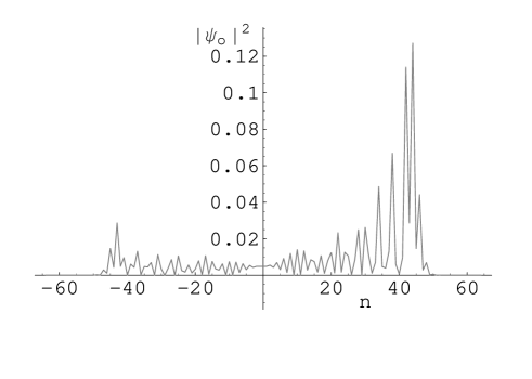
Figure 1: Probability distribution after $32$ time steps for the asymmetric quantum random walk $\psi_{\rm o}$.

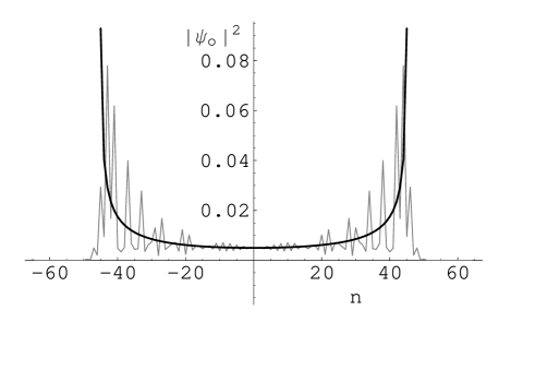
Figure 2: Probability distribution after $32$ time steps for the symmetric quantum random walk $\psi_{\rm s}$. The dark curve denotes the smoothed distribution of Eq.(39).

III.1 Asymptotic Behavior of the Walk

For large $t$, a good approximation to the distribution, Eq.(III), can be obtained by the stationary phase method, as in Ref.nayak . The integral is periodic, and a sum of terms of the form

$$I(n,t)=\int_{\pi}^{\pi}{dk\over 2\pi}~{}g(k)~{}e^{i\phi(k,n,t)}~{}.$$ (27)

The highly oscillatory part of the integrand is determined by $\phi(k,n,t)=-kn\pm\omega_{k}t$, while the remaining part $g(k)$ is bounded. Simple algebra yields

$${d\omega_{k}\over dk} = -{2\sin k\over\sqrt{1+\sin^{2}k}}~{},$$ (28)

$${d^{2}\omega_{k}\over dk^{2}} = -{2\cos k\over(1+\sin^{2}k)^{3/2}}~{},$$ (29)

$${d^{3}\omega_{k}\over dk^{3}} = {4\sin k(1+\cos^{2}k)\over(1+\sin^{2}k)^{5/2}}~{}.$$ (30)

The stationary point of the integral, $k=k_{0}$, has to satisfy

$$\alpha\equiv{n\over t}=\mp{2\sin k_{0}\over\sqrt{1+\sin^{2}k_{0}}}~{},$$ (31)

which has a solution only for $n\in[-\sqrt{2}t,\sqrt{2}t]$.

We now separately consider the three cases:
(1) $|n|>\sqrt{2}t$: There is no stationary point in this case. For $|n|=(\sqrt{2}+\epsilon)t$, $|d\phi(k)/dk|>\epsilon$, and repeated integration by parts shows that the integral falls off faster than any positive integer power of $\epsilon t$.
(2) $|n|=\sqrt{2}t$: In this case, there is a stationary point of order 2 at $k_{0}=\mp{\rm sgn}(n){\pi/2}$. The integral is therefore proportional to $t^{-1/3}$. Explicitly,

$$\psi_{\rm s}(\sqrt{2}t,t) = c~{}t^{-1/3}\left(\matrix{(1+{1-i\over\sqrt{2}})\cos({\pi t\over\sqrt{2}})\cr(1-{1-i\over\sqrt{2}})\sin({\pi t\over\sqrt{2}})\cr}\right),$$ (32)

$$\psi_{\rm s}(-\sqrt{2}t,t) = c~{}t^{-1/3}\left(\matrix{(1-{1-i\over\sqrt{2}})\cos({\pi t\over\sqrt{2}})\cr(-1-{1-i\over\sqrt{2}})\sin({\pi t\over\sqrt{2}})\cr}\right),$$ (33)

$$c = {1\over 2\pi 3^{1/6}}~{}\Gamma\left({1\over 3}\right)\approx 0.355~{}.$$ (34)

(3) $|n|<\sqrt{2}t$: There are two stationary points in this case, $k_{01}\in(-\pi/2,\pi/2)$ and $k_{02}=\pi-k_{01}$, with

$$\sin k_{0} = \mp{n\over\sqrt{4t^{2}-n^{2}}}~{},~{}$$ (35)

$$\left|{d^{2}\omega_{k}\over dk^{2}}\right|_{k=k_{0}} = {\sqrt{4t^{2}-2n^{2}}~{}(4t^{2}-n^{2})\over 4t^{3}}~{}.$$ (36)

The integral is therefore proportional to $t^{-1/2}$. In terms of the phase,

$$\phi_{0}=-k_{01}n+\omega_{k_{0}}t-(\pi/4)~{},$$ (37)

the distribution amplitude is

$$\psi_{\rm s} = {1\over\sqrt{t}(4t^{2}-2n^{2})^{1/4}}$$

$$\times \left[\cos\phi_{0}\left(\matrix{((1-i)n+2t)/\sqrt{4t^{2}-n^{2}}\cr\sqrt{4t^{2}-2n^{2}}/(2t+n)\cr}\right)\right.$$

$$\left.+i\sin\phi_{0}\left(\matrix{\sqrt{4t^{2}-2n^{2}}/\sqrt{4t^{2}-n^{2}}\cr((1-i)n+2t)/(2t+n)\cr}\right)\right]~{}.$$

The smoothed probability distribution, obtained by replacing the highly oscillatory terms by their mean values, is

$$|\psi_{\rm s}|_{\rm smooth}^{2}={4t^{2}\over\pi\sqrt{4t^{2}-2n^{2}}~{}(4t^{2}-n^{2})}~{}.$$ (39)

(Here, the $n\leftrightarrow(1-n)$ symmetry can be restored by replacing $n$ by $(n-{1\over 2})$.) As shown in Fig.2, it represents the average behavior of the distribution very well. Its low order moments are easily calculated to be,

$$\int_{n=-\sqrt{2}t}^{\sqrt{2}t}|\psi_{\rm s}|_{\rm smooth}^{2}dn = 1~{},$$ (40)

$$\int_{n=-\sqrt{2}t}^{\sqrt{2}t}|n|\cdot|\psi_{\rm s}|_{\rm smooth}^{2}dn = t~{},$$ (41)

$$\int_{n=-\sqrt{2}t}^{\sqrt{2}t}n^{2}|\psi_{\rm s}|_{\rm smooth}^{2}dn = 2(2-\sqrt{2})t^{2}~{}.$$ (42)

The following properties of the quantum random walk are easily deduced from all the above results:
$\bullet$ The probability distribution is double-peaked with maxima approximately at $\pm\sqrt{2}t$. The distribution falls off steeply beyond the peaks, while it is rather flat in the region between the peaks. With increasing $t$, the peaks become more pronounced, because the height of the peaks decreases slower than that for the flat region.
$\bullet$ The size of the tail of the amplitude distribution is limited by $(\epsilon t)^{-1}\sim t^{-1/3}$, which gives $\Delta n_{>}=\Delta(\epsilon t)=O(t^{1/3})$. On the inner side, the width of the peaks is governed by $|\omega_{k}^{{}^{\prime\prime}}t|^{-1/2}\sim t^{-1/3}$. For $|n|=(\sqrt{2}-\delta)t$, this gives $\Delta n_{<}=\Delta(\delta t)=O(t^{1/3})$. The peaks therefore make a negligible contribution to the probability distribution, $O(t^{-1/3})$.
$\bullet$ Rapid oscillations contribute to the probability distribution (and hence to its moments) only at subleading order. They can be safely ignored in an asymptotic analysis, retaining only the smooth part of the probability distribution.
$\bullet$ The quantum random walk spreads linearly in time, with a speed smaller by a factor of $\sqrt{2}$ compared to a directed walk. This speed is a measure of its mixing behavior and hitting probability. The probability distribution is qualitatively similar to a uniform distribution over the interval $[-\sqrt{2}t,\sqrt{2}t]$. In particular, $m^{th}$ moment of the probability distribution is proportional to $t^{m}$.

These properties agree with those obtained in Ref.nayak for a quantum random walk with a coin-toss instruction, demonstrating that the coin offers no advantage in this particular set up. (Extra factors of $2$ appear in our results, because a single step of our walk is a product of two nearest neighbor operators, $U_{e}$ and $U_{o}$.) It is important to note that the properties of the quantum random walk are in sharp contrast to those of the classical random walk. The classical random walk produces a binomial probability distribution, which in the symmetric case has a single peak centered at the origin and variance equal to $t$.

III.2 The Walk in Presence of an Absorbing Wall

The escape probability of the quantum random walk can be calculated by introducing an absorbing wall, say between $n=0$ and $n=-1$. Mathematically, the absorbing wall can be represented by a projection operator for $n\geq 0$. The unabsorbed part of the walk is given by

$$\psi(n,t+1) = P_{n\geq 0}U_{e}U_{o}~{}\psi(n,t)~{},$$

$$= U_{e}U_{o}~{}\psi(n,t)-{1\over 2}\delta_{n,-1}(i\psi(0,t)-\psi(1,t))~{},$$

with the absorption probability,

$$P_{\rm abs}(t)=1-\sum_{n\geq 0}|\psi(n,t)|^{2}~{}.$$ (44)

Fig.3 shows the numerically evaluated probability distribution, in presence of this absorbing wall, after $32$ time steps and with the symmetric initial state. Comparison with Fig.2 shows that the absorbing wall disturbs the evolution of the walk only marginally. The probability distribution in the region close to $n=0$ is depleted as anticipated, while it is a bit of a surprise that the peak height near $n=\sqrt{2}t$ increases slightly. As a result, the escape speed from the wall is little higher than the spreading speed without the wall. As shown in Fig.4, we find that the first two time steps dominate absorption, $P_{\rm s,abs}(t=1)=0.25$ and $P_{\rm s,abs}(t=2)=0.375$, with very little absorption later on. Asymptotically, the net absorption probability approaches $P_{\rm s,abs}(\infty)\approx 0.4098$ for the symmetric walk. (We also find, for the asymmetric walk starting at the origin, $P_{\rm o,abs}(\infty)\approx 0.2732$.) This value is smaller than the corresponding result $P_{\rm abs}(\infty)=2/\pi$ for the symmetric quantum random walk with a coin-toss instruction watrous .

Thus the part of quantum random walk going away from the absorbing wall just takes off at a constant speed, hardly ever returning to the starting point. Again, this behavior is in a sharp contrast to that of the classical random walk. A classical random walk always returns to the starting point, sooner or later, and so its absorption probability approaches unity as $t\rightarrow\infty$.

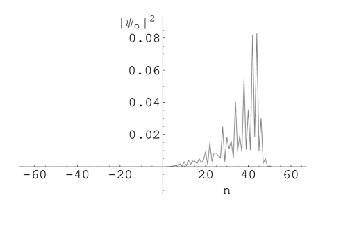
Figure 3: Probability distribution after $32$ time steps for the symmetric quantum random walk, with an absorbing wall on the left side of $n=0$.

Figure 4: Time dependence of the probability for the symmetric quantum random walk to remain unabsorbed, in presence of an absorbing wall to the left of $n=0$. The walk gets within a few per cent of the asymptotic escape probability in just two time steps.

III.3 Comparison to the Walk with a Coin

The above results bring out the differences of our quantum random walk construction compared to that of Refs.nayak ; watrous :
(1) We have absorbed the two states of the coin in to the even/odd site label at no extra cost. This is possible because, due to its discrete symmetry, the walk with a coin effectively uses only half the sites (e.g. for a walk starting at origin, the amplitude distribution is restricted to only odd sites at odd $t$ and only even sites at even $t$). Our walk makes use of all the sites at every instance.
(2) It can be seen from Eqs.(15,4) that, at every time step, $\Psi$ has 50% probability to stay put at the same location, while the walk with a coin has no probability to remain at the same location. Yet, both achieve the same spread of amplitude distribution, as exemplified by the moments in Eqs.(40-42). This means that our walk is smoother—more directed and less zigzag.
(3) When the coin is considered a separate degree of freedom, quantum evolution entangles the coin and the walk position. On the other hand, when the coin states are made part of the position space, as we have done, entanglement disappears completely—only superposition representing the amplitude distribution survives entangle . This elimination of quantum entanglement would be a tremendous advantage in any practical implementation of the quantum random walk, because quantum entanglement is highly fragile against environmental disturbances while mere superposition is much more stable. The cost for gaining this advantage is the loss of short distance homogeneity—translational invariance holds in steps of 2 instead of 1.

IV Extensions and Outlook

The quantum random walk on a line is easily converted to that on a circle by imposing periodic boundary conditions. When the circle has $N$ points, the only change in the analysis is to replace the integral over $k$ in the inverse Fourier transform by a discrete sum over $k$-values separated by $2\pi/N$. Since the quantum random walk spreads essentially uniformly, there is not much change in its behavior. All that one has to bear in mind is that, on a long time scale, unitary evolution makes the walk cycle through phases of spreading out and contracting towards the initial state.

Going beyond one dimension, the strategy of constructing discrete ultra-local unitary evolution operators by splitting the Hamiltonian in to block-diagonal parts is applicable to random walks on any finite-color graph richardson . One just constructs $2\times 2$ block unitary matrices for each color of the graph, and the single time step evolution operator becomes the product of all the block unitary matrices. In particular, the $d-$dimensional hypercubic walk can be constructed as a tensor product of $d$ one-dimensional walks, using $2d$ block unitary matrices.

Our results clearly demonstrate that discrete quantum random walks with useful properties can be constructed without a coin toss instruction. The addition of a coin toss instruction may still be beneficial in specific quantum problems. A coin is an extra resource, and there are known instances where the addition of a coin toss instruction makes classical randomized algorithms have a better scaling behavior compared to their deterministic counterparts motwani . One may hope for a similar situation in the quantum case too, keeping in mind that a careful initialization of the quantum coin state would be a must in such cases.

A clear advantage of quantum random walks is their linear spread in time, compared to square-root spread in time for classical random walks. So they are expected to be useful in problems requiring fast hitting times. Some examples of this nature have been explored in graph theoretical and sampling problems (see Refs.kempe ; ambainis for reviews), and more applications need to be investigated.

References

- (1) R. Motwani and P. Raghavan, Randomized Algorithms, Cambridge Univ. Press (1995).
- (2) E. Farhi and S. Gutmann, Phys. Rev. A 58 (1998) 915, quant-ph/9706062.
- (3) J. Kempe, Contemporary Physics 44 (2003) 307, quant-ph/0303081.
- (4) A. Ambainis, quant-ph/0403120.
- (5) We deliberately use the label “ultra-local” here, because ”local” physical interactions (especially when described in the renormalization group framework) include all those that fall off exponentially or faster with distance.
- (6) L. Susskind, Phys. Rev. D 16 (1977) 3031.
- (7) J.L. Richardson, Computer Physics Comm. 63 (1991) 84.
- (8) D.A. Meyer, J. Stat. Phys. 85 (1996) 551.
- (9) K. Wilson, in New Phenomena in Subnuclear Physics, A. Zichichi (ed.), Plenum Press (1977).
- (10) A. Ambainis, J. Kempe and A. Rivosh, quant-ph/0402107.
- (11) A.M. Childs and J. Goldstone, Phys. Rev. A 70 (2004) 042312, quant-ph/0405120.
- (12) A. Patel, K.S. Raghunathan and P. Rungta, in preparation.
- (13) A. Nayak and A. Vishwanath, quant-ph/0010117.
- (14) A. Ambainis, E. Bach, A. Nayak, A. Vishwanath and J. Watrous, Proceedings of STOC’01 (2001), p.37.
- (15) Entanglement is always defined with respect to a specific division of the whole system in to its parts. If the division scheme is altered, entanglement can change.