I hereby declare that I am the sole author of this thesis.

I authorize the University of Waterloo to lend this thesis to other institutions or individuals for the purpose of scholarly research.

Marcus Silva

I authorize the University of Waterloo to reproduce this thesis by photocopying or other means, in total or in part, at the request of other institutions or individuals for the purpose of scholarly research.

Marcus Silva

The University of Waterloo requires the signatures of all persons using or photocopying this thesis. Please sign below, and give address and date.

Acknowledgments

First and foremost, I thank my parents, Luis and Carol, for everything.

Working at the IQC in Waterloo has been a great opportunity, and I have made many friends from whom I have learned a lot. I must thank Michele Mosca, Christof Zalka, and Martin Rötteler for their support, patience, time, encouragement, and insight; Raymond Laflamme for the encouragement and support; and Wendy Reibel for all the help. I also thank Daniel Gottesman and Achim Kempf, for their interest in my research and their kind agreement to serve on my committee, along with Michele Mosca, Christof Zalka, Raymond Laflamme and Martin Rötteler.

My close friends Laura, Robbi, Ben, my distant friends Ying and Lu, and all other friends in between who helped me unwind when I needed to, should be thanking me for being their friend.

Most importantly, I thank Wenting, for her patience.

Using an error models motivated by the Knill, Laflamme, Milburn proposal for efficient linear optics quantum computing [Nature 409,46–52, 2001], error rate thresholds for erasure errors caused by imperfect photon detectors using a 7 qubit code are derived and verified through simulation. A novel method – based on a Markov chain description of the erasure correction procedure – is developed and used to calculate the recursion relation describing the error rate at different encoding levels from which the threshold is derived, matching threshold predictions by Knill, Laflamme and Milburn [quant-ph/0006120, 2000]. In particular, the erasure threshold for gate failure rate in the same order as the measurement failure rate is found to be above $1.78\%$.

Chapter 1 Introduction

Quantum computation was born when Benioff [2] proposed using the laws of quantum mechanics instead of classical mechanics to perform computation. More importantly for physicists, Feynman [6] pointed out, was the possibility of simulating quantum system by using such quantum computers – because the state space of quantum systems has dimensions that grow exponentially with the number of subsystems involved, they are notoriously inefficient to simulate with classical computers.

Much progress has been done on how to perform certain algorithms much more efficiently in quantum computers, as well as how to simulate quantum systems with quantum computers. The main challenge is to construct physical systems on which such computers may be built. Many proposals have been put forth, each with its strengths and weaknesses, but the recent proposal by Knill, Laflamme and Milburn [18], which uses only linear optics elements and single photon sources and detectors, is of particular interest for various reasons. First of all, it was believed that it was impossible to build a universal quantum computer from linear optics elements because photons do not interact with each other. This proposal relies heavily on state preparation in order to avoid such a hurdle. Moreover, one of the most successful applications of quantum computing, quantum key distribution, would benefit directly from the construction of an optical quantum computer because most protocols are implemented with optical communication. Quantum computation with non-linear optics, on the other hand, is notorious for the photon loss, making it extremely inefficient.

The main problem in a physical implementation of a quantum computer is its sensitivity to error and to the environment. In a classical computer, information is represented by two different states, $\mathfrak{0}$ and $\mathfrak{1}$, and such computers can easily be built so that error in distinguishing between these two states is insignificant. In a quantum computer, the state may be in a superposition of these two basis states, say $\alpha\left|{\mathfrak{0}}\right\rangle+\beta\left|{\mathfrak{1}}\right\rangle$, and when the state is measured, we obtain $\left|{\mathfrak{0}}\right\rangle$ with probability $|\alpha|^{2}$, and $\left|{\mathfrak{1}}\right\rangle$ with probability $|\beta|^{2}$. The information in a quantum computer ends up being more akin to an analog data than to digital data, even though there is only a discrete number of basis states. Imprecision in devices used for computation, the logic gates, has a much greater impact in quantum information than in classical information. Moreover, it is much harder to isolate a quantum system from the environment, so that interaction between the two also end up introducing error into the computation, in an effect known as decoherence, which is only observed in quantum systems.

The linear optics quantum computing proposal also suffers from these problems, even though photons are much less sensitive to decoherence than other physical systems proposed for quantum computation. The reason is that the gates proposed for efficient linear optics quantum computation are probabilistic, so that even with infinite precision in the linear optics elements, they may fail. The authors of the proposal have demonstrated that by encoding the data carefully, one can easily overcome the probabilistic nature of the gates [17]. However, these gates depend on single photon measurements, which are known to have low efficiency, although the gates described in the proposal can flag when detectors have failed and replace the lost qubit automatically. The natural question then is what is the maximum rate at which photons may be lost in these gates while still allowing for scalable quantum computation? The main objective of this thesis is to answer that question.

This thesis is organized as follows. Chapter 2 gives a basic overview of quantum erasure correction codes and fault-tolerant computation, focusing on CSS codes and the stabilizer formalism. Chapter 3 describes the basics of the efficient linear optics quantum computation proposal by Knill, Laflamme and Milburn, focusing on the description of the error model for teleportation failures due to the inherent probabilistic nature of the linear optics implementation, as well as photon loss due to detector inefficiencies. Chapter 4 gives a detailed description of the Steane code, and contrasts it to the Grassl code in the context of the error model for linear optics quantum computing. Given these background chapters, it becomes clear how to perform the erasure correction procedure, and in Chapter 5 a new and compact description of the procedure is given in terms of Markov chains. With this description the threshold is obtained for both error models, with the detailed calculations being presented in the appendices. In Chapter 6 a Monte Carlo simulation of the erasure correction procedure is described, and the simulation results are presented and contrasted with the theoretical prediction of Chapter 5. The thesis concludes with a discussion of the results, and suggestions for future work.

1.1 Notation

Some basic notation is assumed in this thesis, and it is briefly reviewed here. Other notation is introduced in the body of the thesis as needed, along with explanations.

In order to emphasize the difference between qubits and photon number states, qubits in the computational basis will be represented with gothic font, e.g. $\left|{\mathfrak{0}}\right\rangle$ and $\left|{\mathfrak{1}}\right\rangle$, while photon numbers will be represented in the usual fonts, e.g. $\left|{1}\right\rangle$ and $\left|{2}\right\rangle$. Operators acting on the physical qubits (qubits not encoded by error correction code) are denoted by bold capital letters, e.g. ${\bf X}$, and multi-letter operators use typewriter font, e.g. ${\tt CNOT}$. Operators acting on the encoded qubits are denoted in the same way, with an added overbar, e.g. $\overline{{\bf X}}$, and encoded qubits also have an overbar, e.g. $\left|{\overline{\Psi}}\right\rangle$ or $\left|{\overline{\mathfrak{01}}}\right\rangle$. If it is clear from the context that the operator is encoded, the overbar is omitted.

The single qubit Pauli group ${\mathcal{P}}_{1}\equiv{\mathcal{P}}$ consists of the operators

$${\bf I} = \begin{pmatrix}1&0\\ 0&1\end{pmatrix}$$ (1.1)

$${\bf X} = \begin{pmatrix}0&1\\ 1&0\end{pmatrix}$$ (1.2)

$${\bf Y} = \begin{pmatrix}0&-1\\ 1&0\end{pmatrix}$$ (1.3)

$${\bf Z} = \begin{pmatrix}1&0\\ 0&-1\end{pmatrix},$$ (1.4)

along with multiplication by $i=\sqrt{-1}$, following the convention in [10]. Under this definition, products of Pauli operators are given by

$${\bf X}^{2} = {\bf I}$$ (1.5)

$${\bf Z}^{2} = {\bf I}$$ (1.6)

$${\bf Y}^{2} = -{\bf I}$$ (1.7)

$${\bf X}{\bf Z} = {\bf Y}$$ (1.8)

The Pauli group ${\mathcal{P}}_{n}$ over $n$ qubits is given by the $n$ fold tensor product of single qubit Pauli operators along with multiplication by $\{\pm i\}$.

Other common unitary operations are

$${\bf H} = \frac{1}{\sqrt{2}}\begin{pmatrix}1&1\\ 1&-1\end{pmatrix}$$ (1.9)

$${\bf P} = \begin{pmatrix}1&0\\ 0&i\end{pmatrix}$$ (1.10)

$${\tt CNOT}_{1,2} = \begin{pmatrix}1&0&0&0\\ 0&1&0&0\\ 0&0&0&1\\ 0&0&1&0\end{pmatrix}$$ (1.11)

$${\tt CSIGN}_{1,2} = \begin{pmatrix}1&0&0&0\\ 0&1&0&0\\ 0&0&1&0\\ 0&0&0&-1\end{pmatrix},$$ (1.12)

where ${\bf H}$ is the Hadamard transform, ${\bf P}$ is the phase gate, ${\tt CNOT}_{1,2}$ is the controlled-${\bf X}$ where qubit $1$, the control, determines the application of an ${\bf X}$ on qubit $2$, the target, and ${\tt CSIGN}_{1,2}$ is the controlled-${\bf Z}$ with control and target similarly defined. Throughout the thesis, ${\bf H}$ and ${\bf P}$ are taken to be a single qubit operations.

These unitary operations can also be represented by rotations about Pauli operators. In general, given some operator ${\bf U}\in{\mathcal{P}}_{n}$, we define

$$({\bf U})_{\theta}=e^{-i\pi\frac{\theta}{360^{{\circ}}}{\bf U}},$$ (1.13)

where $\theta$ is given in degrees. In particular, if $\theta=\pm 180^{{\circ}}$, then the rotations are equivalent to operators in ${\mathcal{P}}_{n}$, and if $\theta=\pm 90^{\circ}$ the rotation is equivalent to a product of ${\bf H}$, ${\bf P}$ and ${\tt CNOT}$ applied to various different qubits.

Chapter 2 Erasure Correction and Fault-Tolerance

A brief overview of erasure errors is given, along with a brief discussion on the basics of quantum error correction codes and fault-tolerant computation. In this discussion, quantum error correction codes are referred to as error correction codes. Error correction codes over classical data will be referred to as classical error correction codes.

2.1 The Erasure Channel

A common error model for quantum data is given by a channel for which there is a finite probability $\Pr(\mathbb{O})$ of an error superoperator $\mathbb{O}$ being applied to the qubit transmitted. In that case, we can define the channel by the superoperator

$${\mathcal{E}}_{\mathbb{O}}(\rho)=(1-\Pr(\mathbb{O}))\rho+\Pr(\mathbb{O})\mathbb{O}(\rho),$$ (2.1)

where $\rho$ is the density matrix of the qubit input into the channel, and we take this channel to be memoryless, that is, different uses of the same channel are statistically independent.

In general the corruption of data is not a priori obvious to the observer, and as was described in the introduction, one must encode the data in special ways in order to detect such corruption. Under some physical models, however, it is immediately known when some error superoperators have been applied. The canonical example of this is spontaneous emission in qubits represented by atoms [12], where one may detect the resulting photons and determine that the state of the atom has been corrupted. In general, it is possible to consider the qubit encoding to be a Hilbert space strictly smaller than the Hilbert space describing the entire physical system. Say for example, the computational Hilbert space is given by

$${\mathcal{H}}_{q}=\text{span}\{\left|{\mathfrak{0}}\right\rangle,\left|{\mathfrak{1}}\right\rangle\},$$ (2.2)

but the state of the entire physical system is in the Hilbert space

$${\mathcal{H}}=\text{span}\{\left|{\mathfrak{0}}\right\rangle,\left|{\mathfrak{1}}\right\rangle,\left|{\mathfrak{2}}\right\rangle,\cdots,\left|{\mathfrak{n}}\right\rangle\}.$$ (2.3)

Errors that map qubits into the space orthogonal to ${\mathcal{H}}_{q}$, in a process known as leakage, can always be detected without disturbing the computational subspace, and therefore can be considered erasures, as long as the qubits determined to be in ${\mathcal{H}}_{q}^{\perp}$ are replaced by fresh computational qubits. This is, in essence, the case for the linear optics proposal described in Chapter 3, and it is the main motivation for this thesis.

Abstracting from the implementation details, we can think of an erasure channel as an error channel with side information through which the application of some error superoperator is flagged, and therefore it is known which qubits have been corrupted. In that case, because there is certainty that the error superoperator has been applied, we call it an erasure superoperator, and we represent it by a hollowed letter corresponding to the error superoperator applied, or $\mathbb{O}$. The important distinction being that it is known with certainty that the operator has been applied, so the probability of the error $\mathbb{O}$ occurring is absent from this description.

The superoperator equivalent to a full qubit erasure, or a complete randomization of the state, is

$$\mathbb{E}(\rho)={\bf I}=\frac{1}{4}\left(\rho+{\bf X}\rho{\bf X}+{\bf Y}\rho{\bf Y}+{\bf Z}\rho{\bf Z}\right).$$ (2.4)

The partial erasure superoperators, which correspond to partial randomizations of the qubit (a unique quantum feature) are given by

$$\mathbb{Z}(\rho)= \frac{1}{2}\left(\rho+{\bf Z}\rho{\bf Z}\right)$$ (2.5a)

$$\mathbb{X}(\rho)= \frac{1}{2}\left(\rho+{\bf X}\rho{\bf X}\right),$$ (2.5b)

corresponding to a possible ${\bf X}$ error or a possible ${\bf Z}$ error respectively, and called ${\bf X}$ erasure and ${\bf Z}$, or phase, erasure. As will be demonstrated in Chapter 3, photon loss due to detector inefficiencies within a ${\tt CSIGN}$s in linear optics quantum computing can be modeled as a gate application followed by transmission over an erasure channel.

For the rest of this thesis, we will refer to erasure superoperators that act independently on multiple qubits as erasure patterns. For example, a block of seven qubits where the first is affected by a ${\bf Z}$ erasure, while the last is affected by a full erasure, is said to have been affected by the erasure pattern

$$\mathbb{Z}\otimes{\bf I}\otimes{\bf I}\otimes{\bf I}\otimes{\bf I}\otimes{\bf I}\otimes\mathbb{E}.$$ (2.6)

This, in effect, describes a convex sum of Pauli operators acting on seven qubits. These Pauli operators are known as error operators, and they represent the actual errors that are detected by the error correcting procedure. In our discussion, we will call them erasure operators when it is known which qubits could have been corrupted. In particular, given (2.6), measurements may indicate that any erasure operator among

$$\begin{array}[]{ccccccccccccc}{\bf I}&\otimes&{\bf I}&\otimes&{\bf I}&\otimes&{\bf I}&\otimes&{\bf I}&\otimes&{\bf I}&\otimes&{\bf I}\\ {\bf I}&\otimes&{\bf I}&\otimes&{\bf I}&\otimes&{\bf I}&\otimes&{\bf I}&\otimes&{\bf I}&\otimes&{\bf X}\\ {\bf I}&\otimes&{\bf I}&\otimes&{\bf I}&\otimes&{\bf I}&\otimes&{\bf I}&\otimes&{\bf I}&\otimes&{\bf Y}\\ {\bf I}&\otimes&{\bf I}&\otimes&{\bf I}&\otimes&{\bf I}&\otimes&{\bf I}&\otimes&{\bf I}&\otimes&{\bf Z}\\ {\bf Z}&\otimes&{\bf I}&\otimes&{\bf I}&\otimes&{\bf I}&\otimes&{\bf I}&\otimes&{\bf I}&\otimes&{\bf I}\\ {\bf Z}&\otimes&{\bf I}&\otimes&{\bf I}&\otimes&{\bf I}&\otimes&{\bf I}&\otimes&{\bf I}&\otimes&{\bf X}\\ {\bf Z}&\otimes&{\bf I}&\otimes&{\bf I}&\otimes&{\bf I}&\otimes&{\bf I}&\otimes&{\bf I}&\otimes&{\bf Y}\\ {\bf Z}&\otimes&{\bf I}&\otimes&{\bf I}&\otimes&{\bf I}&\otimes&{\bf I}&\otimes&{\bf I}&\otimes&{\bf Z},\end{array}$$ (2.7)

was applied, and given the types of erasures considered here, the probability distribution for any of these erasure operators being measured is always uniform. By definition, the weight of an $n$ qubit Pauli operator is the number of qubits over which it acts non-trivially. Similarly, the number of qubits over which some erasure pattern $\mathbb{W}$ may act non-trivially is called the weight of the pattern, denoted $wt(\mathbb{W})$.

2.2 Conditions for Quantum Erasure Codes

There are special conditions for an encoding of quantum data to be considered a quantum error correcting code, and they hinge on what error operators a code claims to be able to correct. The conditions developed by Knill and Laflamme [16] are, given a quantum code consisting of encoded states $\left\{\left|{c_{i}}\right\rangle\right\}_{i=1}^{k}$ and correcting a set of error operators $\{{\bf E}_{j}\}$

$$\left\langle{c_{l}}\right|{\bf E}_{i}^{\dagger}{\bf E}_{j}\left|{c_{l}}\right\rangle = \left\langle{c_{m}}\right|{\bf E}_{i}^{\dagger}{\bf E}_{j}\left|{c_{m}}\right\rangle$$ (2.8a)

$$\left\langle{c_{l}}\right|{\bf E}_{i}^{\dagger}{\bf E}_{j}\left|{c_{m}}\right\rangle = 0\text{ for }\left\langle{c_{l}}|{c_{m}}\right\rangle=0,$$ (2.8b)

which are known to be necessary and sufficient. If the ${\bf E}_{i}$ are Pauli operators with maximum weight $t$, then this code is a distance $2t+1$ code.

The knowledge of exactly which qubits have been corrupted is very powerful, and in general it allows for twice as many single qubits to be corrupted while still allowing the data to be recovered. Therefore, given some general error correcting code with parameters $[[n,k,d=2t+1]]$, one will only be able to correct $t$ errors at unknown locations, while being able to correct at least $2t$ erasures. This follows from the fact that there is no need to distinguish between error operators at different locations because the positions of the corrupted qubits are known when dealing with erasures. With that in mind, Grassl et al. [12] derived modified conditions for quantum erasure codes. In the general Knill-Laflamme conditions, each of the error operators are taken to have weight up to $t$, so that the product ${\bf E}_{i}^{\dagger}{\bf E}_{j}$ has weight up to $2t$. Condition (2.8a) therefore says that valid states disturbed by an error operator ${\bf E}_{i}^{\dagger}{\bf E}_{j}$ are scaled and rotated in the same way. Condition (2.8b) on the other hand guarantees that ${\bf E}_{i}^{\dagger}{\bf E}_{j}$ will never map orthogonal encoded states into non-orthogonal states, so that the different basis states, when corrupted, are still perfectly distinguishable. Since it is known over which qubits ${\bf E}_{i}^{\dagger}{\bf E}_{j}$ acts non-trivially, this erasure operator can also be corrected. Thus one can talk about a set of correctable erasure operators made up of all products $\{{\bf E}_{i}^{\dagger}{\bf E}_{j}\}$ where ${\bf E}_{i},{\bf E}_{j}$ are correctable errors. If the set of erasure operators is relabeled $\{{\bf A}_{i}\}$ then they satisfy the Modified Knill-Laflamme Conditions [12]

$$\left\langle{c_{l}}\right|{\bf A}_{i}\left|{c_{l}}\right\rangle = \left\langle{c_{m}}\right|{\bf A}_{i}\left|{c_{m}}\right\rangle$$ (2.9a)

$$\left\langle{c_{l}}\right|{\bf A}_{i}\left|{c_{m}}\right\rangle = 0\text{ for }\left\langle{c_{l}}|{c_{m}}\right\rangle=0,$$ (2.9b)

making it clear that $t$ error correcting codes are in fact $2t$ erasure correcting codes. Note that the same general method is employed to identify which underlying Pauli operator acted on the data regardless of whether it is an erasure or a general error, as will be demonstrated later in this chapter. For an erasure pattern, however, the qubits over which an operator may have acted non-trivially are known, so all the ${\bf A}_{i}$ are only required to come from the same erasure pattern. In essence, independently for each correctable erasure pattern, all the Pauli operators in the convex sum describing the erasure pattern must satisfy (2.9a) and (2.9b).

2.3 Calderbank-Shor-Steane Codes

One of the first large classes of quantum codes to be discovered were codes based on pairs of orthogonal classical codes. These codes are named CSS codes in honor of the discoverers: Calderbank, Shor [27] and Steane [3].

To understand how CSS codes are constructed, first we need to quickly review some basic facts about classical error correcting codes [26].

A classical code $C$ is a set of length $n$ vectors over $GF(2)$ (the integers modulo 2). Each of these vectors is called a codeword, and if this set forms a subspace of $GF(2)^{n}$ then it is called a linear classical code. From here on classical linear codes will be referred to simply as linear codes. The Hamming weight $wt(c)$ of a vector $v$ is the number of non-zero elements. The Hamming distance of two vectors $x,y$ is defined by $wt(x-y)$. Recall that, because we are in $GF(2)$, $1+1=1-1=0$, so the operation can be thought of as an elementwise XOR.

A linear code $C$ with $2^{k}$ codewords of length $n$ is said to be a $[n,k,d]$ code if the minimum weight of a non-zero codeword is $d$ – this is also the minimum distance between two distinct codewords. Because this is a linear subspace of dimension $k$, we can describe the code by a generator matrix $G$ with dimensions $k\times n$, where the rows are linearly independent codewords, and then every uncoded length $k$ row vector $v$ can be encoded into a codeword $c$ by performing the matrix multiplication

$$vG=c.$$ (2.10)

The same code $C$ may be described implicitly by the codespace orthogonal to it, $C^{\perp}$. That is, we can construct a $n-k$ by $n$ matrix $H$ such that

$$Hc=0,$$ (2.11)

if $c$ is any valid codeword in $C$.

The minimum distance of a linear code is important because any vector over $GF(2)^{n}$ can be associated with at most one valid codeword if it is within a Hamming distance of

$$t=\left\lfloor\frac{d-1}{2}\right\rfloor,$$ (2.12)

and therefore we call a code with distance $d$ a $t$ error correcting code. If all we are interested in is detecting whether an error has occurred or not, we can tolerate at most $d-1$ errors, since $d$ errors may lead one valid codeword into a different one without being detected.

Since it is known that $Hc=0$ for any valid codeword, if we consider some error vector $e$, then we have

$$H(c+e)=Hc+He=He.$$ (2.13)

As long as $e\not\in C$, this is a non-zero value, and it will tell us that an error has occurred – we have detected an error. If we assume $wt(e)\leq t$, then the value $He$ is uniquely mapped to $e$, and one may simple apply $e$ to the corrupted data to obtain $c+e+e=c$.

The $n-k$ rows of $H$ are linearly independent vectors that are orthogonal to all valid codewords in $C$, as previously stated. So these vectors may be thought of as a basis for the orthogonal codespace $C^{\perp}$ (which may share more than the zero codeword with $C$).

Consider the case where $C^{\perp}\subseteq C$ are linear codes with $n$ bit long codewords. We say that two codewords in $C$ are equivalent if they differ by an element of $C^{\perp}$. If $C$ is a $[n,k,d]$ code, then $C^{\perp}$ encodes $n-k$ bits, and by a simple counting argument, it is clear that there must be $2k-n$ equivalence classes of $C^{\perp}$ in $C$. We define the quantum superposition $\left|{i_{c}}\right\rangle$, for some $c\in C$, to be

$$\left|{i_{c}}\right\rangle=\frac{1}{\sqrt{\left|C^{\perp}\right|}}\sum_{u\in C^{\perp}}\left|{c+u}\right\rangle.$$ (2.14)

This is, in effect, a superposition over the equivalence class containing $c$. It is clear that if $c_{1}$ and $c_{2}$ are non-equivalent classical codewords

$$\left\langle{i_{c_{1}}}|{i_{c_{2}}}\right\rangle=0,$$ (2.15)

and since there are $2k-n$ of these, we consider the space spanned by collection of all possible $\left|{i_{c}}\right\rangle$ to be a $[[n,2k-n]]$ quantum code. Since the codewords of $C$ are guaranteed to have minimum distance $d$, $\left|{i_{c}}\right\rangle$ will always be orthogonal to a state resulting from the application of less than $d$ bitflips, or ${\bf X}$ operators.

Applying the qubitwise Hadamard transform to (2.14) one obtains

$$\left|{\tilde{i}_{c}}\right\rangle=\frac{1}{\sqrt{\left|C\right|}}\sum_{u\in C}(-1)^{c\cdot u}\left|{u}\right\rangle,$$ (2.17)

which is a superposition over codewords of $C$ with relative phases dependent on $c$. Again, because $C$ has minimum distance $d$, if we apply less than $d$ bitflips to $\left|{\tilde{i}_{c}}\right\rangle$ we obtain a state orthogonal to it, which is not the case if we apply $d$ bitflips. Because we are in the Hadamard basis, that means that the $\left|{i_{c}}\right\rangle$ basis can withstand at most $d-1$ phase flips, or ${\bf Z}$ operators, and the error will still be detected. By analogy, we define this to be a $[[n,2k-n,d]]$ quantum code, since there are weight $d$ Pauli operators that cannot be detected as errors.

2.4 Stabilizer Codes

Developed by Gottesman[8], and by Sloane, Shor, Calderbank and Rains[25] under a different formalism, stabilizer codes are a class of quantum codes much broader than the one described by CSS codes.

The basic idea is to define an Abelian subgroup $S$ of the $n$ qubit Pauli group ${\mathcal{P}}_{n}$, and to take the common eigenspace with eigenvalue +1 of $S$ as the code space. $S$ is called the stabilizer of the code, since any operator ${\bf M}\in S$ and encoded state $\left|{\overline{\psi}}\right\rangle$ gives

$${\bf M}\left|{\overline{\psi}}\right\rangle=\left|{\overline{\psi}}\right\rangle,$$ (2.18)

that is, all elements of $S$ act trivially on the codespace. It can be shown that if $S$ has $n-k$ generators, then the codespace has dimension $2^{k}$, and therefore it encodes $k$ qubits.

Now consider an error operator ${\bf E}\in{\mathcal{P}}_{n}$. If for some ${\bf M}\in S$ we have $\{{\bf M},{\bf E}\}=0$, then

$${\bf ME}\left|{\overline{\psi}}\right\rangle=-{\bf EM}\left|{\overline{\psi}}\right\rangle=-{\bf E}\left|{\overline{\psi}}\right\rangle$$ (2.19)

so ${\bf E}\left|{\overline{\psi}}\right\rangle$ is a $-1$ eigenstate of ${\bf M}$, and this can be detected by measuring ${\bf M}$. Going back to the modified Knill-Laflamme conditions for erasure correction, one finds that if ${\bf A}_{i}\in S$, then (2.9a) holds, since

$$\left\langle{c_{l}}\right|{\bf A}_{i}\left|{c_{l}}\right\rangle=\left\langle{c_{l}}|{c_{l}}\right\rangle=1,$$ (2.20)

for any encoded states $\left|{c_{l}}\right\rangle$. If $\{{\bf A}_{i},{\bf M}\}=0$ for some ${\bf M}\in S$ then (2.9b) holds, since

$$\left\langle{c_{l}}\right|{\bf A}_{i}\left|{c_{m}}\right\rangle=\left\langle{c_{l}}\right|{\bf A}_{i}{\bf M}\left|{c_{m}}\right\rangle=-\left\langle{c_{l}}\right|{\bf M}{\bf A}_{i}\left|{c_{m}}\right\rangle=0.$$ (2.21)

so we can restrict ourselves to looking at the commutation relations of erasure operators to determine their correctability.

2.4.1 CSS Codes as Stabilizer Codes

From the basis state representation of CSS codes, we can infer what the stabilizer of the code should be. Recall that the equivalence relation that defines the $\left|{i_{c}}\right\rangle$ in (2.14) is that if two codewords in $C$ differ by an element of $C^{\perp}$, then they are equivalent. Clearly, if we add some $w\in C^{\perp}$ to each of the classical codewords in $\left|{i_{c}}\right\rangle$ the state remains unchanged – all codewords remain in the same equivalence class. We can take this operation to be a bit flip operator ${\bf W}_{\bf X}$, obtained by replacing each $0$ in $w$ by an ${\bf I}$, and each $1$ is replaced by an ${\bf X}$, all elements concatenated by tensor products. This is a set of bit flip operators in the stabilizer, and they can be generated by the $n-k$ linearly independent bitflip operators obtained from the $n-k$ generators of $C^{\perp}$.

Looking at the Hadamard basis description of the CSS codes as given in (2.17), we notice a similar fact, with a little more algebra involved. Again, if we apply a bit flip operator ${\bf W}_{\bf X}$ based on a codeword $w\in C^{\perp}$, we obtain

$${\bf W}_{{\bf X}}\left|{\tilde{i}_{c}}\right\rangle = \frac{{\bf W}_{{\bf X}}}{\sqrt{\left|C\right|}}\sum_{u\in C}(-1)^{c\cdot u}\left|{u}\right\rangle$$

$$= \frac{1}{\sqrt{\left|C\right|}}\sum_{u\in C}(-1)^{c\cdot u}\left|{u+w}\right\rangle$$

$$= \frac{1}{\sqrt{\left|C\right|}}\sum_{u^{\prime}\in C}(-1)^{c\cdot(u^{\prime}-w)}\left|{u^{\prime}}\right\rangle$$

$$= \frac{1}{\sqrt{\left|C\right|}}\sum_{u^{\prime}\in C}(-1)^{c\cdot u^{\prime}-c\cdot w}\left|{u^{\prime}}\right\rangle$$

$$= \frac{1}{\sqrt{\left|C\right|}}\sum_{u^{\prime}\in C}(-1)^{c\cdot u^{\prime}}\left|{u^{\prime}}\right\rangle$$

$${\bf W}_{{\bf X}}\left|{\tilde{i}_{c}}\right\rangle = \left|{\tilde{i}_{c}}\right\rangle$$ (2.22b)

Thus ${\bf W}_{\bf X}$ stabilizes the $\left|{\tilde{i}_{c}}\right\rangle$ as well. In the computational basis, this operator is the same, except that the ${\bf X}$s are replaced by ${\bf Z}$s, so we write it as the operator ${\bf W}_{\bf Z}$. Again, there are $n-k$ linearly independent operators such as these, since there are $n-k$ generator codewords for $C^{\perp}$.

Taking all the possible ${\bf W}_{\bf Z}$ and ${\bf W}_{\bf X}$, we have $2n-2k$ linearly independent generators, and we have $n$ qubits. Thus, with these generators we encode $n-(2n-2k)=2k-n$ qubits, which is exactly the number of qubits that the CSS code encodes, so the ${\bf W}_{\bf Z}$ and ${\bf W}_{\bf X}$ generate all stabilizer operators of the CSS code.

For any self-orthogonal linear code $C$ with parity check matrix $H$, we obtain a CSS code with stabilizer generators obtained from $H$ as described in such a way that we have $n-k$ generators that are tensor products of only ${\bf X}$s and ${\bf I}$s (what we call the ${\bf X}$ stabilizers), and $n-k$ generators that are tensor products of ${\bf Z}$s and ${\bf I}$s (what we call the ${\bf Z}$ stabilizers).

2.4.2 The Normalizer and the Heisenberg Representation

There are Pauli operators that commute with all elements of the stabilizer $S$ but that do not necessarily leave the codespace invariant. That is, there are operators ${\bf O}\in{\mathcal{P}}_{n}$ such that

$$\forall{\bf M}\in S,\text{ }[{\bf M},{\bf O}] = 0$$ (2.23a)

$${\bf O}\left|{\overline{\psi}}\right\rangle = \alpha\left|{\overline{\chi}}\right\rangle,$$ (2.23b)

where $\left|{\overline{\psi}}\right\rangle,\left|{\overline{\chi}}\right\rangle$ are encoded basis states (possibly equal) and $\alpha=\pm 1$. The set of such operators is called the normalizer of $S$, denoted $N(S)$. Operators in $N(S)/S$ are errors that cannot be detected because they map valid codewords into different valid codewords, and because of that they can also be seen as encoded operations on the encoded data – in fact, they are the encoded Pauli operations acting on encoded qubits.

Observing the evolution of $S$ and $N(S)$ under the action of different unitary operators can be used to determine the behaviors of certain types of circuits, and it is especially helpful in constructing encoded operations [10, 33]. This is what is called the Heisenberg representation of quantum computers [9], since it is based on the general idea of tracking the evolution of the operators in $N(S)$ – $S$ simply being a particular subset of $N(S)$ – much like one tracks the evolution of operators in the Heisenberg picture of quantum mechanics. The general idea is to observe how some operators ${\bf M}_{i}\in N(S)$ evolves under the action of some unitary operator ${\bf U}$, by noting in particular that

$${\bf U}{\bf M}_{i}\left|{\psi}\right\rangle = {\bf U}{\bf M}_{i}{\bf U}^{\dagger}{\bf U}\left|{\psi}\right\rangle$$ (2.24a)

$${\bf U}{\bf M}_{i}{\bf M}_{j}{\bf U}^{\dagger} = {\bf U}{\bf M}_{i}{\bf U}^{\dagger}{\bf U}{\bf M}_{j}{\bf U}^{\dagger}.$$ (2.24b)

We may interpret (2.24a) as a statement of what ${\bf M}_{i}$ is mapped to under the action of ${\bf U}$, so that, for example, we may know how its eigenstates get mapped under the action of ${\bf U}$. On the other hand, (2.24b) allows us to restrict our attention to a generating set of unitary operations – the action of the generated group follows by linearity.

However, in general, a unitary operator will not map a Pauli operator into another Pauli operator. We can consider, however, a particular class of unitary operators that is very useful.

Definition 1.

The Clifford Group, denoted ${\mathscr{C}}_{2}$, is the set of unitary operators that maps the Pauli group into itself under conjugation [11]. That is

$${\mathscr{C}}_{2}=\{{\bf U}|{\bf UOU}^{\dagger}\in{\mathcal{P}}_{n}\text{ for all }{\bf O}\in{\mathcal{P}}_{n}\}.$$ (2.25)

Since $S\subset{\mathcal{P}}_{n}$ and $N(S)\subset{\mathcal{P}}_{n}$, we can consider circuits made up of gates in ${\mathscr{C}}_{2}$, and the Heisenberg representation allows us to monitor the evolution of the encoded states by observing the evolution of operators that generate the encoded Pauli set ${\mathcal{P}}_{k}$.

${\mathscr{C}}_{2}$ is finitely generated by the Pauli group plus the Hadamard, ${\bf H}$, the phase gate ${\bf P}=\text{diag}(1,i)$, and the ${\tt CNOT}$. If we restrict our attention to the action of these gates, we easily find how any normalizer is transformed. For the purposes of this thesis, it suffices to look at the action of the generating set of unitary gates of ${\mathscr{C}}_{2}$.

The Hadamard gate maps the Pauli operators as

$${\bf H}{\bf X}{\bf H} = {\bf Z}$$ (2.26a)

$${\bf H}{\bf Z}{\bf H} = {\bf X},$$ (2.26b)

so that, for example, we may consider an ${\bf X}$ followed by a ${\bf H}$ to be the same as a ${\bf H}$ followed by a ${\bf Z}$. This, in fact, is a very useful tool in observing the propagation of error operators in quantum circuits. The mappings for the other gates in the generating set of ${\mathscr{C}}_{2}$ are

$${\bf P}{\bf X}{\bf P}^{\dagger} = i{\bf Y}$$ (2.27a)

$${\bf P}{\bf Z}{\bf P}^{\dagger} = {\bf Z}$$ (2.27b)

$${\tt CNOT}_{1,2}({\bf X}\otimes{\bf I}){\tt CNOT}_{1,2} = {\bf X}\otimes{\bf X}$$ (2.27c)

$${\tt CNOT}_{1,2}({\bf I}\otimes{\bf X}){\tt CNOT}_{1,2} = {\bf I}\otimes{\bf X}$$ (2.27d)

$${\tt CNOT}_{1,2}({\bf Z}\otimes{\bf I}){\tt CNOT}_{1,2} = {\bf Z}\otimes{\bf I}$$ (2.27e)

$${\tt CNOT}_{1,2}({\bf I}\otimes{\bf Z}){\tt CNOT}_{1,2} = {\bf Z}\otimes{\bf Z},$$ (2.27f)

along with the identity

$$({\bf I}\otimes{\bf H}){\tt CNOT}_{1,2}({\bf I}\otimes{\bf H})={\tt CSIGN}_{1,2},$$ (2.28)

will be used extensively in the construction of fault-tolerant encoded gates in Chapter 4. Note that if we consider instead rotations about Pauli operators, then all $90^{\circ}$ rotations and its integral powers will also be in ${\mathscr{C}}_{2}$. These, however, are just a different representation of the gates that can be generated by the set of gates described above.

2.5 Erasure Correction Procedure

The process of erasure correction hinges on the measurement of the stabilizer operators for the code, like in error correction codes, but now there is the extra knowledge of where the erasure occurred. Here we follow an approach proposed by Zalka [32] and based on the work of Shor [26]. The general idea is that, given a single erasure in an erasure pattern which may include several, one attempts to measure a stabilizer that acts trivially on all other erasures, but that acts non-trivially on the erasure that is being targeted for correction – what is called the correction target – and on qubits unaffected by erasures. The outcome of the measurement, which is described in more detail in the next section, indicates which action must be taken to correct the erasure.

In the case of a ${\bf Z}$ erasure, it is necessary to determine whether a ${\bf Z}$ error has indeed been applied, or if the identity has been applied. Thus, it is sufficient to measure a stabilizer operator with an ${\bf X}$ on the same position as the correction target. In the case of a full-erasure, the erasure needs to be corrected in two separate steps. The reason for that is clear by noting that

$$\mathbb{X}(\mathbb{Z}(\rho)) = \frac{1}{2}\left[\mathbb{Z}(\rho)+{\bf X}\mathbb{Z}(\rho){\bf X}\right]$$ (2.29a)

$$= \frac{1}{4}(\rho+{\bf X}\rho{\bf X}+{\bf Z}\rho{\bf Z}+{\bf Y}\rho{\bf Y})$$ (2.29b)

$$= \mathbb{E}(\rho)$$ (2.29c)

$$= \mathbb{Z}(\mathbb{X}(\rho)),$$ (2.29d)

so we may consider a full erasure to be an ${\bf X}$ erasure followed by a ${\bf Z}$ erasure. First we measure a stabilizer with a ${\bf Z}$ on the correction target position, and correct for an ${\bf X}$ erasure, and then we measure a stabilizer with a ${\bf X}$ on the correction target position, correcting for a ${\bf Z}$ erasure in that position.

When considering a single erasure, there is no difference between choosing to correct the ${\bf Z}$ erasure or the ${\bf X}$ erasure first. However, when considering an erasure pattern that consists of multiple erasure of multiple type, the best strategy is to make a choice that is least likely to lead to an uncorrectable error. This depends both on the error model and on the code being used, and will be discussed in more detail in Chapter 4, after both topics have been introduced.

2.6 Fault-tolerant Computation

We would like to be able to perform useful computation on a quantum computer regardless of how long the computation is or how many qubits are involved, simply because we would like to solve many different types of problems, of different complexities, with different input sizes. If one expects the error rate of the quantum computer to be naturally low enough so that errors are unlikely to occur during computation, one finds that the acceptable error rates are dependent on the size of the computation. Thus, we’d like a means to perform any useful quantum computation even in the presence of a fixed probability of error for each gate. This is what is generally meant by fault-tolerant quantum computation.

Encoding the data to resist error operators is not enough to reach this objective. If, in order to do computation, one was required to decode the data, perform computation, and then re-encode the data, there would be no protection from the noise and decoherence during the computational step. Universal computation with the protection of error correction codes is not trivial, however, since it requires that the encoded operations necessary for universal computation be identified. It is not even sufficient to perform these encoded operations correctly, because it is possible that the computation still allows errors to propagate in a catastrophic way – it could be that even during a step where no errors have occurred, careless computation could take a correctable error into an uncorrectable error. The canonical example of this is the ${\tt CNOT}$ gate. It has been stated before that ${\tt CNOT}$ is in the Clifford group, and the exact mapping it performs – as seen in the previous section – does not preserve the weight of length two Pauli operators. Clearly, if we perform the ${\tt CNOT}$ between two qubits of the same code block, we run the risk of increasing the weight of the error, possibly leading to an uncorrectable error, even when none of the ${\tt CNOT}$s fail, simply because the data contained errors that were propagated carelessly. A general rule that can be extracted from this is that we do not want errors to propagate within a code block, so we do not allow for qubits in the same code block to interact with each other. This, essentially, translates to the requirement that encoded gate operations be transversal – that they operate qubitwise on a code block.

2.6.1 Fault-tolerant Stabilizer Measurement

In stabilizer codes, in order to determine which error has affected the data, one needs to measure some subset of stabilizer operators, and in general the stabilizer generators suffice. According to (2.19), we know that a detectable error has eigenvalue $-1$. On the other hand, the absence of errors or undetectable errors have an eigenvalue $+1$, so we can use the phase kick-back quantum circuits to measure the eigenvalue of the data, as depicted in Figure 2.1. The control qubit will be in the state $\left|{\mathfrak{0}}\right\rangle+\left|{\mathfrak{1}}\right\rangle$ after the Hadamard gate. Because ${\bf M}$ is a stabilizer of the codespace, whether it is applied or not does not affect valid data at all, and if there is no error (or if the error commutes with ${\bf M}$), both control and data are unaffected, the second Hadamard brings the control back to $\left|{\mathfrak{0}}\right\rangle$ and that is the state that is measured. If there is an error that anticommutes with ${\bf M}$, then the control will be in the state $\left|{\mathfrak{0}}\right\rangle-\left|{\mathfrak{1}}\right\rangle$, and the second Hadamard will bring it to $\left|{\mathfrak{1}}\right\rangle$ which is then detected. Thus, clearly detecting a $\left|{\mathfrak{0}}\right\rangle$ indicates commutation, while a $\left|{\mathfrak{1}}\right\rangle$ indicates anticommutation.

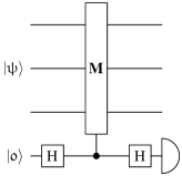
Figure 2.1: Quantum circuit for measuring the eigenvalue of a stabilizer operator.

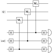
Figure 2.2: Quantum circuit for measuring the eigenvalue of a weight three stabilizer operator ${\bf M}={\bf M}_{1}\otimes{\bf M}_{2}\otimes{\bf M}_{3}$ fault-tolerantly. This generalizes in the obvious way for stabilizers of higher weight.

Because the data is made up of multiple qubits, and the stabilizer acts non-trivially over more than one of them, the circuit in Figure 2.1 is not fault-tolerant. This is because if one of the ${\tt CNOT}$s or ${\tt CSIGN}$s (for ${\bf X}$s and ${\bf Z}$s in ${\bf M}$ respectively, not shown in the figure) fails, it can cause an error on the control bit, which is shared by all the other controlled operations on other qubits. For example, if a failure occurs on the first controlled operation, all other qubits over which ${\bf M}$ acts non-trivially will be affected.

The solution for this problem is quite simple. If we replace the single control qubit by a group of qubits, one for each controlled operation needed to measure the stabilizer ${\bf M}$, and interact with the data transversally as depicted in Figure 2.2, there is no catastrophic error propagation. In this case, the control lines need to be replaced by a ’cat’ state, of the form

$$\left|{\mathfrak{0}}\right\rangle^{\otimes m}+\left|{\mathfrak{1}}\right\rangle^{\otimes m},$$ (2.30)

where $m$ is the number of qubits over which ${\bf M}$ acts non-trivially. If the error anticommutes with ${\bf M}$, this cat state will develop a relative phase of $-1$.

$$\left|{\mathfrak{0}}\right\rangle^{\otimes m}-\left|{\mathfrak{1}}\right\rangle^{\otimes m}.$$ (2.31)

Recall, however, equation (2.17), and take $C$ to be the $m$ bit repetition code – that is, a code that maps

$$0 \to \underbrace{00\cdots 0}_{\text{m times}}$$ (2.32a)

$$1 \to \underbrace{11\cdots 1}_{\text{m times}}.$$ (2.32b)

If we apply the qubitwise Hadamard to (2.31), we obtain a superposition of odd weight binary strings, and by measuring and computing the parity classically, we can fault-tolerantly detect that an error has occurred.

The use of cat states is necessary because it ensures that no information about the state of valid data is transfered to the ancilla. This is important because by measuring the ancilla we do not want to collapse the superposition of valid encoded states with no errors.

2.7 Threshold Theorem

Once the data is protected by an erasure correction code, the probability of erasure on the encoded data may still be unacceptably high. One way to get around this problem is to perform concatenated coding, that is, encode the encoded data once again. Say, for example, we have a code $C^{(1)}$ with parameters $[[n,1,d]]$. By concatenating the code with itself once, we obtain a $[[n^{2},1,d^{2}]]$ code which we call $C^{(2)}$, on which erasure correction can be seen as erasure correction on each level of concatenation separately. It is straightforward to see why the minimum distance scales in such a way. If $C$ has as its encoded operators $\overline{{\bf X}}$ and $\overline{{\bf Z}}$, then by replacing the uncoded Pauli operators by these encoded ones in the stabilizer of $C$, we obtain a new code $C^{(2)}$, which also includes the $n$-fold Cartesian product of the stabilizer of $C$. This procedure can be repeated $L$ times to obtain the concatenated code $C^{(L)}$ with parameters $[[n^{L},1,d^{L}]]$.

Consider $C^{(1)}$ once again. If the qubit erasure rate is $\epsilon$, then we can write the block failure rate as

$$\epsilon^{(1)}=\sum_{i=d}^{N}c_{i}\epsilon^{i},$$ (2.33)

where $c_{i}$ are integer coefficients dependent only on the erasure correction procedure and $i$. We are only interested in the case $d>2$, since we want to be able to correct at least one erasure. This recursion relation can be calculated by analyzing how erasures are introduced during the erasure correction procedure, and how this may lead to an uncorrectable erasure pattern in a code block, what we call a failure. In theory, one often assumes that erasure correction is attempted until the data is erasure free, leading $N$ to be infinite. In practice, however, only a certain maximal number of erasure correction steps are attempted, placing a bound on $N$.

Taking only the first term of the recursion relation (2.33), we can approximate the concatenated block failure rate as

$$\epsilon^{(L)}\approx c_{d}^{L}\epsilon^{d^{L}}.$$ (2.34)

In the case that $\epsilon^{(1)}<\epsilon$, then (2.34) indicates that the error rate of a concatenated code will drop doubly exponentially with $L$, while the size of the code block grown exponentially. This is, in essence, what is called the threshold theorem [1, 19, 23], which holds under various different conditions, but for our purposes it suffices to say that there is an limitless supply of fresh qubits, that the base erasure rate is independent of the size of the circuit, and that the probability of erasures on the different gates are independent. The value of $\epsilon$ which gives $\lim_{L\to\infty}\epsilon^{(L)}=0$ is called the erasure threshold, and obtaining such a value is the main focus of this thesis. In practice, this can be taken as the value of $\epsilon$ which gives $\epsilon^{(1)}<\epsilon$, as long as we assume that gate failures are independent, that the gate failure rate does not depend on the computation size, and that fresh qubits can be produced on demand. A much more detailed description of how to obtain the recursion relation (2.33) and how to extract the threshold will be given in Chapter 5.

Chapter 3 Efficient Linear Optics Quantum Computation

A very brief overview of the efficient linear optics quantum computing proposal by Knill, Laflamme and Milburn [18] is given, focusing on the behavior instead of implementation details. From that description, an error model is derived.

3.1 The Knill-Laflamme-Milburn proposal

One of the earliest proposals for a quantum computer, put forth by Chuang and Yamamoto [4], described a system where qubits were encoded in two photon modes – the so called dual rail encoding. In order to differentiate quantum states representing photon number states and quantum states representing the qubit, we follow the convention of using the standard font for number states, and the gothic font for qubits, so that the dual rail encoding of the $i$th qubit would be represented by

$$\left|{\mathfrak{0}}\right\rangle_{i} = \left|{0}\right\rangle_{a_{i}}\left|{1}\right\rangle_{b_{i}}$$ (3.1a)

$$\left|{\mathfrak{1}}\right\rangle_{i} = \left|{1}\right\rangle_{a_{i}}\left|{0}\right\rangle_{b_{i}},$$ (3.1b)

where $a_{i}$ and $b_{i}$ are the modes corresponding to qubit $i$. The main motivation of using photons to encode qubits is that photons do not decohere as easily as most other physical systems used to implement qubits, simply because photons can easily be made to not interact strongly with the environment.

One can use very simple optical elements to perform single qubit operations, and this was constructively proven well before the Chuang-Yamamoto proposal [24]. The elements used are called passive linear optics elements, and they are comprised of beam splitters (partially reflective mirrors) and phase shifters (delays). These elements have the property that they preserve the number of photons, and their behavior can easily be described by how they transform the photon creation operators of the modes involved.

However, it is very hard to make a universal set of quantum gates. In any universal set there is at least one entangling gate that requires the interaction of different qubits, and if the qubits are encoded as photons, it is very hard to construct such gates without using non-linear media to mediate the interaction. In [4], a Kerr non-linear medium was proposed to construct entangling gates, but Kerr media are notorious for having very high loss. Even measurements that require an implicit interaction of the qubits, such as Bell-basis measurements, are impossible to perform without failure [21]. It was thought that these facts comprised an informal “no-go” theorem for linear optics quantum computing, and various proposals that attempted to build quantum computers out of linear optics were shown to require an exponential amount of physical resources.

When Gottesman and Chuang [11] demonstrated that fault-tolerant universal quantum computation could be performed by using quantum teleportation and state preparation, this picture changed. The state preparation required for this gate construction scheme depends only on the gate being implemented, not on the inputs to the gate, so that if there is a way to prepare these states offline, linear optics quantum computation can indeed be performed (a fact that was pointed out in [11]). One just needs to keep trying to prepare this states until the preparation succeeds, or maintain many copies of the successfully prepared states.

Building on these ideas, Knill, Laflamme and Milburn put forth what is now commonly referred to as the KLM proposal for efficient linear optics quantum computation [18]. This proposal uses single photon sources and detectors, linear optics, and post-selection based on measurement outcomes.

There are two crucial parts of this proposal: the state preparation, and efficient teleportation. It was shown that one can build a non-deterministic non-linear sign change operation on a single photon mode, with knowledge of success or failure, using only linear optics and measurements. This gate, called ${\tt NS}_{-1}$, in effect performs the transformation

$$\left|{0}\right\rangle+\left|{1}\right\rangle+\left|{2}\right\rangle\to\left|{0}\right\rangle+\left|{1}\right\rangle-\left|{2}\right\rangle,$$ (3.2)

with a finite probability of success, which is detected by measuring some ancillary modes in the gate construction. Loose bounds have been placed on the success probability of constructions of this gate using only linear optics [15], and it is known that these gates cannot succeed with a probability of $\frac{1}{2}$ or more. One can construct a controlled phase flip, also known as a controlled sign or ${\tt CSIGN}$, using applications of the ${\tt NS}_{-1}$ and linear optics elements on the dual rail encoding. Direct computation with these gates is not scalable, but using the teleportation scheme proposed by [11], scalability is achieved by using these gates only in state preparation, where numerous attempts can be made until the gate performs the desired operation.

There is still the problem of how teleportation is performed. In the standard teleportation protocol, one needs entangled qubit pairs, which can be prepared offline, as well as Bell measurements. We have mentioned already that [21] showed that such measurements are impossible to perform without probabilistic failure – in fact, one cannot distinguish between two of the states in the four state Bell basis, and because of that, the probability of failure cannot be made less than $50\%$ if the input states are chosen uniformly over the Hilbert space. The alternative proposed in [18] is to use a modified protocol that relies on the preparation of a larger ancillary entangled state, the application of a Fourier transform involving the data to be teleported and the prepared state, and measurement of the ancillary states – the Fourier transform can be implemented efficiently using only linear optics. Given an ancillary state consisting of $N$ qubits, this teleportation protocol succeeds with probability $\frac{N}{N+1}$, a great improvement over the standard teleportation protocol. Note that $N=1$ is the base case with $\frac{1}{2}$ probability of success. This means one qubit is used for the teleportation, which seems to disagree with the knowledge that a Bell state is necessary for teleportation. However, only two of the four modes needed for the two qubit ${\tt CSIGN}$ operation interact with the ${\tt NS}_{-1}$ gates, so those are the only modes that need to be teleported, and each one requires two modes in a Bell state, resulting in one qubit per mode teleported.

3.2 The Error Model

Errors are introduced into computation in efficient linear optics quantum computation through various sources: failure of ${\tt CSIGN}$, photon loss, and finite accuracy of phase-shifters and beam-splitters, etc. Here we consider only failures during the application of a ${\tt CSIGN}$ that can be detected by measurement of the ancillary modes. In effect, this is not a detection of the failures of the ${\tt NS}_{-1}$ gates, but instead a detection of failures that occur during the teleportation of the qubits that realizes the ${\tt CSIGN}$ given the appropriate ancillary state. The ${\tt NS}_{-1}$ gates are used only in the state preparation for the teleportation, so we can choose to simply not use states resulting from failures of these gates.

Two failure modes are discussed here: teleportation failures that are inherent in the protocol because of limitations in linear optics, and failures due to photon loss at the detectors during teleportation.

3.2.1 Error model for ideal hardware

Assuming that all linear optics elements, all detectors and all sources are perfect, failures are still possible in the KLM proposal. This is due to the fact that teleportation succeeds with a probability less than unity, although these failures are always detected.

Consider how the ${\tt CSIGN}$ is teleported, abstracting from the details of linear optics, as depicted in Figure 3.1. The basic idea is to consider the teleportation of two qubits, followed by the application of a ${\tt CSIGN}$ between them. The commutation relations of ${\tt CSIGN}$ and the gates used for teleportation are used to rewrite the circuit in such a way that the ${\tt CSIGN}$ is applied between the prepared states used for the teleportation – see Section 2.4.2.

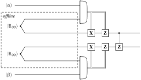
(a) Teleportation followed by a ${\tt CSIGN}$.

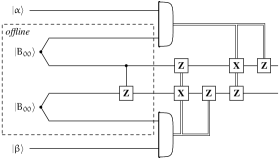
(b) ${\tt CSIGN}$ commuted backward into the prepared state, which is equivalent to (a).

Figure 3.1: The teleportation of a ${\tt CSIGN}$ gate [11, 18]. The states $\left|{B_{00}}\right\rangle$ are, in the simplest case, the Bell pair $\frac{1}{\sqrt{2}}\left(\left|{\mathfrak{00}}\right\rangle+\left|{\mathfrak{11}}\right\rangle\right)$. The two qubit measurement is performed over the Bell basis. Different Pauli corrections are applied to the output bit depending on the measurement outcomes, and this is indicated by the wider lines connected to the Pauli gates.

In general, the corrections dependent on the measurement outcomes must be applied to both qubits being teleported. However, it has been shown that the state preparation can be modified so that, if the teleportation of either qubit fails, it affects only that qubit. The protocol can be further engineered in a manner such that the failure can be taken to have occurred after the teleportation [18]. The effect of this type of failure, which is always detected, is that of a ${\bf Z}$ measurement of the qubit that is being teleported, with the measurement outcome made evident through the measurement part of the teleportation protocol. This occurs with probability $\frac{1}{N+1}$, where $N$ is the size of the ancilla state, which in the case of $N=2$ is simply the Bell state $\frac{1}{\sqrt{2}}\left(\left|{\mathfrak{00}}\right\rangle+\left|{\mathfrak{11}}\right\rangle\right)$.

One could, in principle, simply ignore the measurement outcome and take the teleportation failure to be a ${\bf Z}$ erasure, because the distinction between the two is classical information and classical processing, which we take to be perfect. Formally, this can be shown by the following proposition.

Proposition 1.

A projective ${\bf Z}$ measurement of unknown outcome at a known location is equivalent to a phase erasure.

Proof.

Expand the probabilistic application of the two possible projection operators for the eigenvectors of ${\bf Z}$

$${\bf Z}_{+} = \frac{1}{2}({\bf I}+{\bf Z})$$ (3.3a)

$${\bf Z}_{-} = \frac{1}{2}({\bf I}-{\bf Z}),$$ (3.3b)

onto a density matrix $\rho$. The probability of the outcome being the $+1$ eigenstate of ${\bf Z}$ is denoted by $\Pr({\bf Z}_{+})$, and for the $-1$ eigenstate is $\Pr({\bf Z}_{-})$, and since ${\bf Z}_{+}+{\bf Z}_{-}={\bf I}$, $\Pr({\bf Z}_{+})+\Pr({\bf Z}_{-})=1$. Ignoring the outcome of the measurement, $\rho$ will be transformed into $\mathbb{Z}(\rho)$ described by

$$\mathbb{Z}(\rho)= {\bf Z}_{+}\rho{\bf Z}_{+}+{\bf Z}_{-}\rho{\bf Z}_{-}$$ (3.4a)

$$= \frac{1}{4}({\bf I}+{\bf Z})\rho({\bf I}+{\bf Z})+\frac{1}{4}({\bf I}-{\bf Z})\rho({\bf I}-{\bf Z})$$ (3.4b)

$$= \frac{1}{2}\left(\rho+{\bf Z}\rho{\bf Z}\right),$$ (3.4c)

which is a ${\bf Z}$ erasure, as claimed. ∎

In this case, one would need to take the approach outlined in Section 2.6.1, and in the case of a CSS code, one would need to measure an ${\bf X}$ stabilizer in order to determine the syndrome of this erasure. This requires the application of ${\tt CNOT}$s, and since they are constructed from ${\tt CSIGN}$s conjugated by Hadamards (see Section 2.4.2), it is clear that the type of erasure introduced would be an ${\bf X}$ erasure, not a ${\bf Z}$ erasure. This is of particular importance for codes that can only correct ${\bf Z}$ erasures, like the codes used to obtain the $0.5$ threshold [14, 17], because it would lead to an immediate uncorrectable failure. In our case it desirable to avoid introducing different types of erasures, in order to simplify the analysis in Chapter 5.

In order not to introduce another type of erasure unnecessarily, we cannot use the standard fault-tolerant stabilizer measurement from the previous chapter. Instead, we extend a technique used for correcting ${\bf Z}$ measurements, which is described in detail in the next chapter.

For the purposes of describing the error model during computation, it suffices to say that each ${\tt CSIGN}$ has a probability $\epsilon_{i}$ of performing an unintentional ${\bf Z}$ measurement at either the control or the target qubit, independently. For simulation purposes, we can model this as a ${\bf Z}$ erasure at either target or control qubits independently, since from a ${\bf Z}$ erasure, with perfect detectors, one can easily obtain the measurement value without incurring any cost. Thus, with the first qubit being the control and the second being the target, the error model will be taken as

control failure $$: \mathbb{Z}\otimes{\bf I}$$ (3.5a)

target failure $$: {\bf I}\otimes\mathbb{Z},$$ (3.5b)

were the failures are taken to occur independently with probability $\epsilon_{i}$. Details of how the measurement outcome can be used to aid the correction step will be given in Section 4.1.3.

3.2.2 Error model for lossy detectors

Still assuming infinite precision in the parameters of the phase-shifters and beam-splitters, we can consider the possibility of photon loss due to detector inefficiencies. The dual-rail encoding of qubits ensures that as long as a qubit is properly encoded, there is in total a single photon between the two modes corresponding to the qubit, and since linear optics preserves the total photon number, measurement of ancillae allows for the detection of leakage from the dual-rail encoding.

In the original proposal for efficient linear optics quantum computation, a robust teleportation protocol called ${\bf RT}_{1}$ is described. This protocol has the property that it is able to detect the usual teleportation failures as well as photon losses both in the qubits used for teleportation (ancilla or data) as well as in the detectors. Like any possible linear optics implementation of teleportation, this teleportation circuit has only a finite probability of success even in the ideal case, and the ancilla measurement outcomes will indicate this type of failure that is not a consequence of photon loss. In the case of photon loss, however, the measurement outcomes will be different from the case of ideal failure, and as a side effect the modes of the qubit at the output of the teleportation are replaced with a fresh dual-rail encoded qubit in a fixed state [18]. This replacement by a fresh qubit corresponds to a total loss of information about the state of the qubit over which teleportation failed. We know that in the case of failure without photon loss we can model the output by a phase erasure, as demonstrated previously, but in the case of failure due to photon loss, we have the ingredients of a full erasure: knowledge of where the failure occurred (through the outcome of the ancilla measurements), and complete loss of knowledge about the state of the qubit.

We have already seen that in the case of a phase erasure, the qubit teleportations realizing the ${\tt CSIGN}$ are affected independently – if the teleportation of the control qubit fails, it does not imply that the target qubit teleportation fail, and vice-versa. This is not the case for the full erasure type of failure. Consider the teleportation of two quantum states, and the subsequent application of a ${\tt CSIGN}$ as in Figure 3.1. Taking a worst case approach, photon loss in the control part of the teleported ${\tt CSIGN}$ (top half of the figure) induces a ${\bf Z}$ error at the bottom whenever there is an ${\bf X}$ error at the top as well (this includes ${\bf Y}$ errors, since it is a combination of ${\bf Z}$ and ${\bf X}$ errors). A similar effect is observed in a photon loss at target part of the teleported ${\tt CSIGN}$. Clearly there is a classical correlation between the types of errors at the top qubit and the types of error at the bottom qubit – however, photon loss occurs independently at the top and bottom part of the teleported ${\tt CSIGN}$. Assuming perfect and instantaneous classical processing and communication, we could exploit this correlation in order to reduce the number of syndrome measurements that need to be performed. Ideally, because ${\tt CSIGN}$s are only applied transversely between different encoded blocks, one should choose to perform syndrome measurements on the block with fewer erasures, since one is less likely to induce a failure that way. In our worst case approximation, however, we ignore this classical correlation between the two encoded blocks of data, and we will restrict ourselves to the partial description of the two qubit output. Thus, taking the combined output to the ${\tt CSIGN}$ to be $\rho$, and the control and target states to be the result of a partial trace over $\rho$, that is $\rho_{\text{control}}=tr_{\text{target}}\rho$ and $\rho_{\text{target}}=tr_{\text{control}}\rho$, our error model can be seen as each type of failure inducing independent superoperators on the qubits as follows

control failure $$: \left\{\begin{array}[]{r@{\to}l}\rho_{\text{control}}&\mathbb{E}(\rho_{\text{control}})\\ \rho_{\text{target}}&\mathbb{Z}(\rho_{\text{target}}).\end{array}\right.$$ (3.6c)

target failure $$: \left\{\begin{array}[]{r@{\to}l}\rho_{\text{control}}&\mathbb{Z}(\rho_{\text{control}})\\ \rho_{\text{target}}&\mathbb{E}(\rho_{\text{target}}).\end{array}\right.$$ (3.6f)

Again, we assume that the probability that a photon loss failure has occurred in either teleportation is independent of the probability that a failure has occurred in the other teleportation. Moreover, we assume that only failures due to photon loss occur in this model, and we assume the probability of photon loss in a teleportation is given by $\epsilon_{l}$ under this model.

3.2.3 A mixed model

In general, depending on the gate construction, the probabilities of ideal teleportation failure and photon loss determines the error operator for failure of the qubit. However, in order to place a bound on the accuracy threshold for any gate construction, we consider only the end cases, $\Pr(\text{ideal failure}|\text{failure})=1$ and $\Pr(\text{photon loss failure}|\text{failure})=1$, which are the cases described above. It is important to emphasize that the two error models are very different – in one case we have ${\bf Z}$ measurements with known outcomes occuring independently at either qubit of the ${\tt CSIGN}$, while in the other we have, under our worst case approximation, both full and ${\bf Z}$ erasure occuring at either qubits of the ${\tt CSIGN}$. The actual error model will be a probabilistic mixture of the two models considered here.

We can restrict ourselves to considering only the end cases because, as will be demonstrated in later sections, the erasures that follow from photon loss have a higher cost than the ${\bf Z}$ measurements of the ideal model (i.e. more teleported gates need to be applied), so the threshold for any mixed error model will fall between the thresholds of these two end cases. This also provides further motivation for using essentially the same correction procedure to correct both ${\bf Z}$ measurements and ${\bf Z}$ erasures, since it simplifies and reduces the circuitry significantly.

Chapter 4 Candidate Codes

In this chapter a comparison is drawn between two small CSS codes, one being the Steane code, a $[[7,1,3]]$ code often used in threshold calculations for general errors, and the Grassl code, a $[[4,2,2]]$ code that is the smallest single erasure correcting code. Brief descriptions of universal sets of gates, as well as details of the erasure correction procedure, are given in order to justify the preference for the Steane code.

4.1 Steane Code

The Steane code [3, 27] was one of the first CSS codes to be discovered. Is it based on the $[7,4,3]$ classical Hamming code and its dual, the $[7,3,4]$ Simplex code, yielding a $[[7,1,3]]$ quantum code that allows for very simple fault-tolerant computation. The 7-bit Hamming code has parity check matrix

$$H_{[7,4,3]}=\left[\begin{array}[]{ccccccc}1&1&1&1&0&0&0\\ 1&1&0&0&1&1&0\\ 1&0&1&0&1&0&1\end{array}\right],$$ (4.1)

so following the CSS construction of self-orthogonal classical codes in Section 2.4.1, we find that the stabilizer $S$ is generated by

$$\begin{array}[]{ccccccccccccccl}{\bf M_{1}}&=&{\bf X}&\otimes&{\bf X}&\otimes&{\bf X}&\otimes&{\bf X}&\otimes&{\bf I}&\otimes&{\bf I}&\otimes&{\bf I}\\ {\bf M_{2}}&=&{\bf X}&\otimes&{\bf X}&\otimes&{\bf I}&\otimes&{\bf I}&\otimes&{\bf X}&\otimes&{\bf X}&\otimes&{\bf I}\\ {\bf M_{3}}&=&{\bf X}&\otimes&{\bf I}&\otimes&{\bf X}&\otimes&{\bf I}&\otimes&{\bf X}&\otimes&{\bf I}&\otimes&{\bf X}\\ {\bf M_{4}}&=&{\bf Z}&\otimes&{\bf Z}&\otimes&{\bf Z}&\otimes&{\bf Z}&\otimes&{\bf I}&\otimes&{\bf I}&\otimes&{\bf I}\\ {\bf M_{5}}&=&{\bf Z}&\otimes&{\bf Z}&\otimes&{\bf I}&\otimes&{\bf I}&\otimes&{\bf Z}&\otimes&{\bf Z}&\otimes&{\bf I}\\ {\bf M_{6}}&=&{\bf Z}&\otimes&{\bf I}&\otimes&{\bf Z}&\otimes&{\bf I}&\otimes&{\bf Z}&\otimes&{\bf I}&\otimes&{\bf Z},\end{array}$$ (4.2)

Because the structure of the stabilizer generators is directly derived from the parity check matrix, it immediately follows that the derived CSS code has the same minimum distance as the classical Hamming code, as argued in Section 2.4.1.

4.1.1 Fault-tolerant Universal Gates

Being a self-orthogonal CSS code, the Steane code has a very simple fault-tolerant implementation of encoded gates. Shor [26] was the first to demonstrate how universal fault-tolerant computation could be performed on the Steane code by explicitly constructing a fault-tolerant encoded Toffoli using only measurements and encoded Clifford gate operations. We follow his approach by first giving the encoded Clifford gates demonstrated by Gottesman [10], and then use insights by Zhou et al. [33] to demonstrate how a generating set for the Clifford group ${\mathscr{C}}_{2}$ can be constructed.

First, we need to implement the Pauli operators. Following the stabilizer formalism, we can choose members of the normalizer $N(S)$ of the stabilizer that obey the commutation relations for the Pauli operators, namely:

$$\{\overline{{\bf X}},\overline{{\bf Z}}\}=0$$ (4.3a)

$$\overline{{\bf X}}\overline{{\bf Z}}=\overline{{\bf Y}}.$$ (4.3b)

This choice of encoded Pauli operators is equivalent to choosing the encoded basis states, and it is equally non-unique. One such choice is:

$$\overline{{\bf X}} = {\bf I}\otimes{\bf I}\otimes{\bf I}\otimes{\bf I}\otimes{\bf X}\otimes{\bf X}\otimes{\bf X}$$ (4.4a)

$$\overline{{\bf Z}} = {\bf I}\otimes{\bf I}\otimes{\bf I}\otimes{\bf I}\otimes{\bf Z}\otimes{\bf Z}\otimes{\bf Z},$$ (4.4b)

but one could just as well call the first operator $\overline{{\bf Z}}$ and the second one $\overline{{\bf X}}$, and the computational basis would be changed to whatever the eigenbasis of $\overline{{\bf Z}}$ is. These operations do not require interaction between different qubits so they are automatically fault-tolerant, and this is always the case for encoded Pauli operations based on the normalizer of the stabilizer code.

The next step is to show the construction of the encoded Clifford gates not in ${\mathcal{P}}_{k}$. We have seen that the Hadamard gate maps between ${\bf X}$ and ${\bf Z}$ and leaves the other Pauli operators invariant, and, by construction of the Steane code, every stabilizer operator that is made up of only ${\bf X}$s has a counterpart that is made up of only ${\bf Z}$s, so applying the the Hadamard transversally preserves the stabilizer, and therefore it preserves the codespace. Given our choice of $\overline{{\bf X}}$ and $\overline{{\bf Z}}$, it is also clear that this operation is the encoded Hadamard itself. The phase gate ${\bf P}$ can similarly be applied qubitwise to map the all ${\bf X}$s stabilizer generators into all ${\bf Y}$s operators with an added phase factor, but this is only a valid encoded operation if these operators made up of only ${\bf Y}$s are in the stabilizer. Given that

$${\bf P}{\bf X}{\bf P}^{\dagger} = i{\bf Y}$$ (4.5a)

$${\bf P}{\bf Z}{\bf P}^{\dagger} = {\bf Z},$$ (4.5b)

we would like the weight of the all ${\bf X}$s and all ${\bf Z}$s stabilizer generators be a multiple of four so that the $\frac{\pi}{2}$ complex phases add up to a $0$ phase. Fortunately, the Steane code is a doubly-even CSS code, so all stabilizer generators have weight four. The operation that this qubitwise ${\bf P}$ performs on the encoded operators is

$${\bf P}^{\otimes 7}\overline{{\bf X}}\left({\bf P}^{\dagger}\right)^{\otimes 7} = {\bf I}\otimes{\bf I}\otimes{\bf I}\otimes{\bf I}\otimes i{\bf Y}\otimes i{\bf Y}\otimes i{\bf Y}$$ (4.6a)

$$= -i{\bf I}\otimes{\bf I}\otimes{\bf I}\otimes{\bf I}\otimes{\bf Y}\otimes{\bf Y}\otimes{\bf Y}$$ (4.6b)

$$= -i\overline{{\bf Y}}=-i\overline{{\bf X}{\bf Z}}$$ (4.6c)

$$= \overline{{\bf P}}^{\dagger}\overline{{\bf X}}\overline{{\bf P}},$$ (4.6d)

The qubitwise phase gate realizes the encoded inverse phase gate. In order to get the encoded phase gate itself, one only needs to apply the inverse phase gate qubitwise.

These constructions of the single qubit Clifford group operations for the Steane code are much more robust and desirable than the constructions for the same gates for the Grassl code derivatives, as will be shown later. The main reason for this robustness is the fact that no two qubit interactions were necessary for any of these constructions, only single qubit operations. In the context of the KLM proposal for linear optics quantum computing, this is a powerful advantage, because it allows us to take these operations to be erasure free in the ideal model, and loss free in our simple lossy model.

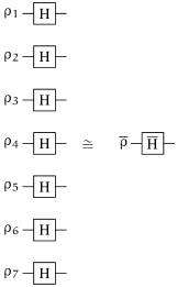
(a) Hadamard Gate

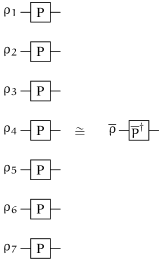
(b) phase gate

Figure 4.1: Transversal one qubit Clifford gates for the Steane code.

All we need to complete the generating gates of ${\mathscr{C}}_{2}$ is the encoded ${\tt CNOT}$. For the construction of the encoded ${\tt CNOT}$ itself, it is unavoidable that two qubit interactions be present. All CSS codes allow for transversal ${\tt CNOT}$ application as an encoded operation, and in all these cases the encoded operation that is applied is itself the encoded ${\tt CNOT}$ [10]. This follows again from the fact that the stabilizer generators are made up of either ${\bf X}$s or ${\bf Z}$s but not both, and following how the ${\tt CNOT}$ maps between Pauli operators, it becomes clear that the mapping will preserve $S\times S$. A quick calculation demonstrates that

$$\overline{{\bf X}}\otimes{\bf I} \to \overline{{\bf X}}\otimes\overline{{\bf X}}$$ (4.7a)

$$\overline{{\bf Z}}\otimes{\bf I} \to \overline{{\bf Z}}\otimes{\bf I}$$ (4.7b)

$${\bf I}\otimes\overline{{\bf X}} \to {\bf I}\otimes\overline{{\bf X}}$$ (4.7c)

$${\bf I}\otimes\overline{{\bf Z}} \to \overline{{\bf Z}}\otimes\overline{{\bf Z}},$$ (4.7d)

as claimed.

Figure 4.2: Encoded ${\tt CNOT}$ for the Steane code.

The Clifford group is not sufficient for universal quantum computation. However, almost any additional gate that lies outside ${\mathscr{C}}_{2}$ gives us a universal set, and the gates that are usually considered are the Toffoli gate or the $\frac{\pi}{8}$ gate, which are known to give a universal set when combined with the Clifford group. The first fault-tolerant construction of the Toffoli for the Steane code was given by Shor [26], and a fault-tolerant construction of the $\frac{\pi}{8}$ gate was given by Boykin et al. [22]. Neither of these constructions was seen to follow the same general framework, but Zhou et al. [33] demonstrated how they follow directly from an extension of the work by Gottesman and Chuang [11] on universal quantum computation using teleportation and single qubit operations.

The detailed analysis of how these constructions were obtained will not be given here, but for illustration the resulting circuits implementing the $\frac{\pi}{8}$ gate and the Toffoli gate are given in Figure 4.3. Zhou et al. show how to prepare the state in the dotted box fault-tolerantly . The construction of the Toffoli involves not only the three required ${\tt CNOT}$s used to perform a simplified teleportation protocol, but also classically controlled application of ${\tt CNOT}$s and ${\tt CSIGN}$s depending on the measurement outcomes. This Toffoli construction still has a threshold very close to the Clifford gate threshold when the state preparation yield similar failure probabilities as the Clifford gate failure probabilities [8].

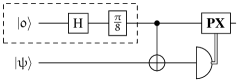
(a) $\frac{\pi}{8}$ gate

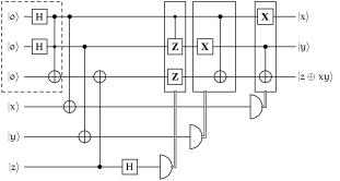
(b) Toffoli gate

Figure 4.3: Fault-tolerant gates needed for universal computation, as depicted in [33]. All measurements are in the ${\bf Z}$ eigenbasis. The dashed boxes represent states that can be prepared off-line fault-tolerantly, the double lines represent classical control dependent on the measurement outcome.

Given our error model, where ${\tt CNOT}$s/${\tt CSIGN}$s are costly compared to single qubit gates, it can be intuitively seen that the encoded $\frac{\pi}{8}$ gate should give a threshold much closer to the Clifford gate threshold under the same conditions because it requires fewer applications of such gates. This will be the operating assumption for the rest of the analysis, and from now on we focus only on the threshold for Clifford gates.

4.1.2 Erasure Correction

The Steane code is a $[[7,1,3]]$ quantum code, so immediately it is clear that it will be able to correct all weight two and one erasure patterns. This can be done by measuring the generators of the stabilizer of the code and inferring the erasure operators from the commutation properties measured – the collection of all measurements is known as the syndrome of the error.

One can check explicitly which erasure patterns are correctable by applying the modified Knill-Laflamme condition to all possible erasure operators for a given erasure pattern. Taking the approach of checking the correctability of ${\bf X}$ erasure and ${\bf Z}$ erasures separately simplifies the analysis somewhat – we can say that a pattern is correctable if the ${\bf X}$ erasure patterns and the ${\bf Z}$ erasure pattern are correctable. Through this brute force approach, one finds that only $28$ of the possible ${7\choose 3}=35$ weight three patterns, $\frac{4}{5}$ of the total, are correctable.

All stabilizer generators have weight four, so any stabilizer measurement can lead at most to failures in four qubits. If we would like to measure the syndrome of a single erasure, we simply choose stabilizers which act non-trivially over the qubit that has been erased. If there are two erasures, it turns out that one can always choose a stabilizer that will act non-trivially on either of the erasures but not on the other one [32]. If we consider single failures on any of the erasure free qubits being touched by the stabilizer measurement, we find that $\frac{2}{3}$ of all reachable weight three erasure patterns are correctable, but the other $\frac{1}{3}$ are uncorrectable. This is always the case, regardless of which of the two erasures we choose to correct, or which stabilizer we choose to measure (given the constraint that we do want to correct one erasure when we measure a stabilizer operator).

Depending on the type of erasure, a different number of stabilizer operators need to be measured. In particular, since a ${\bf Z}$ erasure just needs to be checked for commutation against an ${\bf X}$ stabilizer, and a ${\bf X}$ erasure just against a ${\bf Z}$ stabilizer, it follows that a full erasure needs two stabilizer measurements.

Exactly how the correctability of these erasure patterns can be easily determined, as well as which patterns are reachable after the erasure correcting procedure is applied to a given pattern, will be elucidated in Chapter 5.

4.1.3 Z Measurement Correction

As mentioned in the previous chapter, we would like to avoid using ${\tt CNOT}$s to measure the ${\bf X}$ stabilizer of a CSS code. An alternative method has been developed that allows for measurement of the syndrome and correction of the error to be done in a single step, as long as the outcome of the ${\bf Z}$ measurement is available [14, 17, 18].

In order to correct the ${\bf Z}$ measurement, we need to, indirectly, measure an ${\bf X}$ stabilizer that acts non-trivially over a single ${\bf Z}$ measurement. Since the Steane code only has weight four ${\bf X}$ stabilizers, we can consider only the four qubits over which the stabilizer acts non-trivially, so the stabilizer can be rewritten

$${\bf X}\otimes{\bf X}\otimes{\bf X}\otimes{\bf X},$$ (4.8)

with $+1$ eigenvalue eigenvectors

$$\frac{1}{\sqrt{2}}(\left|{\mathfrak{0000}}\right\rangle+\left|{\mathfrak{1111}}\right\rangle) = \left|{\gamma_{1}}\right\rangle$$ (4.9)

$$\frac{1}{\sqrt{2}}(\left|{\mathfrak{0101}}\right\rangle+\left|{\mathfrak{1010}}\right\rangle) = \left|{\gamma_{2}}\right\rangle$$ (4.10)

$$\frac{1}{\sqrt{2}}(\left|{\mathfrak{0011}}\right\rangle+\left|{\mathfrak{1100}}\right\rangle) = \left|{\gamma_{3}}\right\rangle$$ (4.11)

$$\frac{1}{\sqrt{2}}(\left|{\mathfrak{0110}}\right\rangle+\left|{\mathfrak{1001}}\right\rangle) = \left|{\gamma_{4}}\right\rangle.$$ (4.12)

Without loss of generality, take the first qubit to be the qubit that has undergone a ${\bf Z}$ measurement, and we apply an ${\bf X}$ on all remaining qubits if the outcome is $\left|{\mathfrak{1}}\right\rangle$, and do nothing otherwise. If initially we have some state

$$\sum_{i=1}^{4}\alpha_{i}\left|{\gamma_{i}}\right\rangle,$$ (4.13)

then after the measurement (and possible ${\bf X}$ applications) we will have the state

$$\left|{\mathfrak{p}}\right\rangle=\sum_{i=1}^{4}\alpha_{i}\left|{\tilde{\gamma}_{i}}\right\rangle,$$ (4.14)

where, if we consider only the non-measured qubits, we have

$$\left|{\tilde{\gamma}_{1}}\right\rangle = \left|{\mathfrak{000}}\right\rangle$$ (4.15)

$$\left|{\tilde{\gamma}_{2}}\right\rangle = \left|{\mathfrak{101}}\right\rangle$$ (4.16)

$$\left|{\tilde{\gamma}_{3}}\right\rangle = \left|{\mathfrak{011}}\right\rangle$$ (4.17)

$$\left|{\tilde{\gamma}_{4}}\right\rangle = \left|{\mathfrak{110}}\right\rangle.$$ (4.18)

In order to obtain the original state back, we need a fresh qubit in the state $\left|{+}\right\rangle=\frac{1}{\sqrt{2}}\left(\left|{\mathfrak{0}}\right\rangle+\left|{\mathfrak{1}}\right\rangle\right)$, so we apply the circuit in Figure 4.5. Since this circuit is made up of only ${\mathscr{C}}_{2}$ gates, we can consider the teleportation of the state $\left|{\mathfrak{p}}\right\rangle$ before applying Figure 4.5, and then simply commute that part of the circuit into the state preparation part of the teleportation protocol – the only qubit introduced is in the fixed state $\left|{+}\right\rangle$, so it can be taken into the state preparation part as well.

It is important that we use the slightly modified teleportation protocol shown in Figure 4.4. In this qubit teleportation protocol, the only source of failure is the two qubit gate $({\bf Z}{\bf Y})_{90^{\circ}}$, which is performed through a ${\tt CSIGN}$ conjugated by one qubit ${\mathscr{C}}_{2}$ gates (the other two qubit gates are performed similarly). This teleportation protocol guarantees that if there is a failure in the $({\bf Z}{\bf Y})_{90^{\circ}}$ gate, it will translate to a ${\bf Z}$ measurement of the qubit being teleported. Because of the structure of the circuit in Figure 4.5, only the ${\bf Z}$ corrections of the teleportation will propagate through the ${\tt CNOT}$s, and therefore so will the ${\bf Z}$ measurements.

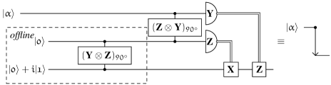
Figure 4.4: Modified teleportation protocol introducing only ${\bf Z}$ measurements in case of the failure of the $({\bf Z}\otimes{\bf Y})_{90^{\circ}}$ gate

Figure 4.5: Circuit taking the state $\left|{\mathfrak{p}}\right\rangle$ into an eigenvalue $+1$ eigenvector of ${\bf X}\otimes{\bf X}\otimes{\bf X}\otimes{\bf X}$.

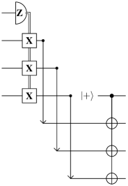
Figure 4.6: Full circuit for correction of a single ${\bf Z}$ measurement. The ${\tt CNOT}$s can be commuted backwards in time and combined with the offline state preparation for the teleportations.

If any of the teleportations fail, the corresponding qubit undergoes a ${\bf Z}$ measurement, but also the correction target, the qubit we were trying to recover, cannot be corrected. Taking each teleportation to fail with a probability $\epsilon_{i}$, the correction will succeed with probability $(1-\epsilon_{i})^{3}$, and if we take $\mathbb{Z}$ to signify the ${\bf Z}$ measurement, we have the following transition probabilities on the four qubits in question

$$\Pr({\bf I}\otimes{\bf I}\otimes{\bf I}\otimes{\bf I}|\mathbb{Z}\otimes{\bf I}\otimes{\bf I}\otimes{\bf I}) = (1-\epsilon_{i})^{3}$$ (4.19)

$$\Pr(\mathbb{Z}\otimes\mathbb{Z}\otimes{\bf I}\otimes{\bf I}|\mathbb{Z}\otimes{\bf I}\otimes{\bf I}\otimes{\bf I}) = \epsilon_{i}(1-\epsilon_{i})^{2}$$ (4.20)

$$\Pr(\mathbb{Z}\otimes\mathbb{Z}\otimes\mathbb{Z}\otimes{\bf I}|\mathbb{Z}\otimes{\bf I}\otimes{\bf I}\otimes{\bf I}) = \epsilon_{i}^{2}(1-\epsilon_{i})$$ (4.21)

$$\Pr(\mathbb{Z}\otimes\mathbb{Z}\otimes\mathbb{Z}\otimes\mathbb{Z}|\mathbb{Z}\otimes{\bf I}\otimes{\bf I}\otimes{\bf I}) = \epsilon_{i}^{3}$$ (4.22)

with the other patterns with equal weights being obtained by permutation, preserving the probabilities of transition.

In this analysis, we have neglected the remaining three qubits of the Steane code, and we have assumed that the state described by the four qubits in question was a pure state, which is not true. In reality, the state of those 4 qubits will be a mixture, because the seven qubits of the code block are entangled, but similar results in that case follow by linearity from the results given here.

With the method described here, we can correct ${\bf Z}$ measurements without directly measuring ${\bf X}$ stabilizers. We can employ the exact same method to correct ${\bf Z}$ erasures by first measuring the erased qubit in the ${\bf Z}$ basis, and then simply replacing it with a qubit corresponding to the measurement outcome. Once the measurement outcome is known, this same procedure can be used.

In the case of a qubit loss in any of the three teleportations, we take the worst case approach once more. Thus, the qubit being teleported is completely erased, and the ${\bf Z}$ erased qubit that is being corrected is ${\bf Z}$ erased once more. Each of the three teleportations can lose a photon independently, so the transition probabilities can easily be computed for the lossy model as well, yielding

$$\Pr({\bf I}\otimes{\bf I}\otimes{\bf I}\otimes{\bf I}|\mathbb{Z}\otimes{\bf I}\otimes{\bf I}\otimes{\bf I}) = (1-\delta)(1-\epsilon_{l})^{3}$$ (4.23)

$$\Pr(\mathbb{E}\otimes{\bf I}\otimes{\bf I}\otimes{\bf I}|\mathbb{Z}\otimes{\bf I}\otimes{\bf I}\otimes{\bf I}) = \delta$$ (4.24)

$$\Pr({\bf Z}\otimes\mathbb{E}\otimes{\bf I}\otimes{\bf I}|\mathbb{Z}\otimes{\bf I}\otimes{\bf I}\otimes{\bf I}) = (1-\delta)\epsilon_{l}(1-\epsilon_{l})^{2}$$ (4.25)

$$\Pr({\bf Z}\otimes\mathbb{E}\otimes\mathbb{E}\otimes{\bf I}|\mathbb{Z}\otimes{\bf I}\otimes{\bf I}\otimes{\bf I}) = (1-\delta)\epsilon_{l}^{2}(1-\epsilon_{l})$$ (4.26)

$$\Pr({\bf Z}\otimes\mathbb{E}\otimes\mathbb{E}\otimes\mathbb{E}|\mathbb{Z}\otimes{\bf I}\otimes{\bf I}\otimes{\bf I}) = (1-\delta)\epsilon_{l}^{3},$$ (4.27)

with the factors involving $\delta$, the probability of a detector failing, arising due to the fact that we need to perform a ${\bf Z}$ measurement explicitly.

4.1.4 The Encoded Error Model

In the case of a failure in correction an error in a code block, it is important to understand what kind of error is induced in the encoded qubit. This encoded error model is crucial for predicting the performance when the information is encoded multiple times, an approach that will be used in the Chapter 5.

For the error models considered in Chapter 3, this is a relatively simple problem that can be solved with the help of the stabilizer and normalizer formalisms.

Error Model for Ideal Hardware

In this error model, all erasures are ${\bf Z}$ measurements, and from the structure of the Steane code, it is known which patterns of erasures are correctable and which ones are not. Consider the case of the ${\bf Z}$ measurement of the last 3 qubits of a code block, which is not correctable. Since the encoded ${\bf Z}$ operation consists of ${\bf Z}$s applied to the last 3 qubits, as described by (4.4b), it is clear that this uncorrectable error is equivalent to an encoded ${\bf Z}$ measurement on the encoded qubit. Consider, on the other hand, the case of ${\bf Z}$ measurements on all qubits of the code block. Since, given the stabilizer operator ${\bf M}_{4}$ from (4.2), $\overline{{\bf Z}}{\bf M}_{4}={\bf Z}\otimes{\bf Z}\otimes{\bf Z}\otimes{\bf Z}\otimes{\bf Z}\otimes{\bf Z}\otimes{\bf Z}$, it is clear that this is also equivalent to a $\overline{{\bf Z}}$ measurement. It turns out that because of this, all uncorrectable weight three measurement patterns (as well as the weight seven pattern) are equivalent to a $\overline{{\bf Z}}$ measurement. All uncorrectable measurement patterns of intermediate weight can be thought of as a uncorrectable weight three measurement pattern followed by some additional measurements, so that all of them are equivalent to a $\overline{{\bf Z}}$ measurement.

In practice, it is also important to consider the cases of correctable erasure patterns, since a code block may end up in such a state after some finite number of error correcting rounds. This is extremely simple for the case of ideal hardware, since we can simply measure any number of qubits perfectly, allowing us to force an uncorrectable measurement pattern, which as shown above is always a $\overline{{\bf Z}}$ measurement.

Thus, the encoded error model is identical to the base error model up to different probability distributions.

Error Model for Lossy Detectors

Given the correspondence between ${\bf Z}$ erasures and ${\bf Z}$ measurements of unknown outcome, failures consisting only of ${\bf Z}$ erasures have a behavior that parallels failures consisting only of ${\bf Z}$ measurements.

The stabilizer generators for the Steane code that are tensor products of ${\bf X}$s only have exactly the same structure as the stabilizer generators that are tensor products of ${\bf Z}$s only, and a full erasure is the composition of a ${\bf Z}$ erasure and an ${\bf X}$ erasure, so uncorrectable erasure patterns consisting only of full erasures are equivalent to encoded full erasures.

Uncorrectable erasure patterns that include both ${\bf Z}$ and full erasures need to be considered as composition of ${\bf Z}$ and ${\bf X}$ erasures patterns. With the error correction scheme described in the previous sections of this chapter, we can only have ${\bf X}$ erasures on qubits that have ${\bf Z}$ erasures as well – that is to say that we only have ${\bf Z}$ or full erasures, but no ${\bf X}$ erasures. If the ${\bf X}$ erasure pattern is uncorrectable, then the encoded failure will be an encoded full erasure, since we are guaranteed to also have an uncorrectable ${\bf Z}$ erasure pattern. On the other hand, if the ${\bf X}$ erasure pattern is correctable, we can simply attempt to correct ${\bf X}$ erasures until either there are no more full erasures (in which case we would only have the uncorrectable ${\bf Z}$ erasure pattern, which corresponding to an encoded ${\bf Z}$ erasure), or until the ${\bf X}$ erasure pattern is uncorrectable (in which case we would have the encoded full erasure).

Correctable erasure patterns are a little more complex since they require the measurement of all qubits in order to be interpreted as encoded errors, and because of the lossy nature of the detectors, the outcome could be either an encoded ${\bf Z}$ measurement, or an encoded full erasure. The probabilities of each of these outcomes depends on the probability of failure of the qubit measurements, so this extra measurement needs to be regarded as a separate step after the desired rounds of error correction. In the best case, where no measurements fail, we obtain an encoded ${\bf Z}$ measurement, while in the worst case, we obtain an encoded full erasure. As shown before, measuring all qubits in the ${\bf Z}$ eigenbasis is equivalent to an encoded ${\bf Z}$ measurement. Moreover, because of the structure of the Steane code, even though some of these measurements may fail, the encoded measurement outcome may still be inferred by applying classical error correction techniques to the outcomes. If recovery is not possible because of the high number of errors, then the failure is an encoded full erasure. We can take these correctable erasure patterns to be encoded ${\bf Z}$ erasures, since, like ${\bf Z}$ erasures, they require ${\bf Z}$ measurements to be performed as the first step of the error correction, and failure of the measurement yields a full erasure.

Once again, the encoded error model is identical to the base error model up to a different probability distribution.

A Mixed Error Model

In a mixed error model, where we have both the limitations of linear optics and the post-selection based construction of the ${\tt CSIGN}$ as well as the imperfect photon detectors, the error model changes only quantitatively. At higher levels of encoding we still expect to find ${\bf Z}$ measurements as well as ${\bf Z}$ and full erasures, but qualitative analysis shows that there is a bias towards the more benign error model.

A failure pattern than includes both ${\bf Z}$ erasures and ${\bf Z}$ measurements (but no full erasures) can be taken as an encoded ${\bf Z}$ erasure at no additional cost, or may be taken as an encoded ${\bf Z}$ measurement at the cost of measuring the ${\bf Z}$ erasures, possibly introducing full erasures which may lead to encoded full erasures. If the measurement can be inferred without measuring the ${\bf Z}$ erasures by using classical error correction, the probability of encoded full erasures is reduced. Failure patterns that include full erasures are treated similarly.

The procedure for turning correctable failures into failures at a higher level of encoding could either yield ${\bf Z}$ measurements, full erasures or ${\bf Z}$ erasures. In particular, there is no need to explicitly measure qubits that have been affected by an unintentional measurement, which also reduces the probability of encoded full erasures.

Both these opportunities for gain over the purely lossy error model indicate that the mixed error model should always allow for improvement over the purely lossy error model, and that it will be naturally biased towards the ideal detector error model.

Worst Case Analysis

For the calculations made in Chapters 5, we take all encoded errors in the error model for lossy detectors to be full erasures. This worst case approach simplifies the calculations significantly, and although it gives a looser lower bound to the error threshold, it will be shown to be enough to match predictions in [17, 18].

Formally one usually takes the threshold to be the break even point between the encoded and the base error rates. Here we will take the threshold to be the point where the encoded error rate is half of the base error rate. This is because the probability of full erasure of a qubit given a failure has occured is the same as the probability of a ${\bf Z}$ erasure given a failure has occured – that is, both occur with conditional probability $\frac{1}{2}$. Thus, since we take all encoded failures to be full erasures, we apply the break even condition to full erasures only, which translates to the requirement that the overall encoded failure rate be half of the base failure rate. When the threshold is explicitly calculated in Section 5.1, this relationship will be formalized more clearly.

4.2 Grassl Code

Grassl, Beth and Pellizzari [12] have shown that the shortest possible erasure code is a $[[4,2,2]]$ code, which is referred to here as the Grassl code. This is a CSS code derived from the classical code consisting of all even weight strings of length four. It corrects a single erasure, the general class of such distance two codes having been discussed in detail in [10]. The stabilizer group $S$ of this code is generated by the operators

$$\begin{array}[]{ccccccccc}{\bf M}_{1}&=&{\bf X}&\otimes&{\bf X}&\otimes&{\bf X}&\otimes&{\bf X}\\ {\bf M}_{2}&=&{\bf Z}&\otimes&{\bf Z}&\otimes&{\bf Z}&\otimes&{\bf Z},\end{array}$$ (4.28c)

and a generating set for the encoded Pauli operators is

$$\begin{array}[]{cccccccc}\overline{{\bf X}}_{1}=&{\bf X}&\otimes&{\bf X}&\otimes&{\bf I}&\otimes&{\bf I}\\ \overline{{\bf X}}_{2}=&{\bf X}&\otimes&{\bf I}&\otimes&{\bf I}&\otimes&{\bf X}\\ \overline{{\bf Z}}_{1}=&{\bf Z}&\otimes&{\bf I}&\otimes&{\bf I}&\otimes&{\bf Z}\\ \overline{{\bf Z}}_{2}=&{\bf Z}&\otimes&{\bf Z}&\otimes&{\bf I}&\otimes&{\bf I},\end{array}$$ (4.29e)

The fact that all operators in the generating set of the encoded Pauli operators are of weight two proves that this is a distance two code – that is, there are weight two error operators that will map valid codewords into different valid codewords, and will therefore be undetectable and uncorrectable.

4.2.1 Fault-tolerant Universal Gates

One difference between the Grassl code and the Steane code that is immediately obvious is the fact that the Grassl code encodes two qubits. This raises the question of how to concatenate the code, and how the different choices affect the performance. Even if this issue is resolved, because we have two encoded qubits, we must consider different types of encoded operations dealing with the different encoded qubits. While there are very simple constructions of some of these gates – such as an encoded ${\tt CNOT}$ between the two encoded qubits in a block or the ${\tt SWAP}$ between these same qubits – the construction of other types of ${\tt CNOT}$s have a very high cost because of the use of multiple rounds of teleportation and multiple ancilla preparations – some gates that suffer this problem are the encoded ${\tt CNOT}$ between the individual encoded qubits of two different blocks.

On the other hand, one may choose to bypass this problem by modifying the Grassl code to encode a single qubit. That can be done by choosing one of the encoded Pauli operators over a single encoded qubit and making it a stabilizer. Any such choice is valid since we know that all operators in $N(S)$ commute with the elements of $S$ (see Section 2.4.2), and that results in a stabilizer code with three stabilizer generators, as desired ($n-k=4-1$ since we want a $[[4,1]]$ code). It is easy to check that the minimum distance of the code remains the same, so we are able to correct a single erasure with this code. The main problem is that the resulting code is not a self-orthogonal CSS code, but a more general form of CSS code. While the encoded ${\tt CNOT}$ can easily be implemented by qubitwise ${\tt CNOT}$s, neither the encoded Hadamard nor the encoded Phase gates can be implemented as easily. Instead, it is necessary to use ancillary states, multiple ${\tt CNOT}$s and single qubit operations to generate these two remaining encoded Clifford gates [10]. This is highly undesirable for the error models under consideration because this translates to encoded single qubit operations that can introduce erasures, while in the Steane code those operations can never introduce erasures.

A similar problem is found even if the Grassl code is maintained in its original form. The encoded single qubit operations that are applied only to one encoded qubit, while the identity is applied to the other, require complex protocols involving teleportations and measurements. Thus, there is strong evidence that the Grassl code is suboptimal for fault-tolerant quantum computation in the error model given for linear optics quantum computation.

Chapter 5 The Erasure Threshold

A novel method for determining the recursion relation for the encoded failure rate is given. This method describes the erasure correction procedure as a random walk over equivalence classes of erasure patterns, allowing for a compact description that can give the recursion relation for any number of erasure correction attempts. Using this technique, the recursion relations for the Steane code under the ideal and lossy error models are given, and values for the threshold are estimated numerically.

5.1 Calculation of the Threshold

In order to calculate the error threshold, we need to calculate the recursion relation for the probability of error $\epsilon^{(L)}$ in encoding level $L$ in terms of the probability of error $\epsilon^{(L-1)}$ in encoding level $L-1$. For simplicity, we consider only the relationship between the first level of encoding and the base error rate, that is,

$$\epsilon^{(1)}=\sum_{n=m}^{\infty}c_{n}\epsilon^{n},$$ (5.1)

where $\epsilon$ is the error rate at the physical qubits, $c_{n}$ are constant integers dependent only on $n$, and $m$ is the minimum number of failures causing an unrecoverable error, as we have seen in Chapter 2.

In the general case one needs to keep track of the possible propagation of undetected errors, but the erasure error model allows us to ignore this complication because the presence and location of erasures is known by definition. Thus, we only apply the erasure correction procedure when we know an erasure has occurred, and any additional failure that occurs during erasure correction is immediately flagged, so we can keep applying the erasure correction procedure until the data is erasure free or we find the resulting threshold for the number of trials is acceptable.

Since the Steane code is a $[[7,1,3]]$ code, we know it can correct any one or two erasure patterns on any given code block, so it is impossible that only one or two erasures at one level will cause an erasure at a higher level of encoding. Some weight three erasure patterns are not correctable, so it is possible for three erasures at one level to cause a failure at a higher level. Therefore, the leading term of the series expansion of (5.1) will be cubic power in $\epsilon$, i.e.

$$\epsilon^{(1)}=\sum_{n=3}^{\infty}c_{n}\epsilon^{n}=c_{3}\epsilon^{3}+c_{4}\epsilon^{4}+\cdots.$$ (5.2)

We cannot restrict the analysis to erasures that occur during computational steps only, but we also need to consider erasures that are introduced during the erasure correction steps, since both are performed in the same physical system.

In essence, we need to consider erasures that occur during

• computation

• interaction with ancillae used for syndrome measurement

• measurement of ancillae used for syndrome measurement

Once the recursion relation has been computed, the threshold is found by solving an equation describing the break even point, that is, the probability $\epsilon$ at which the encoded failure rate is equal to the base failure rate

$$\epsilon^{(1)}=\epsilon,$$ (5.3)

which under our simplifying assumption, gives, for $\epsilon^{(1)}<\epsilon$ the required condition $lim_{L\to\infty}\epsilon^{(L)}=0$. Note that for the lossy detector error model, we modify the break even condition to be the worst case break even condition, since we take all failures to lead to encoded full erasures. Moreover, the probability of a single qubit full erasure is half of the total probability of failure, yielding the worst case break even condition

$$\epsilon_{l}^{(1)}=\frac{1}{2}\epsilon_{l}.$$ (5.4)

Because the recursion relation describing $\epsilon^{(1)}$ is of very large (if not infinite) order in $\epsilon$, these equations cannot be solved exactly, but it can be approximated numerically. It is not clear how many leading terms of the recursion relation are sufficient to accurately determine the error threshold, so we would like to be able to easily compute as many of the terms as possible.

One approach is to consider all possible correctable erasure patterns. After an application of the encoded ${\tt CSIGN}$, the only source of failures in our error model, the erasure pattern determined by the failures of the individual gate is known. By attempting to correct the erasure, one applies ${\tt CSIGN}$s between the data and the ancilla in order to measure stabilizer operators (see Section 2.6.1). Note that we can restrict ourselves to ${\tt CSIGN}$s because a ${\tt CNOT}$ is simply given by

$${\tt CNOT}_{1,2}=({\bf I}\otimes{\bf H}){\tt CSIGN}_{1,2}({\bf I}\otimes{\bf H}),$$ (5.5)

and if we only apply the second Hadamard gate after all erasures have been corrected, we have the advantage of having an error model that still consists only of $\mathbb{E}$ (full erasures) and $\mathbb{Z}$ (Z erasures).

Any failure during the erasure correction will change the erasure pattern in the data into some other erasure pattern. Since we know the probability of the different failures occurring, and we know which operators will have to be measured in order to correct a given erasure pattern, we may describe the process by transition probabilities between different erasure patterns. In the case that the erasure rate at each time step is independent of the previous time steps, what ends up being described is a Markov chain, or a random walk in a graph. Therefore, given the set of possible correctable erasure patterns ${\mathbb{W}_{i}}$, we want to calculate all transition probabilities $\Pr(\mathbb{W}_{i}|\mathbb{W}_{j})$ for some error model. If we have a description of the initial distribution of erasure patterns, we can compute what is the probability of each erasure pattern after an erasure correcting step by following a simple application of Bayes’ theorem

$$\Pr(\mathbb{W}_{i},t_{i+1})=\sum_{j}\Pr(\mathbb{W}_{i}|\mathbb{W}_{j})\Pr(\mathbb{W}_{j},t_{i}),$$ (5.6)

where we take $t_{i+1}$ to be the time instant immediately following $t_{i}$. Once the transition probabilities have been computed, by repeated application of this formula one obtains the probability distribution of all erasure patterns at time $t_{N}$, which corresponds to the distribution after $N$ rounds of the erasure correction procedure. At that stage, any erasure pattern that has weight greater than 0 is considered a failure, and if we compute

$$\epsilon^{(1)}=\sum_{\text{wt}(\mathbb{W}_{i})>0}\Pr(\mathbb{W}_{i},t_{N}),$$ (5.7)

we have the recursion relation for $N$ rounds of erasure correction.

We may rewrite the above transition probabilities into a transition matrix ${\mathscr{P}}$ with elements

$$[{\mathscr{P}}]_{ij}=\Pr(\mathbb{W}_{i}|\mathbb{W}_{j}).$$ (5.8)

Then the probability distribution of the erasure patterns may be described by a column vector ${\mathscr{I}}(t_{0})$ given by

$$[{\mathscr{I}}(t_{0})]_{j}=\Pr(\mathbb{W}_{i},t_{0}).$$ (5.9)

This allows for a recursive definition of the probability distribution at time $t_{N}$

$${\mathscr{I}}(t_{N})={\mathscr{P}}{\mathscr{I}}(t_{N-1})={\mathscr{P}}^{N}{\mathscr{I}}(t_{0}).$$ (5.10)

Because of the way in which ${\mathscr{P}}$ was defined, it satisfies the conditions of a stochastic matrix, which guarantees that ${\mathscr{I}}(t_{N})$ as defined in (5.10) is a probability distribution as long as ${\mathscr{I}}(t_{0})$ is one as well.

It is also worth noting that certain erasure patterns in the above description have special properties. Consider, for example, the erasure pattern of weight zero. There is no need to apply the erasure correcting procedure to this erasure pattern, so the probability of transition from this pattern to any other of non-zero weight is zero. This is what is called an absorbing state. Other examples of absorbing states are uncorrectable erasure patterns. Since we know that there is no way we can go from an uncorrectable erasure pattern to a correctable one, there is no point in applying the erasure correcting procedure either.

This approach, although simple to describe, is by no means efficient. The number of possible erasure patterns grows exponentially in the number of qubits in the code.

5.1.1 Equivalence of Error Superoperators

There is great redundancy in the description of the transition probabilities at each erasure correction step. In the context of the Steane code, if we observe all transitions from a weight one erasure pattern, we notice they are very similar. Namely, they will have the same number of transitions to patterns of any given weight, and each of these transitions will have the same probability.

Figure 5.1: Portion of a naive Markov chain describing the erasure correction of some weight one erasure patterns. Here $\Pr(succ)$ indicates the probability of success in correcting one phase erasure.

The regularity of the graph depicted in Figure 5.1 is no coincidence – it is, in fact, a direct consequence of the symmetries of the erasure correction code being employed. Intuitively, many of these erasure superoperators are equivalent, and can be ‘bundled up’ into a single representative superoperators, eliminating the redundant edges and vertices in the graph in favor of a minimal description that differentiates between the operational behavior of the superoperators – that is, their correctability, and their transitions to other superoperators. Formally, we need to describe an equivalence relation between erasure superoperators. In order to do that, we introduce the concept of a code automorphism.

Definition 2.

The automorphism group $Aut(C)$ of a stabilizer code $C$ is defined as the subgroup of the group generated by qubit permutations and qubitwise applications of ${\bf H}$ and ${\bf P}$ leaving the stabilizer of $C$ invariant [25].

The code automorphism can be used to define the equivalence relation we need.

Definition 3.

For a given quantum code $C$ with automorphism group $Aut(C)$, and given the Pauli group over $n$ qubits ${\mathcal{P}}_{n}$, we define the relation $\equiv_{C}$ over ${\mathcal{P}}_{n}$ such that

$${\bf E}\equiv_{C}{\bf F}\leftrightarrow\exists g\in Aut(C)\ :{\bf E}=g{\bf F}g^{-1}.$$ (5.11)

Given this definition, some elementary results about $\equiv_{C}$ can be given.

Proposition 2.

$\equiv_{C}$ is an equivalence relation over ${\mathcal{P}}_{n}$.

Proof.

Note that $Aut(C)$ is a group, so, by definition, is it closed under product, it contains the identity, and every element has an inverse. In the following, take ${\bf E}_{i}\in{\mathcal{P}}_{n}$ for any index $i$. We show that $\equiv_{C}$ has each of the properties of equivalence relations:

Reflexivity: It is always the case that ${\bf E}_{i}\equiv_{C}{\bf E}_{i}$.

This follows trivially from the fact that, because $Aut(C)$ is a group, ${\bf I}\in Aut(C)$, so $g=g^{-1}={\bf I}$ and ${\bf E}_{i}=g{\bf E}_{i}g^{-1}$.

Symmetry: If ${\bf E}_{i}\equiv_{C}{\bf E}_{j}$, then ${\bf E}_{j}\equiv_{C}{\bf E}_{i}$.

It is given that ${\bf E}_{i}=g{\bf E}_{j}g^{-1}$, so conjugating both sides by $g^{-1}$ yields $g^{-1}{\bf E}_{i}g={\bf E}_{j}$. Since $g^{-1}\in Aut(C)$, it follows that ${\bf E}_{j}\equiv_{C}{\bf E}_{i}$

Transitivity: If ${\bf E}_{i}\equiv_{C}{\bf E}_{j}$ and ${\bf E}_{j}\equiv_{C}{\bf E}_{k}$, then ${\bf E}_{i}\equiv_{C}{\bf E}_{k}$.

It is given that ${\bf E}_{i}=g{\bf E}_{j}g^{-1}$ and ${\bf E}_{i}=h{\bf E}_{k}h^{-1}$. By substitution, ${\bf E}_{i}=gh{\bf E}_{k}h^{-1}g^{-1}$, and since $g,h\in Aut(C)$, it follows that $gh,h^{-1}g^{-1}=(gh)^{-1}\in Aut(C)$ and that ${\bf E}_{i}\equiv_{C}{\bf E}_{k}$.

This concludes the proof. ∎

Theorem 1.

If error operators $\{{\bf E}_{i}\}$ satisfy the modified Knill-Laflamme condition for some code $C$, then so do $\{g{\bf E}_{i}g^{\dagger}\}$, where $g\in Aut(C)$.

Proof.

The first modified Knill-Laflamme condition states that

$$\left\langle{c_{l}}\right|{\bf E}_{i}\left|{c_{l}}\right\rangle=\left\langle{c_{m}}\right|{\bf E}_{i}\left|{c_{m}}\right\rangle$$ (5.12)

for any basis codewords $\left|{c_{l}}\right\rangle,\left|{c_{m}}\right\rangle\in C$. Since $g\in Aut(C)$, so is $g^{-1}=g^{\dagger}$, and one can insert the identity $gg^{\dagger}=g^{\dagger}g={\bf I}$ in the product $\left\langle{c_{l}}\right|{\bf E}_{i}\left|{c_{l}}\right\rangle$

$$\left\langle{c_{l}}\right|{\bf E}_{i}\left|{c_{l}}\right\rangle = \left\langle{c_{l}}\right|g^{\dagger}g{\bf E}_{i}g^{\dagger}g\left|{c_{l}}\right\rangle$$ (5.13a)

$$= \left\langle{\tilde{c}_{l}}\right|g{\bf E}_{i}g^{\dagger}\left|{\tilde{c}_{l}}\right\rangle$$ (5.13b)

where the automorphism maps the basis $\{\left|{c_{i}}\right\rangle\}$ into $\{\left|{\tilde{c}_{i}}\right\rangle\}$, and since all code automorphisms are unitary, both bases are orthonormal. Moreover, both bases describe the same space – the code space – so operators satisfying the Knill-Laflamme conditions in either basis are correctable. More explicitly, the first condition can be re-written

$$\left\langle{\tilde{c}_{l}}\right|g{\bf E}_{i}g^{\dagger}\left|{\tilde{c}_{l}}\right\rangle=\left\langle{\tilde{c}_{m}}\right|g{\bf E}_{i}g^{\dagger}\left|{\tilde{c}_{m}}\right\rangle,$$ (5.14)

so clearly it is satisfied for any $\{g{\bf E}_{i}g^{\dagger}\}$ regardless of the automorphism $g\in Aut(C)$.

The second modified Knill-Laflamme condition states that

$$\left\langle{c_{l}}\right|{\bf E}_{i}\left|{c_{m}}\right\rangle=0\text{ for }\left\langle{c_{l}}|{c_{m}}\right\rangle=0.$$ (5.15)

Again, it follows quite simply that

$$\left\langle{c_{l}}\right|{\bf E}_{i}\left|{c_{m}}\right\rangle = \left\langle{c_{l}}\right|g^{\dagger}g{\bf E}_{i}g^{\dagger}g\left|{c_{m}}\right\rangle$$ (5.16a)

$$= \left\langle{\tilde{c}_{l}}\right|g{\bf E}_{i}g^{\dagger}\left|{\tilde{c}_{m}}\right\rangle$$ (5.16b)

$$= 0,$$ (5.16c)

and that

$$\left\langle{c_{l}}|{c_{m}}\right\rangle = \left\langle{c_{l}}\right|g^{\dagger}g\left|{c_{m}}\right\rangle$$ (5.17a)

$$= \left\langle{\tilde{c}_{l}}|{\tilde{c}_{m}}\right\rangle$$ (5.17b)

$$= 0,$$ (5.17c)

concluding the proof. ∎

Note that, because $Aut(C)$ is made up of permutations and tensor products of single qubit unitary operations in $N(S)$, where $S$ is the stabilizer of the code $C$, the weight of $g{\bf E}_{i}g^{\dagger}$ is the same as ${\bf E}$ for any ${\bf E}\in{\mathcal{P}}_{n}$ and $g\in Aut(C)$ for any code $C$.

It has been shown in Chapter 2 that an erasure pattern is a uniform, convex sum over Pauli erasure operators. In that case, we can extend the definition of $\equiv_{C}$ to be a relation over erasure patterns as well. We say $\mathbb{W}\equiv_{C}\mathbb{K}$ if and only if there is a $g\in Aut(C)$ mapping between the set of all erasure operators $\left\{{\bf E}_{i}\right\}_{i}$ in the convex sum $\mathbb{W}$ to the set of all erasure operators $\left\{{\bf F}_{j}\right\}_{j}$ in the convex sum $\mathbb{K}$.

In some cases, however, we want to change which operations $g$ are allowed in this definition because the error correction procedure may not be invariant under all code automorphisms. The problem becomes clear if we consider an error model that allows for ${\bf Y}$ erasures or ${\bf X}$ erasures, which under this definition are equivalent to ${\bf Z}$ erasures. The ${\bf Y}$ erasure requires two error correction steps in the best case and thus has different behaviour from a ${\bf Z}$. Similarly, we have used different circuitry to correct ${\bf X}$ erasures and thus, if ${\bf X}$ erasures were not always accompanied by ${\bf Z}$ erasures, they should not be considered equivalent to ${\bf Z}$ erasures. For the error model considered here, this distinction is not necessary, and the definition in term of the automorphism group is suitable and simple to analyze. However, in general, we want the equivalence relation to relate erasure patterns that have equivalent error correction behaviour, and a different error model may require a different definition for the equivalence relation between the erasure patterns. A simple restriction, for example, would be to consider the autopermutation group of the code, a subgroup of $Aut(C)$ that restricts $g$ to qubit permutations only. This restriction, however, is not necessary for the error models and correction procedures considered here, and for the rest of the thesis, we consider $\equiv_{C}$ as a equivalence relation over erasure patterns as defined in the previous paragraph, which includes the full automorphism group.

If, for two correctable erasure patterns $\mathbb{W},\mathbb{K}$ we have $\mathbb{W}\equiv_{C}\mathbb{K}$, then failures during the erasure correcting procedure of $\mathbb{W}$ lead to error operators equivalent (under $\equiv_{C}$) to the error operators resulting in failures during the erasure correcting procedure of $\mathbb{K}$, with the same probabilities.

Say we have $\mathbb{W}$, and we measure an operator ${\bf M}\in S$ in order to attempt to correct a single erasure. Each of possible $\mu$ failures during the measurement leads to the erasure patterns $\mathbb{W}_{1},\cdots,\mathbb{W}_{\mu}$ with respective probabilities $\Pr(\mathbb{W}_{1}|\mathbb{W}),\cdots,\Pr(\mathbb{W}_{\mu}|\mathbb{W})$. In order to correct $\mathbb{K}$, we can apply a code automorphism to map it to $\mathbb{W}$, then measure the same operator ${\bf M}$, which leads to the same possible erasure patterns under failure, with exactly the same probabilities. Applying the inverse of the automorphism leads to equivalent erasure patterns under $\equiv_{C}$, with the same probabilities. Note that the application of these automorphism does not need to correspond to operations in the physical system. Permutations simply relabel the qubits, while applications of ${\bf H}$ and ${\bf P}$ relabel the stabilizers, so that one may simply use this re-labeling to determine which operators need to be measured.

Thus, when analyzing the transition probabilities, we need only consider transitions between equivalence classes under $\equiv_{C}$, greatly reducing the number of transitions and erasure patterns that need to be analyzed individually.

In practice, these equivalence classes can be found through computer algebra packages such as GAP [7] or MAGMA [5]. In the case of the Steane code, we have already seen some transversal (qubitwise) unitary operations that preserve the stabilizer (and thus the code space) – namely $\overline{{\bf H}}$, $\overline{{\bf P}}^{\dagger}$. A quick search through GAP demonstrates that the qubit permutations

$$(1,2)(5,6)$$ (5.18a)

$$(2,4)(3,5)$$ (5.18b)

$$(2,3)(4,6,5,7)$$ (5.18c)

$$(4,5)(6,7)$$ (5.18d)

$$(4,6)(5,7),$$ (5.18e)

generate all permutations that preserve the code space. The group generated by all these permutations and the unitaries described above is the automorphism group of the Steane code. It has order 168, and it is isomorphic to the group of invertible $3\times 3$ matrices in $GF(2)$.

5.1.2 Z Measurement Threshold Calculation

Focusing our attention on the error model outlined in Section 3.2.1, and on the Markov chain method outline in the previous section, we can calculate the recursion relation for the unintentional ${\bf Z}$ measurements that can occur during teleportation.

It has already been shown that there is a code that has a ${\bf Z}$ measurement threshold of $0.5$ for this error model [17], but that code can only correct single ${\bf Z}$ measurements in a block. In Chapter 4 an alternative method for correcting ${\bf Z}$ measurements was described, with the advantage that only ${\bf Z}$ measurements are introduced as a result of failure, thus we can consider only the subgroup of $Aut(C)$ corresponding to the qubit permutations, which is the code automorphism of the classical Simplex code $[7,3,4]$ used to construct the Steane code. Any two weight one erasure patterns are equivalent under the automorphism relation. Similarly, any two weight two erasure patterns are equivalent as well. This is not the case for weight three erasure patterns, however. We know that $\overline{{\bf Z}}$ is a weight three Pauli operator consisting of only ${\bf Z}$s and identities, so it will be an element of the convex sum ${\bf I}\otimes{\bf I}\otimes{\bf I}\otimes{\bf I}\otimes\mathbb{Z}\otimes\mathbb{Z}\otimes\mathbb{Z}$, and thus this erasure pattern will be uncorrectable. By applying the permutations of the code automorphisms, we find that only a subset of the weight three Pauli operators are generated. That is, the equivalence class which includes this pattern does not include all the possible erasure patterns, it only includes

$$\begin{array}[]{ccccccccccccl}{\bf I}&\otimes&{\bf I}&\otimes&{\bf I}&\otimes&{\bf I}&\otimes&\mathbb{Z}&\otimes&\mathbb{Z}&\otimes&\mathbb{Z}\\ {\bf I}&\otimes&{\bf I}&\otimes&\mathbb{Z}&\otimes&\mathbb{Z}&\otimes&{\bf I}&\otimes&{\bf I}&\otimes&\mathbb{Z}\\ {\bf I}&\otimes&\mathbb{Z}&\otimes&{\bf I}&\otimes&\mathbb{Z}&\otimes&{\bf I}&\otimes&\mathbb{Z}&\otimes&{\bf I}\\ \mathbb{Z}&\otimes&\mathbb{Z}&\otimes&{\bf I}&\otimes&{\bf I}&\otimes&{\bf I}&\otimes&{\bf I}&\otimes&\mathbb{Z}\\ {\bf I}&\otimes&\mathbb{Z}&\otimes&\mathbb{Z}&\otimes&{\bf I}&\otimes&{\bf I}&\otimes&\mathbb{Z}&\otimes&{\bf I}\\ \mathbb{Z}&\otimes&{\bf I}&\otimes&\mathbb{Z}&\otimes&{\bf I}&\otimes&{\bf I}&\otimes&\mathbb{Z}&\otimes&{\bf I}\\ \mathbb{Z}&\otimes&{\bf I}&\otimes&{\bf I}&\otimes&\mathbb{Z}&\otimes&\mathbb{Z}&\otimes&{\bf I}&\otimes&{\bf I}.\end{array}$$ (5.19)

All $28={7\choose 3}-7$ remaining weight three erasure patterns are equivalent to each other. In order to see that they are correctable, consider

$${\bf I}\otimes{\bf I}\otimes{\bf I}\otimes\mathbb{Z}\otimes{\bf I}\otimes\mathbb{Z}\otimes\mathbb{Z}$$ (5.20)

We can correct the rightmost erasure by measuring the stabilizer ${\bf M}_{3}$ from Section 4.1, reducing the pattern to a weight two erasure which is always correctable.

Thus, we are left with four equivalence classes corresponding to correctable erasure patterns of weight 0, 1, 2 and 3, and one equivalence class corresponding to uncorrectable erasure patterns (with weight 3 or more). The transitions between the different equivalence classes can be determined by analyzing a single erasure pattern in each class under one erasure correcting step. It suffices to say that for each case a weight 4 stabilizer needs to be measured, which requires four ${\tt CNOT}$s between the data and an ancilla, and the measurement of the ancilla. Failures at any of these ${\tt CNOT}$s must be considered, which is a simple but tedious process, described in detail in Appendix A, leading to the simplified pictorial view of Figure 5.2.

Figure 5.2: Graph describing the ${\bf Z}$ erasure correction procedure for the Steane code under the ideal error model. The probabilities associated with each transition are omitted for readability.

Figure 5.3: Plot of $\frac{\epsilon_{i}}{\epsilon_{i}^{(1)}}$ under the ideal error model. If the ratio is greater than $1$, the encoded measurement probability is lower than the uncoded measurement probability.

From the Markov chain description one obtains the error rate recursion relation

$$\epsilon_{i}^{(1)}=56\epsilon_{i}^{3}+406\epsilon_{i}^{4}+3878\epsilon_{i}^{5}-129675\epsilon_{i}^{6}+1164815\epsilon_{i}^{7}+\cdots$$ (5.21)

with a threshold of approximately $\epsilon_{i}=0.115$.

The correctness of the leading term in (5.21) can be quickly checked. First of all, because we are dealing with a distance 3 code, all measurement patterns of weight up to two can be corrected. That immediately sets the exponent of the leading term to three. In order to determine the coefficient, we must count how many ways there are to reach an uncorrectable measurement pattern with 3 errors during the correction procedure, assuming of course we are doing a minimal number of correcting rounds to be able to correct a weight three measurement pattern. First, we have seen that $\frac{7}{35}=\frac{1}{5}$ of the weight three patterns are uncorrectable, that leaves the coefficient at $\frac{1}{5}{7\choose 3}=7$. Now consider the correction of a weight two pattern: any single additional failure brings it back to a weight three pattern, of which $\frac{1}{3}$ are uncorrectable, so we add ${7\choose 2}\frac{1}{3}{3\choose 1}=21$. In the case of weight one patterns, which are also always correctable, we could have two failures at one, or one failure at a time, adding ${7\choose 1}\frac{1}{3}\left({3\choose 2}+{3\choose 1}{3\choose 1}\right)=28$. The total is, as expected, $56$.

5.1.3 Full Erasure Threshold Calculation

In the lossy error model, things become a little more complicated. In particular, we have a greater variety of erasure patterns, which in our case lead to a greater variety of equivalence classes and transitions. In order to make it clear, note that the qubitwise operations that are allowed in the definition of the automorphism of a code are simply single qubit Clifford operations, which in essence permute the labeling between the non-trivial Pauli matrices ${\bf X},{\bf Y},{\bf Z}$. Thus, $\mathbb{E}$ is invariant under these operations if we consider a basis change given by the single qubit ${\mathscr{C}}_{2}$ operations, but $\mathbb{X},\mathbb{Z},\mathbb{Y}$ are not. In fact, they undergo the same label permutations as the Pauli matrices themselves. That means that now, instead of keeping track of the weight of the erasure patterns, we must keep track of the number of different types of erasures. Some general properties still hold, such as being able to correct any weight one or two erasure patterns, and $\frac{4}{5}$ of all weight three patterns, as long as they consist of a single type of partial erasure. This is not as bad as it appears at first, we can think of erasure patterns of a single type of partial erasure acting together to result in an erasure pattern with different types of erasures. That is, we may consider

$$\mathbb{E}\otimes{\bf I}\otimes{\bf I}\otimes\mathbb{Z}\otimes\mathbb{X}\otimes{\bf I}\otimes{\bf I}$$ (5.22)

as a series of erasure patterns

$$\mathbb{X}\otimes{\bf I}\otimes{\bf I}\otimes{\bf I}\otimes\mathbb{X}\otimes{\bf I}\otimes{\bf I}$$ (5.23a)

$$\mathbb{Z}\otimes{\bf I}\otimes{\bf I}\otimes\mathbb{Z}\otimes{\bf I}\otimes{\bf I}\otimes{\bf I}$$ (5.23b)

applied to the same code block. So, because any weight two partial erasure is correctable with the Steane code, any permutation of (5.22) is correctable, even though it has weight three, so in general, we need to keep track of a tuple that has the number of $\mathbb{E},\mathbb{X},\mathbb{Z}$ individually, and equivalence classes between these tuples can be developed.

To simplify matters, because we are dealing with a self-orthogonal CSS code, we can restrict ourselves with the measurement of ${\bf Z}$ stabilizers only through the application of ${\tt CSIGN}$s, so the only types of errors that are introduced according to the lossy model are either $\mathbb{E}$ or $\mathbb{Z}$. Following a decomposition like (5.23), we find that the ${\bf Z}$ partial erasure pattern will have a larger weight than the ${\bf X}$ partial erasure pattern if any $\mathbb{E}$ occurred in the original pattern. In that case, because $\mathbb{Z}$s are just as frequent as $\mathbb{E}$s during computation in our model, it is wiser to correct a $\mathbb{Z}$ first. If we choose to correct a partial $\mathbb{Z}$ without a corresponding partial $\mathbb{X}$, and if we choose to correct an $\mathbb{X}$ first when there are only $\mathbb{E}$, we ensure that the pattern consists of only $\mathbb{E}$ and $\mathbb{Z}$ at all times. The analysis can then be restricted to 2-tuples describing the number of full erasures and the number of ${\bf Z}$ erasures – graphically, they are described by $[m,n]$ where $m$ is the number of $\mathbb{E}$s, and $n$ is the number of $\mathbb{Z}$s, with the advantage that the weight of the patterns is given by $m+n$.

The same correctability results in the previous section apply here, so we find that all patterns of weight one and two are correctable, and that for any equivalence class of patterns with weight three, $\frac{4}{5}$ of the patterns are correctable, and $\frac{1}{5}$ are not. Again, we bundle all uncorrectable patterns into a single class. The resulting graph can be seen in Figure 5.4, and the transition probabilities are described in detail in Appendix B. The main difference between the lossy model and the ideal model is that for the lossy model we consider measurement failures, with a probability of failure $\delta$, along with a probability of ${\tt CSIGN}$ failure $\epsilon_{l}$ as usual. The transition probabilities are given as a function of both considering them to be independent parameters, but in reality they are not. However, this dependence can be recovered by writing one parameter in terms of the other in the general expression obtained from the Markov chain description.

Figure 5.4: Graph describing the erasure correction procedure for the Steane code under the lossy model. Each states is labeled $[m,n]$, where $m$ is the number of full erasures, and $n$ is the number of ${\bf Z}$ erasures. The probabilities associated with each transition are omitted for readability.

For the case where we take $\delta=0$

$$\epsilon_{l}^{(1)}=350\epsilon_{l}^{3}+4739\epsilon_{l}^{4}-12404\epsilon_{l}^{5}-355600\epsilon_{l}^{6}-3087110\epsilon_{l}^{7}+\cdots=\frac{1}{2}\epsilon_{l}$$ (5.24)

yielding a threshold of approximately $\epsilon_{l}=0.0324$.

For the case where we take $\delta=\epsilon_{l}$

$$\epsilon_{l}^{(1)}=1050\epsilon_{l}^{3}+33173\epsilon_{l}^{4}-46242\epsilon_{l}^{5}-6861701\epsilon_{l}^{6}-118743847\epsilon_{l}^{7}+\cdots=\frac{1}{2}\epsilon_{l}$$ (5.25)

which yields a threshold of approximately $\epsilon_{l}=0.0178$. This threshold is only valid if the encoded qubit measurement failure rate $\delta^{(L)}$ also vanishes for $L\to\infty$. Because of the structure of the CSS code, where the encoded states are superposition of classical codewords, measurement failures can be corrected for. In the case of the Steane code, the classical codewords that are measured are codewords in the classical $[7,4,3]$ Hamming code, so one can correct at least up to $2$ erasures, which are the consequence of measurement failures. Thus, the encoded failure rate for measurements in the first level of encoding is

$$\delta^{(1)}=\sum_{i=3}^{7}{7\choose i}\delta^{i}(1-\delta)^{7-i},$$ (5.26)

assuming that classical processing needed for classical error correction is perfect. This yields a threshold of approximately $\delta=0.25$, which guarantees the validity of both $\epsilon_{l}$ thresholds described above.

These two cases, $\delta=0$ and $\delta=\epsilon_{l}$, are the extremal cases for the calculation of the threshold. In the limit where loss in the ${\tt CSIGN}$s is much more likely than at the detectors, we have $\delta=0$, while in the limit where loss at the detectors is of the same order as loss in the ${\tt CSIGN}$s, we have $\delta=\epsilon_{l}$. Because of the general construction of the ${\tt CSIGN}$ based on photon mode teleportation, there will be more than one detector involved, so the probability that there is a failure in the ${\tt CSIGN}$ teleportation will always be higher than the probability of a single detector failing, justifying this choice of upper and lower bounds.

Figure 5.5: Contour plot of $\frac{\epsilon_{l}}{\epsilon_{l}^{(1)}}$ as a function of $\epsilon_{l}$ and $\delta$ under the lossy error model. The threshold is given by $\frac{\epsilon_{l}}{\epsilon_{l}^{(1)}}=\frac{1}{2}$, and the greater this ratio is, the greater the gain for using erasure correction codes.

Figure 5.6: Plots of $\frac{\epsilon_{l}}{\epsilon_{l}^{(1)}}$ under the lossy error model, for extremal probabilities of detector failure, $\delta=0$ and $\delta=\epsilon_{l}$.

Chapter 6 Simulation

In order to verify the theoretical predictions about the recursion relation for the Steane code, a Monte Carlo simulation of the erasure correcting procedure was made following the principles previously used by Zalka [31], which I review here for completeness. The results of the simulations for the ideal and lossy error models are presented and contrasted with the theoretical predictions and calculations of Chapter 5.

6.1 Background

Fully simulating the states of the quantum computer, aside from having an exponentially high cost in resources, is superfluous for the determination of the performance of an error correcting code. Since we are only concerned with whether the error correction procedure is able to eliminate all erasures, we can keep track of only that aspect of the computation. This is the same basic idea used by Zalka in [31], but applying various simplifications due to the simpler handling of erasures as well as new insights into fault-tolerant universal computation by various authors [8, 11, 33].

While in the case of general errors one must keep track of how computation and error correction propagates error operators that remain undetected, when dealing with erasures we simply need to keep track of where they appear during computation and erasure correction. The error operators that are kept track of are simply Pauli operators over the entire code block.

It is crucial to note that this setup allows only for the simulation of gates that map the Pauli group onto itself under conjugation, since, by assumption, all the erasure operators considered here are described by convex sums of Pauli operators – the Clifford group ${\mathscr{C}}_{2}$ described previously. This is not a universal set for quantum computation, but it is enough for error correction. In order to make a universal set, one can include, for example, gates conditional on measurement outcomes. This was the method employed by Shor in the seminal paper on fault-tolerant computation to demonstrate the construction of an encoded Toffoli for the Steane code [26], and it was further generalized to demonstrate the construction of other encoded gates such as the $\frac{\pi}{8}$ gate and the controlled phase gate [11, 33].

Due to the fact that the encoded Toffoli can be built out of encoded Clifford gates, it is intuitive that a threshold for Clifford gates would also be a threshold for the Toffoli. This was analyzed and quantified carefully by Gottesman [8] for the Steane code, where it was demonstrated that indeed the threshold for universal computation with Clifford gates plus the Toffoli is only $\sim 5\%$ lower than the threshold for Clifford gates. In the case of linear optics, the threshold would depend on the detector failure rate, since in order to construct these fault-tolerant gates necessary for universal computation measurements and operations conditioned on measurements are necessary. However, we have shown in Section 5.1.3 that the operation of the Clifford gates themselves, and the measurement of the syndromes already places enough constraint in the detector efficiency so that a result similar to the $5\%$ approximation of the universal threshold given by Gottesman should still hold.

6.2 Data Structures and Algorithms

The simulation consists, in essence, of two arrays of bits of length 7, each position representing one of the 7 qubits that constitute a codeword in the Steane code. One of the arrays, called the $\mathbb{X}$ array, indicates the application of an ${\bf X}$ erasure on each qubit, while the other array, called the $\mathbb{Z}$ array, indicates the application of a ${\bf Z}$ erasure on each qubit – this is depicted in Figure 6.1, and can be thought of as the side information mentioned in Section 2.1. One can represent full erasures as well, as $\mathbb{X}$ and $\mathbb{Z}$ commute, and

$$\mathbb{Z}\left(\mathbb{X}\left(\rho\right)\right) = \frac{1}{2}\left(\mathbb{X}(\rho)+{\bf Z}\mathbb{X}(\rho){\bf Z}\right)$$ (6.1a)

$$= \frac{1}{4}\left(\rho+{\bf X}\rho{\bf X}+{\bf Z}\rho{\bf Z}+{\bf Y}\rho{\bf Y}\right)$$ (6.1b)

$$= \mathbb{X}\left(\mathbb{Z}\left(\rho\right)\right)$$ (6.1c)

$$= \mathbb{E}\left(\rho\right).$$ (6.1d)

In the simulation, a full erasure in qubit $i$ is therefore represented by setting the $i$th bit in both the $\mathbb{X}$ and the $\mathbb{Z}$ arrays.

Figure 6.1: Internal representation of $\mathbb{X}\otimes{\bf I}\otimes\mathbb{Z}\otimes\mathbb{E}\otimes{\bf I}\otimes{\bf I}\otimes{\bf I}$ in the Monte Carlo simulation.

As has been stated, the indication of any type of erasure over some qubit is by no means an indication that an error has indeed happened. The convex sum representation of the erasure superoperator can be interpreted, instead, as an indication that an error might have happened at that location. It is still necessary to measure the syndrome of the qubit erased to determine which of the possible Pauli operators has occurred. As described in Section 3.2, the only sources of erasure that are considered here are the failures in teleportation of the ${\tt CSIGN}$, and photon loss in the teleportation and detection of qubits. It has also been shown that these are all erasures, so it is always known when the data is corrupted by these failures, and one may simply try to generate a large number of ancillae in the desired state and discard all the ones that contain erasures.

In the simulation, we assume the erasure correction procedure is applied after a single application of an encoded ${\tt CSIGN}$ gate resulting in erasures. Because the ${\tt CNOT}$ and the Hadamard are transverse on the Steane code (see Section 4.1.1), so is the ${\tt CSIGN}$, and it realizes the encoded ${\tt CSIGN}$ itself. In that case, we assume each of the gates fails independently at the target and at the control. Under the ideal error model, the only type of failure that may occur is a ${\bf Z}$ measurement, and it is localized to either the control or the target independently. Under the lossy model, however, a teleportation failure at the ${\tt CSIGN}$ induces a full erasure locally and a ${\bf Z}$ erasure at the gate counterpart – for example, a failure at the target causes a full erasure at the target and a ${\bf Z}$ erasure at the control. Thus, the error pattern on a code block depends not only on the failures that occurred locally, but also on the failures that occurred on a block with which it was interacting, but again, because of the rule given by (6.1), this is easy to compute. Under both erasure models one simulates the initial state of the block by flipping a biased coin for each qubit to determine whether it should have an erasure or not, and in the case of the lossy error model, there are two passes: one determines whether there should be a full erasure, and the other determines whether it should have a ${\bf Z}$ erasure if it did not have a full erasure.

Once the erasure pattern has been generated, multiple rounds of single erasure correction are attempted until either the code block is erasure free, or the erasure pattern is uncorrectable. Since each single erasure correction step requires the measurements of a weight four stabilizer operator (in the case of the Steane code), any of these gates may fail at either the control or the target side, independently, so once again biased coins are flipped. In this case, the difference between the two error models is a little more salient. For the ideal model, we can simply count how many failures there were on the ancilla side of the stabilizer measurement in order to determine if the error correction will succeed or fail, and then determine which gates failed on the data side so that the erasure pattern may be updated for the next correction attempt. Under the lossy model, however, one must keep track of which ${\tt CSIGN}$s with the ancilla failed, because those failures will induce erasures on the data side, which must be remembered for the next correction attempt, as well as keeping track of which failures occurred on the data side. Which qubits will need to interact with the ancilla is determined by the erasure pattern, as described in Sections 4.1.2 and 4.1.3.

The lossy model has another distinction in that we allow for erasures to occur at the measurement of the ancilla, although at a rate $\delta$ different from the gate failure rate. In reality $\epsilon_{l}$ and $\delta$ are not independent, since constructions of the ${\tt CSIGN}$ gate itself depend on the measurement of ancillary photonic modes. The exact relationship is highly dependent on which ${\tt CSIGN}$ construction is being used, and since each has its own advantages, it was decided to make the simulation take $\epsilon_{l}$ and $\delta$ as independent parameters that can be adjusted as desired.

For each gate failure rate the simulation is run until at least one thousand blocks are found to be uncorrectable (for the low probabilities of failure), or until at least a large number of blocks, proportional to $\frac{1}{\epsilon}$, have been simulated (for high probabilities of failure). Statistics, such as how many blocks were simulated, how many were uncorrectable, etc. are output into a file, and the process is repeated for a different random number generator seed. After 20 such iterations, the individual statistics are compiled to obtain a mean and a standard deviation for the encoded failure rate at every gate failure rate (and detector failure rate).

6.3 Results

6.3.1 Ideal error model

Figure 6.2: Probability of failure for teleportation failure rate $\epsilon$ using 6 erasure correction attempts.

As can be observed in Figure 6.2, the simulation matches the predicted values very closely. Because of repeated trials with different seeds for the random number generators, the error bars for the simulation results are very small, and we can take the variance in the results to be insignificant.

6.3.2 Lossy error model

Figure 6.3: Probability of failure given $\delta=0$ with 20 erasure correction attempts.

Figure 6.4: Probability of failure given $\delta=\epsilon_{l}$ with 20 erasure correction attempts.

Again, as can be seen in Figures 6.3 and 6.4 the error bars in the simulation are so small as to be insignificant, but in this case there is a discrepancy between the simulation results and the calculated values for probabilities below the threshold.

There are a number of possible reasons for this behavior, but the main source of error appears to be the recursion relation itself and using computers to numerically approximate its value at different gate failure probabilities. While it is necessary to perform the 20 correction attempts in order to have the same precision in the leading terms of the recursion relation as in the ideal case, that makes the recursion relation extremely long, with very large integer coefficients, both positive and negative. By construction, this recursion relation must stay bounded to values between $0$ and $1$. However, while the mathematical packages have infinite precision for integer handling, the same is not true for floating point calculations, necessary in the evaluation of these functions. The finite precision of these calculations used to generate these plots should potentially be the main source of error. The recursion relations themselves are correct.

A different approach to verify the correctness of the recursion relations would be to fit polynomial curves to the simulation results. However, in order to do so reliably, one needs to run simulations at extremely low probabilities, increasing the error on the curves significantly simply because not enough statistical sampling is done. This is the same problem observed by Steane [29], and it is a common problem of Monte Carlo simulations at low event probabilities.

Chapter 7 Conclusion

Through theoretical calculations and verification by simulation, we have found that in an error model consisting only of ideal teleportation failures, there is a threshold of $\epsilon_{i}\approx 0.115=11.5\%$, and that for an ideal model consisting of photon loss and replacement during teleportation, the threshold is at least $\epsilon_{l}\approx 0.0178=1.78\%$ as long as the detector failure rate at most equal to the gate failure rate. A mixed error model consisting of both types of failure would have a threshold somewhere in between these two as long as the total probability of failure $\epsilon$ is bounded by these two values, that is

$$\epsilon_{l}<\epsilon<\epsilon_{i}.$$ (7.1)

In the limit where the photon loss dominates, one expects the threshold to be closer to $\epsilon_{l}$, while in the case where ideal failures dominate, the threshold would be higher and closer to $\epsilon_{i}$.

The results presented here need to be considered carefully. The correction procedure used for the threshold calculation can correct either a single general error at an unknown location, or two (and at most three) erasure patterns. It cannot handle a mixed error model involving both errors and erasures. For realistic quantum computation we need to consider all of these sources of error, so one would need to consider a modified correction procedure.

However, the main result to be taken from this work is that the recursion relation for the erasure correction procedure can be derived exactly, and this may lead to new techniques of analyzing the performance of erasure correcting codes, or even general error correcting codes. The erasure correcting procedure used here is not fully optimized, since it was tailored to simplify the exact analysis, but there are many avenues that may be taken to improve these bounds on the erasure threshold, including different syndrome measurement techniques [28, 30]. It is important to note that the thresholds presented here are well above the general error thresholds presented in [29, 31], and although the threshold for the ideal case if substantially worse than the $\epsilon_{klm}=0.5$ threshold given in [17], my result considers a more general and more realistic error model.

7.1 Future Work

In order to make the results presented here of direct applicability to linear optics quantum computing, one will have to take the different construction of quantum gates into account, and determine how $\epsilon_{l}$ depends on the detector efficiency $\delta$. There has been some previous work in that area [20], but none that I am aware relating detector efficiency directly to a threshold for quantum computing. This relationship would be of extreme importance in determining what the requirements are for the performance of single photon detectors. The results presented here are the first step in that direction.

As mentioned before, one would need to consider larger codes or different error correction procedures in order to be able to correct both erasures and general errors. Recently a large survey of the performance of different CSS codes has been published [29], and it has even been pointed out how the $[[23,1,7]]$ Golay code provides a better threshold for general errors than the Steane code. A modification of the simulation used to obtain the results presented here should be straight forward, especially with the insights into how to perform erasure correction by using information about the automorphism of the code. There is no comprehensive study of how different codes compare for an erasure error model, although there have been many papers dealing with erasure correction codes [12, 13], so a survey of erasure thresholds along the lines of [29] could be elucidating.

Although for the error model presented here it would be unreasonable to choose anything but a CSS code, for other error models that may have erasures at any gate the same may very well not be true. A modification of the simulation could be done based on ideas on how to encode stabilizer codes in binary string (presented in [25]), but how to modify the code to make it general and flexible enough for different error models is more involved. A natural first step would be to simply use general error models for gate and memory error so comparisons can be made between known stabilizer codes and the CSS codes presented in [29].

Finally, the most interesting aspect of this research, in my opinion, has been the calculation of the recursion relations by describing the erasure correction procedure as a Markov chain. An investigation into how to extend this work into the general error model could yield precise insights into what governs the relationship between different code parameters, such as the weight distributions, the automorphisms of the code, etc. and the thresholds obtained with that code.

Appendix A Calculation for ${\bf Z}$ measurement Threshold

Following the procedure described in Section 2.5, we take $\epsilon_{i}$ to be the probability of a ${\bf Z}$ measurement occurring due to teleportation failure.

The error free pattern, that is, a measurement pattern of weight $0$, is an absorbing state, so the only non-zero probability of transition is into itself – nothing needs to be corrected. The same is true for the uncorrectable measurement patterns, represented by the fail state.

$$\Pr\left(i|0\right) = \delta_{i,0}$$ (A.1)

$$\Pr\left(i|\text{{\em fail}}\right) = 0$$ (A.2)

$$\Pr\left(\text{{\em fail}}|\text{{\em fail}}\right) = 1.$$ (A.3)

Regardless of what the current state, the probability of correcting a single ${\bf Z}$ measurement is given by the probability that there are no failures at all is the correction procedure, that is, all three teleportations succeed, or

$$\Pr(\text{{\em success}})=(1-\epsilon_{i})^{3}.$$ (A.4)

The probability of staying in an measurement pattern of the same weight is $0$ since any teleportation failure in the correction procedure prevents the restoration of the previous measured qubit.

Many of the transition probabilities in the measurement correction procedure used here are zero. Exactly which transition are possible given the procedure follows from some simple rules. Given some ${\bf Z}$ measurement pattern of weight $i$

• only one measurement is corrected at a time, resulting in an measurement pattern of weight $i-1$ in the best case.

• otherwise, the weight of the measurement pattern can only increase or stay the same (Murphy’s Law for ${\bf Z}$ measurement correction).

Using general cases described here, we calculate all the non-zero probabilities of transition, omitting detailed description of how they were obtained for brevity. All probabilities of transition equaling zero are omitted.

A.1 Transitions from weight 1 patterns

$$\Pr(0|1) = \Pr(\text{{\em success}})$$ (A.5a)

$$\Pr(2|1) = {3\choose 1}\epsilon_{i}(1-\epsilon_{i})^{2}$$ (A.5b)

$$\Pr(3|1) = \frac{2}{3}{3\choose 2}\epsilon_{i}^{2}(1-\epsilon_{i})$$ (A.5c)

$$\Pr\left(\text{{\em fail}}|1\right) = \frac{1}{3}{3\choose 2}\epsilon_{i}^{2}(1-\epsilon_{i})+\epsilon_{i}^{3}$$ (A.5d)

A.2 Transitions from weight 2 patterns

$$\Pr(1|2) = \Pr(\text{{\em success}})$$ (A.6a)

$$\Pr(3|2) = \frac{2}{3}{3\choose 1}\epsilon_{i}(1-\epsilon_{i})^{2}$$ (A.6b)

$$\Pr\left(\text{{\em fail}}|2\right) = \frac{1}{3}{3\choose 1}\epsilon_{i}(1-\epsilon_{i})^{2}+{3\choose 2}\epsilon_{i}^{2}(1-\epsilon_{i})+\epsilon_{i}^{3}$$ (A.6c)

A.3 Transitions from correctable weight 3 patterns

$$\Pr(2|3) = \Pr(\text{{\em success}})$$ (A.7a)

$$\Pr\left(\text{{\em fail}}|3\right) = {3\choose 1}\epsilon_{i}(1-\epsilon_{i})^{2}+{3\choose 2}\epsilon_{i}^{2}(1-\epsilon_{i})+\epsilon_{i}^{3}$$ (A.7b)

A.4 Initial distribution

Since we are only considering a single type of error – namely, unintentional ${\bf Z}$ measurements due to teleportation failure – this calculation is quite simple, yielding

$$\Pr(j) = {7\choose j}\epsilon_{i}^{j}(1-\epsilon_{i})^{7-j},j<3$$ (A.8a)

$$\Pr(3) = \frac{4}{5}{7\choose 3}\epsilon_{i}^{3}(1-\epsilon_{i})^{4}$$ (A.8b)

$$\Pr\left(\text{{\em fail}}\right) = \frac{1}{5}{7\choose 3}\epsilon_{i}^{3}(1-\epsilon_{i})^{4}+\sum_{j=4}^{7}{7\choose j}\epsilon_{i}^{j}(1-\epsilon_{i})^{7-j}$$ (A.8c)

Appendix B Calculation for Full Erasure Threshold

Following the procedure described in Section 2.5, we take $\epsilon_{l}$ to be the probability of a full erasure occurring, and $\delta$ to be the probability that a single detector will fail. The general idea is to adapt the procedure used for correcting ${\bf Z}$ measurements and use it to correct ${\bf Z}$ erasures, and use the standard fault-tolerant stabilizer measurement of Section 2.6.1 to correct ${\bf X}$ erasures.

The probability that there will be a failure in any of the detectors in the measurement of the ancilla (in the fault-tolerant stabilizer measurement) is

$$\Pr(\text{{\em ancilla det.}})=1-(1-\delta)^{4},$$ (B.1)

since all ${\bf Z}$ stabilizer operators of the Steane code have weight $4$. The error free state $[0,0]$ is an absorbing state, so the only non-zero probability of transition is into itself. The same is true for the uncorrectable errors, represented by the fail state.

$$\Pr\left([i,j]|[0,0]\right) = \delta_{i,0}\delta_{j,0}$$ (B.2)

$$\Pr\left([i,j]|\text{{\em fail}}\right) = 0$$ (B.3)

$$\Pr\left(\text{{\em fail}}\big{|}\text{{\em fail}}\right) = 1.$$ (B.4)

Regardless of what the current state is, the probability of correcting the single erasure we were targeting is given by the probability that there are no failures at all. In the case of an ${\bf X}$ erasure, that means

$$\Pr(\text{{\em success}}|\mathbb{X})=(1-\epsilon_{l})^{8}(1-\Pr(\text{{\em ancilla det.}})).$$ (B.5)

In the case of a ${\bf Z}$ erasure, we need to consider the qubit teleportation described in Figure 4.4. There we have a single entangling gate, the $90^{\circ}$ rotation about ${\bf Z}\otimes{\bf Y}$, that like the ${\tt CSIGN}$ is implemented through mode teleportation, so a photon is lost with the same probability $\epsilon_{l}$. Then each of the two qubits is measured with an independent probability of failure $\delta$. Thus, the probability that a photon is lost in this teleportation is given by

$$\Pr(\text{{\em loss}})=\epsilon_{l}+(1-\epsilon_{l})\left[{2\choose 1}\delta(1-\delta)+\delta^{2}\right].$$ (B.6)

We also need to measure the ${\bf Z}$ erasure in order to apply the same correction procedure as in the ${\bf Z}$ measurement, yielding

$$\Pr(\text{{\em success}}|\mathbb{Z})=(1-\delta)\left(1-\Pr(\text{{\em loss}})\right)^{3}.$$ (B.7)

When attempting to correct a $\mathbb{Z}$, the probability of staying in the same state is $0$, since any failure increases the weight of the erasure pattern and re-randomizes the phase of the qubit with a ${\bf Z}$ erasure, while failure during the initial measurement transforms a $\mathbb{Z}$ into a $\mathbb{E}$. On the other hand, when there are only full erasures and an $\mathbb{X}$ must be corrected (recall $\mathbb{X}$ are always corrected first, by design), in order to stay in the same erasure pattern, either only the measurement must fail, the ${\tt CSIGN}$ on the target failed on the data side, or the ${\tt CSIGN}$ failed only on the ancilla side

$$\Pr(\text{stay }\mathbb{E})=(1-\epsilon_{l})^{6}[(1-\epsilon_{l})^{2}\Pr(\text{{\em ancilla det.}})+\epsilon_{l}+(1-\epsilon_{l})\epsilon_{l}]$$ (B.8)

Many of the transition probabilities in the erasure correcting procedure used here are zero. Exactly which transitions occur with non-zero probability, given the procedure, follows from some simple rules. Given some erasure pattern described by $[m,n]$ where $m$ is the number of full erasures and $n$ is the number of ${\bf Z}$ erasures,

• the type of erasure ($\mathbb{X}$ or $\mathbb{Z}$) that is most abundant is corrected first.

• only one erasure is corrected at a time, but when a full erasure is corrected, it becomes a ${\bf Z}$ erasure, resulting in $[m-1,n+1]$ in the best case. If a ${\bf Z}$ erasure is being corrected, the result is $[m,n-1]$ in the best case.

• a ${\bf Z}$ erasure may be transformed into a full erasure if, when the qubits is measured in the ${\bf Z}$ basis, the detector fails.

• failure during a ${\bf Z}$ erasure correction results in the ${\bf Z}$ erasure staying as a ${\bf Z}$ erasure, but introducing full erasures in the other three qubits in the subsystem. Thus, only the number of full erasures can increase due to failure during a ${\bf Z}$ erasure correction – by a minimum of 1 and a maximum of 3.

• Failures during an ${\bf X}$ erasure correction results in the number of either types of erasures increasing or stay the same.

Using the general cases described here, we calculate all the non-zero probabilities of transition, omitting detailed description of how they were obtained for brevity. All probabilities of transition equaling zero are omitted, and the probabilities of transition to the fail state are chosen such that the probabilities of transition from any given state sum up to $1$.

B.1 Transitions from [0,1]

$$\Pr([0,0]|[0,1]) = \Pr(\text{success}|\mathbb{Z})$$ (B.9a)

$$\Pr([1,0]|[0,1]) = \delta$$ (B.9b)

$$\Pr([1,1]|[0,1]) = (1-\delta){3\choose 1}\Pr(loss)[1-\Pr(loss)]^{2}$$ (B.9c)

$$\Pr([2,1]|[0,1]) = (1-\delta)\frac{2}{3}{3\choose 2}[\Pr(loss)]^{2}[1-\Pr(loss)]$$ (B.9d)

B.2 Transitions from [1,0]

$$\Pr([0,1]|[1,0]) = \Pr(\text{success}|\mathbb{E})$$ (B.10a)

$$\Pr([1,0]|[1,0]) = \Pr(\text{stay }\mathbb{E})$$ (B.10b)

$$\Pr([1,1]|[1,0]) = (1-\epsilon_{l})^{3}{3\choose 1}\epsilon_{l}(1-\epsilon_{l})^{2}$$ (B.10c)

$$\Pr([2,0]|[1,0]) = {3\choose 1}\epsilon_{l}(1-\epsilon_{l})^{2}(1-\epsilon_{l})^{2}$$ (B.10d)

$$\Pr([2,1]|[1,0]) = \frac{2}{3}{3\choose 1}\epsilon_{l}(1-\epsilon_{l})^{2}{2\choose 1}\epsilon_{l}(1-\epsilon_{l})$$ (B.10e)

$$\Pr([1,2]|[1,0]) = \frac{2}{3}(1-\epsilon_{l})^{3}{3\choose 2}\epsilon_{l}^{2}(1-\epsilon_{l})$$ (B.10f)

$$\Pr([3,0]|[1,0]) = \frac{2}{3}{3\choose 2}\epsilon_{l}^{2}(1-\epsilon_{l})$$ (B.10g)

B.3 Transitions from [1,1]

$$\Pr([1,0]|[1,1]) = \Pr(\text{success}|\mathbb{Z})$$ (B.11a)

$$\Pr([2,0]|[1,1]) = \delta$$ (B.11b)

$$\Pr([2,1]|[1,1]) = (1-\delta)\frac{2}{3}{3\choose 1}\Pr(loss)[1-\Pr(loss)]^{2}$$ (B.11c)

B.4 Transitions from [2,0]

$$\Pr([1,1]|[2,0]) = \Pr(\text{success}|\mathbb{E})$$ (B.12a)

$$\Pr([2,0]|[2,0]) = \Pr(\text{stay }\mathbb{E})$$ (B.12b)

$$\Pr([2,1]|[2,0]) = \frac{2}{3}(1-\epsilon_{l})^{3}{3\choose 1}\epsilon_{l}(1-\epsilon_{l})^{2}$$ (B.12c)

$$\Pr([3,0]|[2,0]) = \frac{2}{3}{3\choose 1}\epsilon_{l}(1-\epsilon_{l})^{2}(1-\epsilon_{l})^{2}$$ (B.12d)

B.5 Transitions from [0,2]

$$\Pr([0,1]|[0,2]) = \Pr(\text{success}|\mathbb{Z})$$ (B.13a)

$$\Pr([1,1]|[0,2]) = \delta$$ (B.13b)

$$\Pr([1,2]|[0,2]) = (1-\delta)\frac{2}{3}{3\choose 1}\Pr(loss)[1-\Pr(loss)]^{2}$$ (B.13c)

B.6 Transitions from [3,0]

$$\Pr([2,1]|[3,0]) = \Pr(\text{success}|\mathbb{E})$$ (B.14a)

$$\Pr([3,0]|[3,0]) = \Pr(\text{stay }\mathbb{E})$$ (B.14b)

B.7 Transitions from [0,3]

$$\Pr([0,2]|[0,3]) = \Pr(\text{success}|\mathbb{Z})$$ (B.15a)

$$\Pr([1,2]|[0,3]) = \delta$$ (B.15b)

B.8 Transitions from [2,1]

$$\Pr([2,0]|[2,1]) = \Pr(\text{success}|\mathbb{Z})$$ (B.16a)

$$\Pr([3,0]|[2,1]) = \delta$$ (B.16b)

B.9 Transitions from [1,2]

$$\Pr([1,1]|[1,2]) = \Pr(\text{success}|\mathbb{Z})$$ (B.17a)

$$\Pr([2,1]|[1,2]) = \delta$$ (B.17b)

B.10 Initial distribution

The initial distribution can be computed easily by noting the simple facts that

$$\mathbb{Z}(\mathbb{E}(\rho)) = \mathbb{E}(\rho)$$ (B.18a)

$$\mathbb{E}(\mathbb{Z}(\rho)) = \mathbb{E}(\rho)$$ (B.18b)

$$\mathbb{Z}(\mathbb{Z}(\rho)) = \mathbb{Z}(\rho)$$ (B.18c)

$$\mathbb{E}(\mathbb{E}(\rho)) = \mathbb{E}(\rho).$$ (B.18d)

Assuming that each ${\tt CSIGN}$ has two different failure modes – control and target failure – we first calculate the probability of getting full erasures for the desired pattern. Once that has been calculated, we calculate the probability of getting ${\bf Z}$ erasures on the remaining unaffected qubits. Following this procedure, one finds

$$\Pr([0,0]) = (1-\epsilon_{l})^{14}$$ (B.19a)

$$\Pr([0,1]) = (1-\epsilon_{l})^{7}{7\choose 1}\epsilon_{l}(1-\epsilon_{l})^{6}$$ (B.19b)

$$\Pr([1,0]) = {7\choose 1}\epsilon_{l}(1-\epsilon_{l})^{6}(1-\epsilon_{l})^{6}$$ (B.19c)

$$\Pr([1,1]) = {7\choose 1}\epsilon_{l}(1-\epsilon_{l})^{6}{6\choose 1}\epsilon_{l}(1-\epsilon_{l})^{5}$$ (B.19d)

$$\Pr([2,0]) = {7\choose 2}\epsilon_{l}^{2}(1-\epsilon_{l})^{5}(1-\epsilon_{l})^{5}$$ (B.19e)

$$\Pr([0,2]) = (1-\epsilon_{l})^{7}{7\choose 2}\epsilon_{l}^{2}(1-\epsilon_{l})^{5}$$ (B.19f)

$$\Pr([3,0]) = \frac{4}{5}\left[{7\choose 3}\epsilon_{l}^{3}(1-\epsilon_{l})^{4}(1-\epsilon_{l})^{4}\right]$$ (B.19g)

$$\Pr([0,3]) = \frac{4}{5}\left[(1-\epsilon_{l})^{7}{7\choose 3}\epsilon_{l}^{3}(1-\epsilon_{l})^{4}\right]$$ (B.19h)

$$\Pr([2,1]) = \frac{4}{5}\left[{7\choose 2}\epsilon_{l}^{2}(1-\epsilon_{l})^{5}{5\choose 1}\epsilon_{l}(1-\epsilon_{l})^{4}\right]$$ (B.19i)

$$\Pr([1,2]) = \frac{4}{5}\left[{7\choose 1}\epsilon_{l}(1-\epsilon_{l})^{6}{6\choose 2}\epsilon_{l}^{2}(1-\epsilon_{l})^{4}\right],$$ (B.19j)

and the probability of seeing an uncorrectable erasure is simply one minus the sum of these probabilities.

Bibliography

- [1] D. Aharonov and M. Ben Or. Fault-tolerant quantum computation with constant error rate. 1999, quant-ph/9906129.
- [2] P. Benioff. The computer as a physical system: A microscopic quantum mechanical Hamiltonian model of computers as represented by Turing machines. Journal of Statistical Physics, 22(5):563–591, 1980.
- [3] A. R. Calderbank and P. W. Shor. Good quantum error-correcting codes exist. Physical Review A, 54:1098–1105, 1996.
- [4] I. Chuang and Y. Yamamoto. A simple quantum computer. Physical Review A, 52(5):3489–3496, 1995.
-
[5]
Computational Algebra Group, School of Mathematics and Statistics, University
of Sydney.
The Magma Computational Algebra System for Algebra, Number
Theory and Geometry, Version 2.10, 2003.
(http://magma.maths.usyd.edu.au/magma/). - [6] R. Feynman. Simulating physics with computers. International Journal of Theoretical Physics, 21:467, 1982.
-
[7]
The GAP Group.
GAP – Groups, Algorithms, and Programming, Version 4.3,
2002.
(http://www.gap-system.org). - [8] D. Gottesman. Stabilizer Codes and Quantum Error Correction. PhD thesis, California Institute of Technology, 1997.
- [9] D. Gottesman. The Heisenberg Representation of Quantum Computers. 1998, quant-ph/9807006.
- [10] D. Gottesman. Theory of fault-tolerant quantum computation. Physical Review A, 57:127–137, 1998.
- [11] D. Gottesman and I. L. Chuang. Demonstrating the viability of universal quantum computation using teleportation and single-qubit operations. Nature, 402:390–393, 1999.
- [12] M. Grassl, T. Beth, and T. Pellizzari. Codes for the Quantum Erasure Channel. Physical Review A, 56(1):33–38, 1997.
- [13] M. Grassl and Th. Beth. Quantum BCH Codes. 1999, quant-ph/9910060.
- [14] E. Knill. Linear Optics Quantum Computation. In ITP Program on Quantum Information: Entanglement, Decoherence and Chaos, pages I–V. (online), 2001. http://online.itp.ucsb.edu/online/qinfo01/.
- [15] E. Knill. Bounds on the probability of success of postselected non-linear sign shifts implemented with linear optics. 2003, quant-ph/0307015.
- [16] E. Knill and R. Laflamme. Theory of quantum error-correcting codes. Physical Review A, 55:900–911, 1997.
- [17] E. Knill, R. Laflamme, and G. Milburn. Thresholds for Linear Optics Quantum Computation. 2000, quant-ph/0006120.
- [18] E. Knill, R. Laflamme, and G. Milburn. A scheme for efficient quantum computation with linear optics. Nature, 409:46–52, January 2001.
- [19] E. Knill, R. Laflamme, and W. Zurek. Threshold Accuracy for Quantum Computation. 1996, quant-ph/9610011.
- [20] A. P. Lund, T. B. Bell, and T. C. Ralph. Comparison of linear optics quantum-computation control-sign gates with ancilla innefficiency and an improvement to functionality under these conditions. Physical Review A, 68:022313, 2003.
- [21] N. Lütkenhaus, J. Calsamiglia, and K.-A. Suominen. Bell measurement for teleportation. Physical Review A, 59(5):3295–3300, May 1999.
- [22] P. Oscar Boykin, T. Mor, M. Pulver, V. Roychowdhury, and F. Vatan. On Universal and Fault-Tolerant Quantum Computing. In Proceedings of the 40th Annual Symposium on Foundations of Computer Science, page 486. IEEE Comp. Soc. Press, 1999.
- [23] J. Preskill. Introduction to Quantum Computation, chapter Fault-tolerant quantum computation. World Scientific, 1998, quant-ph/9712048.
- [24] M. Reck, A. Zeilinger, H. J. Bernstein, and P. Bertani. Experimental realization of any discrete unitary operator. Physical Review Letters, 73(1):58–61, July 1994.
- [25] A. Robert Calderbank, E. M. Rains, P. W. Shor, and N. J. A. Sloane. Quantum Error Correction Via Codes Over GF(4). IEEE Transactions on Information Theory, 44(4):1369 – 1387, 1998.
- [26] P. Shor. Fault-tolerant quantum computation. In 37th Symposium on Foundations of Computing, pages 56–65. IEEE, IEEE Computer Society Press, 1996.
- [27] A. M. Steane. Multiple particle interference and quantum error correction. Proceedings of the Royal Society of London A, 452:2551–2577, 1996.
- [28] A. M. Steane. A fast fault-tolerant filter for quantum codewords. 2002, quant-ph/0202036.
- [29] A. M. Steane. Overhead and noise threshold of fault-tolerant quantum error correction. Physical Review A, 68:042322, 2003.
- [30] A. M. Steane and B. Ibson. Fault-Tolerant Logical Gate Networks for CSS Codes. 2003, quant-ph/0311014.
- [31] C. Zalka. Threshold Estimate for Fault Tolerant Quantum Computation. 1996, quant-ph/9612028.
- [32] C. Zalka. Private communications. 2003.
- [33] X. Zhou, D. W. Leung, and I. L. Chuang. Methodology for quantum logic gate construction. Physical Review A, 62:052316, 2000.