Entanglement and Entropy in a Spin-Boson Quantum Phase Transition.

Abstract

We investigate the entanglement properties of an ensemble of atoms interacting with a single bosonic field mode via the Dicke (superradiance) Hamiltonian. The model exhibits a quantum phase transition and a well-understood thermodynamic limit, allowing the identification of both quantum and semi-classical many-body features in the behaviour of the entanglement. We consider the entanglement between the atoms and the field, an investigation initiated in Lambert04 .In the thermodynamic limit, we give exact results for all entanglement partitions and observe a logarithmic divergence of the atom-field entanglement, and discontinuities in the average linear entropy.

I Introduction

Understanding entanglement – the quantum correlations impossible to mimic with local classical theories – is a fundamental goal of quantum information science. Similarly, understanding complex modes of behaviour, such as quantum phase transitions Sachdev99 and quantum chaos Gutzwiller90 , has become an important part of quantum many-body theory. Since large correlations and collective behaviour are an intrinsic part of critical systems, concepts and formalisms used to describe entanglement are now being employed to reveal the truly quantum nature of certain aspects of criticality.

Investigations into the entanglement between interacting spin-1/2 systems on a one dimensional chain have revealed so-called ‘critical entanglement’, in which an entanglement measure of the ground state exhibits universality, or scaling behaviour, around the critical point Osborne02 . In particular, for the infinite XY spin chains, (and their Ising variants) it has been shown that entanglement between nearest and next-nearest neighbours reaches a maximum near, but not at, the critical point Osterloh02 ; Osborne02 . Furthermore, Osterloh et al. Osterloh02 have observed scaling behaviour of the entanglement, showing that the derivative of the concurrence diverges logarithmically near the critical point. They also found a logarithmic divergence of the derivative as a function of system size.

Latorre, Vidal, and co-workers Vidal02 ; Latorre03 took a different approach and investigated the entanglement, via the von Neumann entropy, between a block of $L$ spins and the rest of the chain in $XY$ and Heisenberg spin-chains. They found a logarithmic scaling of the entropy with $L$; this time with a pre-factor corresponding to the ‘central charge’ of a $1+1$ continuum quantum field theory of the same universality class. In effect, they found the same area law associated with the geometric entropy first studied by Srednicki Srednicki93 . In an effort to understand the nature of the scaling of entanglement, Orús et al. Orus03 illustrate that the scaling of the entanglement at the critical point determines whether or not one could efficiently simulate the quantum system at this point on a classical computer.

Going beyond 1-dimensional spin chains, the authors of Vidal03 studied a highly connected simplex, where each spin interacts equally with all other spins, and the lattice spacing no longer plays an important role. Importantly, because of the symmetry, they find a maximum in the pairwise concurrence at the critical point, and determine scaling exponents for the behaviour of the concurrence with system size.

In this paper, we continue the investigation, begun in Lambert04 , of the entanglement properties of the single-mode Dicke Hamiltonian, which describes an ensemble of $N$ two-level atoms coupled to a single-mode bosonic field. This model exhibits a ‘superradiant’ quantum phase transition (QPT) in which the ground state undergoes a dramatic change in character. We consider several aspects of the ground-state entanglement in this model and observe how they are affected by the QPT. We investigate entanglement between the atomic ensemble and the field mode via the von Neumann Wehrl78 ; Schumacher93 and linear entropies of this bipartite decomposition. We also calculate the average linear entropy of all the subsystems, which corresponds to a multipartite measure introduced by Meyer and Wallach Meyer01 . In the thermodynamic limit, the model is exactly soluble across the whole coupling range, and we give exact results for these quantifiers of the entanglement. For finite $N$ we use perturbative and numerical methods.

In summary, we find the atom-field entropy diverges at the phase transition alongside the traditional correlation length, with corresponding critical exponents, and may be fruitfully described by an effective ‘entanglement temperature’. As has been discussed previously Emary202 ; Emary02 , the QPT is foreshadowed at finite $N$ by various ‘precursors’, and in particular, a transition from integrable to Quantum Chaotic behaviour near the critical point. This transition is characterised by a change in the energy level statistics, and can be correlated with the change in the phase-space of a classical Hamiltonian corresponding to the Dicke model. The phase transition in the quantum model maps to a supercritical pitchfork bifurcation in the classical model, and such bifurcations have recently been related to entanglement characteristics Hines03 ; Schneider02 . In addition, Fujisaki et al. have shown that the appearance and strength of chaos can be linked to the production of entanglement Fujisaki03 . Further work is required in clarifying the relation between entanglement in quantum systems and chaos in the corresponding classical model. However, there is a conceptual connection between the divergence of trajectories in classical chaos and the delocalization of the quantum ground state, which is, in general, indicative of entanglement.

The model considered here is of wider interest still, given that the interaction of a charge or spin systems with a single bosonic mode is viewed as a mechanism for generation of entanglement in many different situations such as quantum cavity QED, quantum dots Vorrath02 ; Wang02 , and ion traps. In addition, many suggestions have been made to use the environment, or bosonic cavities, to share or mediate entanglement Wang03 ; Plenio02 ; Vorrath02 ; Lambert03 . In particular, Reslen et al Reslen04 have shown that there is a direct equivalence between the single mode Dicke Hamiltonian and the infinitely-coordinated XY model.

This paper has the following structure. In section II we reintroduce the Dicke Hamiltonian, and describe the quantum phase transition. In section III we consider the atom-field entanglement by recalling the finite numerical and exact thermodynamic limit results for the von-Neumann entropy considered in Lambert04 , and, as mentioned, extending the discussion with a calculation of the linear entropy, participation ratio, and the average linear entropy. We omit discussion of the pairwise entanglement covered in Lambert04 . We conclude with discussions in section IV.

II The Dicke Model

Generically, the Dicke Hamiltonian (DH) describes the dipole interaction between $N$ atoms and $n$ bosonic field modes. Here we shall only consider the single mode case with $n=1$. A standard approach to such quantum-optics Hamiltonians is to make the rotating wave approximation (RWA), rendering the model integrable. We do not make the RWA here, allowing the model to describe both weak and strong coupling regimes.

II.1 The Hamiltonian

The single-mode Dicke Hamiltonian is

$$H = \omega_{0}\sum_{i=1}^{N}s_{z}^{(i)}+\omega a^{\dagger}a+\sum_{i=1}^{N}\frac{\lambda}{\sqrt{N}}\left(a^{\dagger}+a\right)\left(s^{(i)}_{+}+s^{(i)}_{-}\right)$$ (1)

$$= \omega_{0}J_{z}+\omega a^{\dagger}a+\frac{\lambda}{\sqrt{2j}}\left(a^{\dagger}+a\right)\left(J_{+}+J_{-}\right),$$

where $J_{z}=\sum_{i=1}^{N}s_{z}^{i}$, $J_{\pm}=\sum_{i=1}^{N}s_{\pm}^{i}$ are collective angular momentum operators for a pseudo-spin of length $j=N/2$. These operators obey the usual angular momentum commutation relations, $[J_{z},J_{\pm}]=\pm J_{\pm}$ and $[J_{+},J_{-}]=2J_{z}$. The frequency $\omega_{0}$ describes the atomic level splitting, $\omega$ is the field frequency, and $\lambda$ the atom-field coupling strength.

There exists a conserved parity operator

$$\Pi=e^{i\pi(a^{\dagger}a+J_{z}+j)},$$ (2)

which commutes with the Hamiltonian. For finite $N$, the ground state has positive parity. The DH undergoes a QPT at a critical value of the atom-field coupling $\lambda_{c}=\sqrt{\omega\omega_{0}}/2$ which breaks this symmetry.

At finite $N$, we perform numerical diagonalisations using a basis $|n\rangle\otimes|j,m\rangle$, where $|n\rangle$ are Fock states of the field, and $|j,m\rangle$ are the so-called Dicke states – eigenstates of $\mathbf{J}^{2}$ and $J_{z}$. We make use of the parity symmetry to simplify these numerics.

II.2 Thermodynamic Limit

The DH undergoes a QPT in the thermodynamic limit ($j\rightarrow\infty\Leftrightarrow N\rightarrow\infty$, notation which we will use interchangeably) at a critical coupling of $\lambda_{c}=\sqrt{\omega\omega_{0}}/2$. Below $\lambda_{c}$ the system is in its normal phase in which the ground state is largely unexcited. Above $\lambda_{c}$, the superradiant phase, the ground-state possesses a macroscopic excitation.

As illustrated in Ref. Emary202 , exact solutions may be obtained for both phases in the thermodynamic limit by employing a Holstein-Primakoff transformation of the angular momentum algebra. In this section, we briefly summarise this analysis, highlighting those features such as are required here.

The Holstein-Primakoff mapping expresses the angular momentum in terms of a single boson mode,

$$J_{+}=b^{\dagger}\sqrt{2j-b^{\dagger}b},\quad J_{-}=\sqrt{2j-b^{\dagger}b}b,\quad J_{z}=b^{\dagger}b-j,$$ (3)

with $[b,b^{\dagger}]=1$. In this representation, the DH transforms into a two mode bosonic problem.

II.2.1 Normal Phase

The normal phase is found by simply taking $j\rightarrow\infty$ in the bozonised hamiltonian, which produces a linear two mode hamiltonian. This, as described in Lambert04 , can be diagonalised with a Boglioubov transformation.

To calculate the atom-field entanglement of the ground state, we require the reduced density matrix (RDM) of the atoms in the ground state. Summarising our steps in Lambert04 , the ground-state wave function is a product of two Gaussians, $\Psi(q_{1},q_{2})=G_{+}(q_{1})G_{-}(q_{2})$ described by the co-ordinates corresponding to the bosonic operators of the diagonalised Hamiltonian. Inverting the Boglioubov coordinate rotations gives us the wave function in terms of the coordinates $(x,y)$ corresponding to the physical field ($x$) and atom $(y)$ modes. To obtain the RDM of the atomic system, we integrate over the $x$ coordinate. We write the resulting RDM in terms of a rescaled $y$ coordinate $y\rightarrow y/\kappa$ (writing $c=\cos\gamma^{(1)}$, and $s=\sin\gamma^{(1)}$, $\tan(2\gamma^{(1)})=\frac{4\lambda\sqrt{\omega\omega_{0}}}{(\omega_{0}^{2}-\omega^{2})}$),

$$\rho_{G}(y,y^{\prime}) = \left(\frac{\epsilon_{+}^{(1)}\epsilon_{-}^{(1)}}{\pi(\epsilon_{-}c^{2}+\epsilon_{+}s^{2})}\right)^{\frac{1}{2}}$$ (4)

$$\times \exp\left(\frac{2\epsilon_{-}\epsilon_{+}+D}{4\kappa^{2}(\epsilon_{-}c^{2}+\epsilon_{+}s^{2})}(y^{2}+y^{\prime 2})\right.$$

$$+ \left.\frac{D}{2\kappa^{2}(\epsilon_{-}c^{2}+\epsilon_{+}s^{2})}yy^{\prime}\right),$$

where $D=(\epsilon_{-}-\epsilon_{+})^{2}c^{2}s^{2}$, and the excitation energies in this normal phase are

$$\epsilon_{\pm}^{2}=\frac{1}{2}\left(\omega_{0}^{2}+\omega^{2}\pm\sqrt{\left(\omega_{0}^{2}-\omega^{2}\right)^{2}+16\lambda^{2}\omega\omega_{0}}\right).$$ (5)

We did not perform this rescaling in Lambert04 . As this rescaling is effected by a unitary transformation on the atomic system alone, it will not affect the atom-field entanglement. It does, however, aid in the interpretation of our results, as we show later. Note that the RDM for the field mode is the same as above, except with $c$ and $s$ interchanged.

II.2.2 Super-Radiant Phase

In the following section, we describe in more detail the calculations and properties of this phase which were not covered in Lambert04 . In the superradiant (SR) phase ($\lambda>\lambda_{c}$), both atom and field degrees of freedom acquire macroscopic mean-fields. We incorporate these mean-fields by displacing the two oscillator modes

$$a^{\dagger} = c^{\dagger}\pm\sqrt{\alpha},\quad b^{\dagger}=d^{\dagger}\mp\sqrt{\beta},$$ (6)

where $\alpha$, $\beta$ are of order $j$. That there are two choices of sign here is significant, as the two choices lead to two different Hamiltonians with degenerate solutions – an indication that the parity of the system has been broken in this phase.

By inserting one of the above displacements into the Holstein-Primakoff bozonised Hamiltonian, and setting terms with overall powers of $j$ in the denominator to zero, we obtain an exactly soluble Hamiltonian. Diagonalization requires a specific choice for the displacements $\sqrt{\alpha}=\frac{2\lambda}{\omega}\sqrt{\frac{j}{2}(1-\mu)}$, $\sqrt{\beta}=\sqrt{j(1-\mu)}$, with $\mu=\lambda_{c}^{2}/\lambda^{2}$, and a rotation of the coordinates

$$Q_{1}=X\cos\gamma^{(2)}-Y\sin\gamma^{(2)},$$

$$Q_{2}=X\sin\gamma^{(2)}+Y\cos\gamma^{(2)},$$ (7)

with angle of rotation given by

$$\tan(2\gamma^{(2)})=\frac{2\omega\omega_{0}\mu^{2}}{\omega_{0}^{2}-\mu^{2}\omega^{2}}.$$ (8)

The excitation energies of the SR phase are

$$\epsilon_{\pm}^{2}=\frac{1}{2}\left({\frac{\omega_{0}^{2}}{\mu^{2}}+\omega^{2}\pm\sqrt{\left(\frac{\omega_{0}^{2}}{\mu^{2}}-\omega^{2}\right)^{2}+4\omega^{2}\omega_{0}^{2}}}\right).$$ (9)

and $\epsilon_{-}$ is real only for $\lambda\geq\lambda_{c}$. The effective Hamiltonians derived with either choice of sign in Eq. (6) do not commute with the parity operator $\Pi$, and thus we see that this symmetry is broken in the SR phase.

As before, the ground state of the diagonalised Hamiltonian is the product of two Gaussians in $Q_{1}$ and $Q_{2}$. To obtain the wave function in terms of the original atomic and field co-ordinates, we must not only perform the rotation $Q_{1},Q_{2}\rightarrow X,Y$ but also take into account the relationship between the displaced and re-scaled coordinates $X,Y$ and the original atom-field co-ordinates $x,y$,

$$X=x\mp\sqrt{\frac{2\alpha}{\omega}},\quad Y=\sqrt{\frac{\omega_{0}}{\widetilde{\omega}}}y\pm\sqrt{\frac{2\beta}{\widetilde{\omega}}},$$ (10)

where $\widetilde{\omega}=\frac{\omega_{0}}{2\mu}(1+\mu)$. In the displaced ($X,Y$) frame the wave functions have the same form as in the normal phase, but with different parameters and coefficients. In the original frame ($x,y$) the wave functions are again the same but displaced from the origin.

II.2.3 Two Lobes

The two possible displacements lead to two Hamiltonians with ground state wave functions in the $x,y$ representation displaced from the origin in different directions. For large but finite $N$, the ground state in the SR phase is a single two-lobed wave function,

$$\Psi_{G}^{\mathrm{SR}}(x,y)|_{N\gg 1} \approx \frac{1}{\sqrt{2}}\left(\sum_{\pm}G_{-}\left[(x\pm\sqrt{\frac{2\alpha}{\omega}})c-\sqrt{\frac{\omega_{0}}{\widetilde{\omega}}}(y\pm\sqrt{\frac{2\beta}{\omega_{0}}})s\right]G_{+}\left[(x\pm\sqrt{\frac{2\alpha}{\omega}})s+\sqrt{\frac{\omega_{0}}{\widetilde{\omega}}}(y\pm\sqrt{\frac{2\beta}{\omega_{0}}})c\right]\right)$$ (11)

where $G_{\pm}$ are the normalised Gaussians. This state has positive parity and can be used for comparison with our numerical results at finite $N$: since the displacements are of order $\sqrt{N}$, for $N\gg 1$ the lobes have exponentially small overlap whence the reduced density matrix becomes

$$\rho^{SR}(y,y^{\prime})|_{N\gg 1} \approx \frac{1}{2}\sum_{\pm}\rho_{G}\left[\sqrt{\frac{\omega_{0}}{\widetilde{\omega}}}\left(y\pm\sqrt{\frac{2\beta}{\omega_{0}}}\right),\sqrt{\frac{\omega_{0}}{\widetilde{\omega}}}\left(y^{\prime}\pm\sqrt{\frac{2\beta}{\omega_{0}}}\right)\right],$$ (12)

where $\rho_{G}$ is given by  Eq. (4).

III Atom-field Entanglement

The RDMs of the atoms,  Eq. (4) and  Eq. (12), are derived from the pure ground states in the normal and SR phase, respectively. The atom-field entanglement is therefore determined by the von Neumann entropy

$$S=-\mathrm{Tr}(\rho\log_{2}\rho)$$ (13)

with $\rho$ the RDM of the atoms (an identical result is obtained with the field RDM). We present first numerical results (already discussed in Lambert04 ) and a new perturbative result for finite $N$, and then recap our exact solutions in the thermodynamic limit.

We diagonalise the DH in the Fock-Dicke basis, and obtain the RDM of the atoms. This is diagonalised and the von Neumann entropy is obtained from

$$S(\rho)=-\sum_{k}p_{k}\log_{2}p_{k}.$$ (14)

where $p_{k}$ are the eigenvalues of the RDM Wehrl78 . In Fig. 1 we plot the results of these numerical calculations.

III.1 Perturbative Results

¿From Rayleigh-Schrödinger perturbation theory, we find an $N$-independent result for the von Neumann entropy for low coupling (with $\sigma=\lambda/(\omega+\omega_{0})$)

$$S=-\frac{1}{1+\sigma^{2}}\log_{2}\left(\frac{1}{1+\sigma^{2}}\right)-\frac{\sigma^{2}}{1+\sigma^{2}}\log_{2}\left(\frac{\sigma^{2}}{1+\sigma^{2}}\right).$$ (15)

This matches the numerical data well for $\lambda/\lambda_{c}\lesssim 0.4$. Similarly, following Refs. Emary01 ; Frasca03 for $\lambda\rightarrow\infty$, we can identify the strong coupling limit ground state as $|\Psi_{GS}\rangle=\frac{1}{\sqrt{2}}\left(|\frac{\sqrt{2j}\lambda}{\omega},-j_{x}\rangle+|-\frac{\sqrt{2j}\lambda}{\omega},j_{x}\rangle\right)$, where $|\pm\frac{\sqrt{2j}\lambda}{\omega},\mp j_{x}\rangle$ is a product of a coherent state for the field and an eigenstate of $J_{x}$ for the atoms. As this is effectively a maximally entangled state of two two-level systems, $S\rightarrow 1$ as $\lambda\rightarrow\infty$.

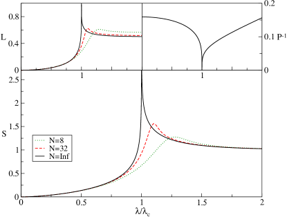
Figure 1: The von Neumann entropy $S$ between the atomic and bosonic modes for a range of system sizes, $N=8$, $N=32$, and $N\rightarrow\infty$. The divergence at $\lambda/\lambda_{c}=1$ can be clearly seen, as well as the strong coupling $S=1$ limit. The smaller graphs depict the linear entropy $S_{\text{lin}}$ between the atomic and bosonic modes Eq. (26), and the inverse participation ratio $P^{-1}$ Eq. (30) of the ground state wave-function. The linear entropy exhibits the similar behaviour to the von Neumann entropy, except the asymptotic limit changes with $N$ because of the normalisation. The participation ratio drops to $0$ at the critical point, indicating a massive delocalization of the ground state.

III.2 Thermodynamic limit

For $N\to\infty$, the excitation energy diverges as $\epsilon_{-}\propto|\lambda_{c}-\lambda|^{z\nu}$ and the characteristic length diverges as $l_{-}=\frac{1}{\sqrt{\epsilon_{-}}}\propto|\lambda-\lambda_{c}|^{-\nu}$ with the exponents $z=2$ and $\nu=1/4$ Emary202 . We now use the thermodynamic limit RDMs found above to obtain an exact analytical expression for the entropy $S$ as $N\rightarrow\infty$. This calculation proceeds via comparison with the density matrix of a single harmonic oscillator of mass $m$, frequency $\Omega$ at temperature $T$ Feynman98 ; Lambert04 with that of our reduced atomic system in Eq.(4). We find,

$$\cosh\beta\Omega = \left(1+\frac{2\epsilon_{-}\epsilon_{+}}{(\epsilon_{-}-\epsilon_{+})^{2}c^{2}s^{2}}\right),$$ (16)

$$m\Omega = \sqrt{\left(1+\frac{2\epsilon_{-}\epsilon_{+}}{(\epsilon_{-}-\epsilon+)^{2}c^{2}s^{2}}\right)^{2}-1}$$ (17)

$$\times \left(\frac{(\epsilon_{-}-\epsilon_{+})^{2}c^{2}s^{2}}{2\kappa^{2}(\epsilon_{-}c^{2}+\epsilon_{+}s^{2})}\right)$$

where $\beta=1/k_{B}T$. We have two equations linking the four parameters of the atomic RDM $\omega$, $\omega_{0}$, $\lambda$, $\kappa$ (where $\kappa$ is the squeezing parameter we introduced in Eq.(4)) and the three effective parameters of the thermal oscillator $\beta$, $\Omega$, $m$. By setting one energy scale of the original system such that $\omega_{0}=1$, and that of the thermal oscillator such that $m=1$, $\Omega=\omega$, we can uniquely define the correspondence between the two systems.

The squeezing parameter $\kappa$ introduced into the RDM in Eq. (4) compensates for the one-mode squeezing that the atomic ensemble undergoes as a function of $\lambda$ Emary02 , allowing us to keep the frequency of the thermal oscillator constant. With this relation between the parameters of the two RDMs, the effective temperature becomes the parameter describing the degree of mixing in the RDM. In other words, the interaction of the field with the atomic ensemble is such that, from the point of the atoms alone, it is as if they were at a finite temperature, with the temperature given by Eqs (17). The determination of this temperature is not unique, since there are more free parameters in Eqs (17) than constraints, but the choice made here is physically appealing, with the frequency of the thermal oscillator constant and the temperature varying with $\lambda$.

The behaviour of the temperature $T$ with $\lambda$ is shown in Fig. 2, and the divergence at the critical point is immediately obvious. We also plot the squeezing parameter $\kappa$, which vanishes at $\lambda_{c}$ in accordance with the delocalization of the system here.

The entropy of a harmonic oscillator at finite temperature is a standard result from statistical physics Feynman98 (setting $\hbar=k_{B}=1$),

$$S=\left(\frac{\Omega}{2T}\coth(\frac{\Omega}{2T})-\ln{(2\sinh(\frac{\Omega}{2T}))}\right)/\ln(2).$$ (18)

Note that this is independent of $\kappa$, and thus the above discussion does not affect the result for $S$. Solving Eqs (17) for the effective parameters, we obtain the von Neumann entropy of the atom-field system in the normal phase, which is plotted in Fig. 1. We clearly see a divergence at $\lambda_{c}$.

Moving into the SR phase, if we calculate the entropy of a single displaced lobe, exactly the same calculation as in the normal phase applies, except with the SR parameters instead of the normal phase ones. Around the critical point, the entropy diverges and then falls to zero for large coupling (not shown here). This is the correct scenario for $N\to\infty$, where parity symmetry is broken and the system sits in either of the displaced lobes.

The more interesting case occurs for large but finite $N$ where our numerical results indicate that for large coupling, the entropy $S$ does not tend to zero, but rather to a finite value. This can be easily understood by calculating the entropy of the positive-parity two-lobed SR RDM of Eq. (12), rather than the broken-parity single-lobe wave function as above. We recall that the two-lobe RDM for $N\gg 1$ formally turns out as a mixture of the density matrices representing each lobe, cf.  Eq. (12). A standard result Wehrl78 is that for a density matrix $\rho=\lambda_{1}\rho_{1}+\lambda_{2}\rho_{2}$, $\lambda_{1,2}\geq 0$, the concave nature of the von Neumann entropy allows us to write the following inequality,

$$S(\rho)\geq\lambda_{1}S(\rho_{1})+\lambda_{2}S(\rho_{2}).$$ (19)

The entropy of a mixture of density matrices is also bounded from above by

$$S(\rho)\leq\lambda_{1}S(\rho_{1})+\lambda_{2}S(\rho_{2})-\lambda_{1}\log\lambda_{1}-\lambda_{2}\log\lambda_{2}.$$ (20)

The final two terms are known as the mixing entropy Wehrl78 , and in the case that the ranges of the $\rho_{1}$ and $\rho_{2}$ are pairwise orthogonal, this upper bound becomes an equality. Returning to our positive-parity SR RDM, the entropy of each of the two lobes is identical $S(\rho_{1})=S(\rho_{2})$ and they are weighted in an equal superposition $\lambda_{1}=\lambda_{2}=1/2$. Furthermore, the two lobes are orthogonal, and thus from Eqs (19,20) we have

$$S(\rho)=S(\rho_{1})+1.$$ (21)

We emphasize that the SR phase entropy plotted in Fig.(1) is a consistent entanglement measure based on the underlying pure ground state  Eq. (11), yielding the correct large-$N$ behaviour for strong couplings $\lambda$.

From Eq. (18) we see the entropy depends only on the ratio $\Omega/T$. In the limit $\lambda\rightarrow\lambda_{c}$, we have $\Omega/T\sim\sqrt{\epsilon_{-}}$. Since as $\lambda\rightarrow\lambda_{c}$, $\epsilon_{-}\rightarrow 0$, we see that the effective temperature diverges $T\rightarrow\infty$ and so does the entropy, $S\rightarrow\infty$.

Figure 2: Effective entanglement temperature $T$ vs. $\lambda/\lambda_{c}$ for $N\rightarrow\infty$, $\omega=\omega_{0}=1$, from Eq. (16) with $\beta=1/T$. The divergence at the critical point causes the simultaneous divergence of the von Neumann entropy, signalling ‘maximal mixing’. The second graph illustrates the behaviour of the squeezing parameter $\kappa$ vs $\lambda/\lambda_{c}$ from Eq. (17), which tends to $0$ at the critical point.

As discussed in Lambert04 , in the neighbourhood of the critical point, we have

$$S_{\lambda\rightarrow\lambda_{c}} = [1-\frac{1}{4}\ln(\frac{64\lambda_{c}^{3}\omega^{4}}{16\lambda_{c}^{4}+\omega^{4}})-\frac{1}{4}\ln|\lambda_{c}-\lambda|]/\ln(2)$$ (22)

$$= -\frac{1}{4}\log_{2}|\lambda_{c}-\lambda|+\text{const}.$$

The prefactor to the logarithmic divergence is identical to the exponent characterising the divergence of the length scale $\nu=1/4$. Thus we see that, as adjudged by the atom-field entropy, the system is critically entangled.

III.3 Linear Entropy, Participation Ratio, and the Average Linear Entropy

An alternative measure of entanglement is the linear entropy, given by

$$L=\eta[1-\text{Tr}(\rho^{2})],$$ (23)

where $\rho$ is the reduced density matrix of one part of our bipartite system, and $\eta$ is the normalisation $\eta=1+(1/N)$ which gives the correct $0\leq L\leq 1$ behaviour sco04 . While it is a valid monotonic entanglement measure, it lacks some of the full physical interpretation provided by the von Neumann entropy Schumacher93 ; Bennett96 . Again, we calculate explicit analytical expressions in the thermodynamic limit by employing our co-ordinate space ground state (noting for $D\rightarrow\infty$, $\eta\rightarrow 1$),

$$\text{Tr}(\rho^{2}) = \int dxdx^{\prime}\rho(x,x^{\prime})\rho(x^{\prime},x)$$

$$= \int dxdx^{\prime}dydy^{\prime}\psi(x,y)\psi(x^{\prime},y)\psi(x,y^{\prime})\psi(x^{\prime},y^{\prime}).$$

In the normal phase

$$L = 1-\left(\frac{\epsilon_{-}\epsilon_{+}}{(\epsilon_{-}c^{2}+\epsilon_{+}s^{2})}\right)[(\epsilon_{-}s^{2}+\epsilon_{+}c^{2})^{2}$$

$$- \frac{(\epsilon_{-}s^{2}+\epsilon_{+}c^{2})(\epsilon_{-}-\epsilon_{+})^{2}c^{2}s^{2}}{(\epsilon_{-}c^{2}+\epsilon_{+}s^{2})}]^{-1/2},$$

On resonance when $\omega=\omega_{0}=1,c=s=1/\sqrt{2}$ this simplifies to

$$L=1-\frac{2\sqrt{\epsilon_{-}\epsilon_{+}}}{(\epsilon_{-}+\epsilon_{+})},$$ (26)

which is zero at zero coupling, and unity at the critical point. In the SR phase we recall the ground state (for large but finite $N$) is a superposition of two lobes, and the RDM is a mixture, thus,

$$\text{Tr}(\rho^{2})=\frac{1}{4}(\text{Tr}(\rho_{1}^{2})+\text{Tr}(\rho_{2}^{2})+2\text{Tr}(\rho_{1}\rho_{2})).$$ (27)

As before, the two lobes are pairwise orthogonal, $\text{Tr}(\rho_{1}^{2})=\text{Tr}(\rho_{2}^{2})$, and the cross term is zero. Therefore, we need

$$L=1-\frac{1}{2}\text{Tr}(\rho_{1}^{2}).$$ (28)

The explicit expression for this is the same as in the normal phase, but with the above factor $1/2$, and the appropriate SR parameters. In the large coupling limit, $\text{Tr}(\rho_{1}^{2})=1$, and thus the linear entropy tends to a constant $1/2$. This function, and the finite numerics, are shown in one of the insets of Fig. 1.

III.3.1 Inverse Participation Ratio

There is also a connection between the linear entropy, and the inverse participation ratio Edwards72 , a measure of the delocalization of a wave function. The un-normalised inverse participation ratio is defined as,

$$P^{-1}=\int dxdy|\Psi^{4}(x,y)|,$$ (29)

Typically, this is normalised over the volume of the co-ordinate space, however we work with the un-normalised value for convenience. $P^{-1}\rightarrow 0$ for a state delocalized across the entire co-ordinate space, and $P^{-1}$ remains finite for a localised state, depending on the basis chosen.

We can interpret the participation ratio as a measure of the spread of a wave function over a particular basis, akin to the way the entropy is a measure of the spread of a density matrix over its diagonal basis. In the normal phase, we perform the Gaussian integrals with respect to the spin-boson co-ordinates to obtain

$$P^{-1}=\frac{\sqrt{\epsilon_{-}\epsilon_{+}}}{2\pi}.$$ (30)

Thus, in this representation, the participation ratio is equal to the Gaussian normalisation factor of the ground state, telling us the relative volume in co-ordinate space the state occupies.

In the SR phase, $\Psi^{\text{SR}}_{G}|_{N\gg 1}=\frac{1}{\sqrt{2}}(\psi_{1}+\psi_{2})$, where $\psi_{1,2}$ represents the two possible displaced lobes. Again, using the fact that there is no overlap between these lobes, we see,

$$P^{-1}=\int dxdy\frac{1}{4}(\psi_{1}^{4}+\psi_{2}^{4})=\int dxdy\frac{1}{2}\psi_{1}^{4}(x,y),$$ (31)

thus yet again we can use the normal phase result, with the SR phase parameters. This analytical result is plotted in Fig. 1, where the delocalization at the critical point is clearly shown.

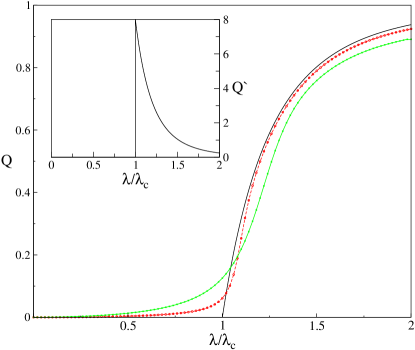
Figure 3: The average linear entropy for system sizes $N=8$, $N=16$, and $N\rightarrow\infty$ Eq. (III.3.2) which includes contributions from both the field and atomic modes. Inset: The derivative of the $N\rightarrow\infty$ limit.

III.3.2 Average Linear Entropy

To conclude our discussion, we define the average linear entropy over all subsystems ($N$–atoms and the field mode) as,

$$Q \equiv \left[\frac{1}{N+1}[\sum_{k=0}^{N-1}L_{k}+L_{b}]\right]=\frac{N}{N+1}L_{k}+\frac{1}{N+1}(L_{b}),$$

where the sum is replaced because the Dicke states are symmetric with respect to interchange of atoms. $L_{k}$ is the linear entropy of atom $k$, and $L_{b}$ is the linear entropy of the mode discussed earlier,

$$L_{k} = \eta_{2}(1-\text{Tr}(\rho_{k}^{2})),\quad L_{b}=\eta_{N+1}(1-\text{Tr}(\rho_{b}^{2})).$$ (32)

As before in Eq.(23), the quantities $\eta_{2}=2$ and $\eta_{N+1}=1+(1/N)$ provide the correct normalisation. Since the linear entropy of one subsystem of a pure state is an entanglement monotone Emary04 (it does not increase under local operations and classical communication), and a valid entanglement measure, a concave function of the linear entropy is also an entanglement monotone. The average linear entropy $Q$, as we have defined it here, is a concave function, and is thus itself an entanglement monotone.

We can express $\rho_{k}$, the reduced density matrix of any atom from the ensemble, in terms of the collective expectation values,

$$\rho_{k}=\left[\begin{array}[]{cc}\frac{1}{2}(1-\frac{2\langle J_{z}\rangle}{N})&\frac{\langle J_{-}\rangle}{N}\\ \frac{\langle J_{+}\rangle}{N}&\frac{1}{2}(1+\frac{2\langle J_{z}\rangle}{N})\end{array}\right],$$ (35)

and we find $\text{Tr}(\rho_{k}^{2})=\frac{1}{2}+\frac{2\langle J_{z}\rangle^{2}}{N^{2}}+\frac{2\langle J_{-}\rangle\langle J_{+}\rangle}{N^{2}}$. Thus, the linear entropy of a single atom is,

$$L_{k}=1-4\langle J_{z}\rangle^{2}/N^{2}.$$ (36)

In the thermodynamic limit, $\langle J_{z}\rangle^{2}=\langle b^{\dagger}b\rangle^{2}-N\langle b^{\dagger}b\rangle+N^{2}/4$, and we have $L_{k,N\rightarrow\infty}^{\lambda<\lambda_{c}}=0$. In the super-radiant phase, $\langle J_{z}\rangle^{2}=\langle d^{\dagger}d\rangle^{2}-N\mu\langle d^{\dagger}d\rangle+N^{2}\mu^{2}/4$, and thus $L_{k,N\rightarrow\infty}^{\lambda>\lambda_{c}}=(1-\mu^{2})$, ($\mu=\lambda_{c}^{2}/\lambda$). In both phases the contribution from the mode becomes negligible, and $Q_{N\rightarrow\infty}=L_{k}$. Numerical results for this quantity are plotted in Fig. (3).

It has been shown elsewhere Brennen03 that the average linear entropy $Q$ is related to a measure of multipartite entanglement proposed by Meyer and Wallach Meyer01 . The concept of multipartite entanglement is a difficult and open one (e.g.lin99 ; Cart99 ; miy03 ; ver03 ), and while the average linear entropy is limited in the multipartite states it can classify Emary04 it is both easy to calculate and has proved useful in a variety of contexts contexts sco04 ; Brennen03 ; Scott03 ; Somma04 . For completeness, we provide a definition of Meyer and Wallach’s measure in the appendix.

In our results Fig.(3), we see a clear discontinuity in $Q$ between the two phases. This follows directly from the discontinuity of the atomic inversion at the critical point Emary02 , and the simple nature of our symmetric atomic states. As a final point, the derivative of $Q$ in the SR phase TD limit is $\frac{\partial Q}{\partial\lambda}=4\lambda_{c}^{4}/\lambda^{5}$, which we plot as an inset in Fig. (3). In the thermodynamic limit the average entanglement of all the physical subsystems vanishes in the normal phase, but becomes non-zero in the superradiant phase. However, the maximum of $Q$ is not at the critical point, contrary to the bipartite partitions and the pairwise partitions Lambert04 .

IV Discussion and Conclusions

Table 1 presents the most important results for the entanglement measures we have calculated here (and the concurrence discussed in Lambert04 ), and where appropriate their derivatives. In particular, we point out the importance of the divergences at the critical point, and the finite size scaling exponents (not discussed here) we calculated in Lambert04 , and which have been recently confirmed in Reslen04 .

$f(\lambda)$	$f(\lambda\rightarrow\lambda_{c})$	$N$ Scaling
$\epsilon_{-}$	$|\lambda_{c}-\lambda|^{1/2}$	-
$l_{-}$	$|\lambda_{c}-\lambda|^{-1/4}$	-
S	$-\frac{1}{4}\log_{2}|\lambda-\lambda_{c}|$	$\log_{2}N^{(0.14\pm 0.01)}$
$C_{R}$	$1-\frac{\sqrt{2}}{2}$	$N^{-0.25\pm 0.01}$
$\frac{\partial C_{R}}{\partial\lambda}$	$|\lambda_{c}-\lambda|^{-\frac{1}{2}}$	-

Table 1: Entropy $S$, Eq. (18), concurrence $C_{R}$ (from Lambert04 ), and the average linear entropy Eq. (36), in the Dicke model near the critical point $\lambda\rightarrow\lambda_{c}$.

For the atom-boson partition, we calculated the entropy exactly in the thermodynamic limit and numerically for finite $N$. The entropy has a divergence around $\lambda=\lambda_{c}$, which follows the power law divergence of the correlation length $l_{-}\propto|\lambda-\lambda_{c}|^{-1/4}$.

There is also a correspondence between the divergence of the spin-boson entanglement (entropy) and the delocalization of the wave function. This is highlighted by our results for the behaviour of the participation ratio, which shows that the ground state of the Dicke model undergoes a massive delocalization at the critical point. Since delocalization is a common property of wave functions in a quantum chaotic system, our results help strengthen the understanding of the relationship between entanglement and the underlying integrable to chaotic transition present in the Dicke Hamiltonian Emary02 . However, most generic features of this relationship are still unknown. The future of this field lies in closer examination of the underlying semi-classical behaviour in quantum systems, such as supercritical pitchfork bifurcations Hines03 in co-ordinate space, or phase space.

Similarly, we calculated the average linear entropy, and example of the Meyer-Wallach multipartite entanglement. Like our other measures, this displays a clear discontinuity at the critical point. There is obvious future research to be done in applying the many larger classes of multipartite entanglement measures Emary04 in a compact way, and perhaps gaining a clearer understanding of the behaviour of multipartite entanglement. Other avenues of future research may arise from investigating quantum phase transitions in other spin-boson models Emary02 ; Hines03 . In particular, while the Dicke model has a natural feature that allows infinite system sizes to be investigated, there is no reason other spin-boson models with non-commuting energy and interaction terms which do not have this integrable limit should not exhibit similar critical entanglement, with chaotic transitions and level statistics.

Appendix A Meyer-Wallach Entanglement

Here we include the definition of the Meyer-Wallach entanglement measure Meyer01 , as originally intended for a system of $N$–qubits, and show its connection to the average linear entropy.

We can write the pure state of $N$ qubits as $|\psi\rangle=\sum_{b_{1},...,b_{N}}a_{b_{1},...,b_{N}}|b_{1},...,b_{N}\rangle$. Meyer and Wallach defined two new unnormalised states $|\tilde{u}^{k}\rangle$ and $|\tilde{v}^{k}\rangle$ as vectors in $C^{2N-1}$ which are obtained by projecting the original state $|\psi\rangle$ onto the two possible subspaces spanned by the two possible states of the $k-\text{th}$ qubit,

$$|\psi\rangle=|0\rangle_{k}\otimes|\tilde{u}^{k}\rangle+|1\rangle_{k}\otimes|\tilde{v}^{k}\rangle.$$ (37)

In the Schmidt decomposition, these two subspaces are orthogonal $\langle\tilde{u}^{k}|\tilde{v}^{k}\rangle=0$. $Q$ itself is defined as,

$$Q(|\psi\rangle)=\frac{4}{N}\sum_{k=1}^{N}D(|\tilde{u}^{k}\rangle,|\tilde{v}^{k}\rangle)$$ (38)

where $D(|\tilde{u}^{k}\rangle,|\tilde{v}^{k}\rangle)=\sum_{i\leq j}|\tilde{u}^{k}_{i}\tilde{v}^{k}_{j}-\tilde{u}^{k}_{j}\tilde{v}^{k}_{i}|^{2}$ is the generalised wedge product.

Brennen proved that each term $D$ in the sum of $Q$ was equal to the linear entropy of the $k$th qubit, and thus $Q(|\psi\rangle)$ is equivalent to the average linear entropy of all the qubits,

$$Q(|\psi\rangle)=2\left[1-\frac{1}{N}\sum_{k=0}^{N-1}\text{Tr}(\rho_{k}^{2})\right],$$ (39)

where $\rho_{k}$ is the reduced density matrix of the $k$th qubit. Thus, $Q$ has the required properties of an entanglement measure $0\leq Q(|\psi\rangle)\leq 1$, $Q(|\psi\rangle)=0$ for product states, $Q(|\psi\rangle)=1$ for the reduced density matrix of every qubit being maximally mixed, and $Q(|\psi\rangle)$ is invariant under local unitaries, both because $D$ is invariant, and $\text{Tr}(\rho_{k}^{2})$ is invariant.

Many pure states fulfil the requirement for maximal qubit mixing, and thus give a value of $Q=1$. For example, the 3-qubit GHZ state $(|000\rangle+|111\rangle)/\sqrt{2}$ gives $Q=1$, while the Werner state gives $Q((|100\rangle+|010\rangle+|001\rangle)/\sqrt{3})=\frac{8}{9}$.

References

- (1) S. Sachdev Quantum Phase Transitions, (Cambridge University Press, 1999).
- (2) M. C. Gutzwiller, Chaos in Classical and Quantum Mechanics, (Springer, 1990).
- (3) T. J. Osborne and M. A. Nielsen, Phys. Rev. A 66, 032110 (2002).
- (4) A. Osterloh, L. Amico, G. Falci, R. Fazio, Nature 416, 608 (2002).
- (5) G. Vidal, J. I. Latorre, E. Rico, and A. Kitaev, Phys. Rev. Lett. 90, 227902.
- (6) J. I. Latorre, E. Rico, and G. Vidal, Quant. Inf. and Comp. 4, 1 (2004).
- (7) M. Srednicki, Phys. Rev. Lett. 71, 666 (1993).
- (8) J.I. Latorre and R. Orús, Phys. Rev. A 69, 062302 (2004).
- (9) J. Vidal, G. Palacios, and R. Mosseri, Phys. Rev. A 69, 022107 (2004).
- (10) N. Lambert, C. Emary and T. Brandes, Phys. Rev. Lett. 92, 073602 (2004).
- (11) A. Wehrl, Rev. Mod. Phys. 50, 221 (1978).
- (12) B. Schumacher, Phys. Rev. A 51, 2738 (1993).
- (13) D. A. Meyer and N. R. Wallach, quant-ph/0108104
- (14) C. Emary and T. Brandes, Phys Rev. Lett. 90, 044101 (2003).
- (15) C. Emary and T. Brandes, Phys. Rev. E 67, 066203 (2003).
- (16) A. P. Hines, G.J. Milburn, and R. H. McKenzie, quant-ph/0308165.
- (17) S. Schneider, and G. J. Milburn, Phys. Rev. A 65, 042107 (2002).
- (18) H. Fujisaki, T. Miyadera, and A. Tanaka, Phys. Rev. E 67, 066201 (2003).
- (19) T. Vorrath and T. Brandes, Phys. Rev. B 68, 035309 (2003).
- (20) X. Wang and K. Mølmer, Eur. Phys. J. D 18, 385 (2002).
- (21) X. Wang, M. Feng, and B. C. Sanders, Phys. Rev. A 67, 022302 (2003)
- (22) M. B. Plenio and S. F. Huelga, Phys. Rev. Lett. 88, 197901 (2002).
- (23) T. Brandes and N. Lambert, Phys. Rev. B 67, 125323 (2003).
- (24) J. Reslen, L. Quiroga, and N. F. Johnson, cond-mat/0406674
- (25) C. Emary, PhD Thesis, UMIST, Manchester (UK), unpublished (2001).
- (26) M. Frasca, Ann. Phys. 313 26 (2004).
- (27) R. P. Feynman, Statistical Mechanics (The Perseus Books Group, 1998).
- (28) A. J. Scott, Phys. Rev. A 69, 052330 (2004).
- (29) C. H. Bennett, D. P. DiVincenzo, J. A. Smolin, and W. K. Wootters, Phys. Rev. A. 54, 3824 (1996).
- (30) J. T. Edwards and D. J. Thouless, J. Phys. C: Solid State Phys 5, 8 (1972).
- (31) C. Emary, quant-ph/0405049
- (32) G. K. Brennen, Quantum Information and Computation 3, 619 (2003).
- (33) N. Linden, S. Popescu, and A. Sudbery, Phys. Rev. Lett. 83, 243 (1999).
- (34) H. A. Carteret, N. Linden, S. Popescu, and A. Sudbery, Found. Phys. 29, 527 (1999).
- (35) A. Miyake, Phys. Rev. A 67, 012108 (2003).
- (36) F. Verstraete, J. Dehaene, and B. De Moor, Phys. Rev. A 68, 012103 (2003).
- (37) R. Somma, G. Ortiz, H. Barnum, E. Knill, and L. Viola, Phys. Rev. A 70, 042311 (2004).
- (38) A. J. Scott and C. M. Caves, J. Phys. A 36, 9553 (2003).