Some useful combinatorial formulae for bosonic operators

Abstract

We give a general expression for the normally ordered form of a function $F[\hat{w}(a,a^{\dagger})]$ where $\hat{w}$ is a function of boson creation and annihilation operators satisfying $[a,a^{\dagger}]=1$. The expectation value of this expression in a coherent state becomes an exact generating function of Feynman-type graphs associated with the zero-dimensional Quantum Field Theory defined by $F(\hat{w})$. This enables one to enumerate explicitly the graphs of given order in the realm of combinatorially defined sequences. We give several examples of the use of this technique, including the applications to Kerr-type and superfluidity-type hamiltonians.

In the normally ordered form of a function $F(a,a^{\dagger})$ of boson creation and annihilation operators all the annihilation operators are moved to the right using the commutation relation $[a,a^{\dagger}]=1$. The importance of the normal form, denoted by $\mathcal{N}[F(a,a^{\dagger})]$ and satisfying $F(a,a^{\dagger})=\mathcal{N}[F(a,a^{\dagger})]$, is evident, as with it the expectation values of $F(a,a^{\dagger})$ can be easily evaluated in such canonical states as the vacuum $|0\rangle$ and coherent states $|z\rangle=e^{-|z|^{2}/2}\sum_{n=0}^{\infty}z^{n}/\sqrt{n!}\ |n\rangle$, ($z$ complex and $a^{\dagger}a|n\rangle=n|n\rangle$). The role of the normal form in Quantum Field Theory (QFT) is pre-eminent [1, 2].

In this work we consider functions $F(\hat{w})$ that involve operators $\hat{w}(a,a^{\dagger})$ in the form of a product of positive powers of $a^{\dagger}$ and $a$, and powers of $(a+a^{\dagger})$, although the formulae derived below are valid for more general $\hat{w}$’s. Our considerations are based on the following operational property of formal power series. Let $f(x)=\sum_{n=0}^{\infty}f_{n}x^{n}/n!$ and $g(x)=\sum_{n=0}^{\infty}g_{n}x^{n}/n!$ be two formal power series, also called the exponential generating functions (egf) of sequences $\{f_{n}\}_{n=0}^{\infty}$ and $\{g_{n}\}_{n=0}^{\infty}$, respectively. Then it can be verified that

$$\left.f\left(\lambda\frac{d}{dx}\right)g(x)\right|_{x=0}=\left.g\left(\lambda\frac{d}{dx}\right)f(x)\right|_{x=0}=\sum_{n=0}^{\infty}f_{n}\cdot g_{n}\ \frac{\lambda^{n}}{n!},$$

which we shall call the product formula (PF). This implies the following property satisfied by $F(\lambda\hat{w})$ with indeterminate $\lambda$:

$$F(\lambda\hat{w})=\left.F\left(\lambda\frac{d}{dx}\right)e^{x\hat{w}}\right|_{x=0},$$ (1)

which by taking the normal form of both sides becomes

$$\mathcal{N}[F(\lambda\hat{w})]=\left.F\left(\lambda\frac{d}{dx}\right)\mathcal{N}(e^{x\hat{w}})\right|_{x=0}.$$ (2)

Note that in Eq.(2) a separation has been achieved between the functional aspect (defined by $F$) and the operator aspect (defined by $\hat{w}$) of the normal ordering. Conventionally we implement $\mathcal{N}(e^{x\hat{w}})$ by using the auxiliary symbol $:\ :$ with $\mathcal{N}(e^{x\hat{w}})\equiv\ :G_{\hat{w}}(x,a,a^{\dagger}):$ , where under the symbol $:\ :$ the function $G_{\hat{w}}(x,a,a^{\dagger})$ is normally ordered assuming that $a^{\dagger}$ and $a$ commute [3, 4]. Then Eq.(2) becomes

$$\mathcal{N}[F(\lambda\hat{w})]=\left.F\left(\lambda\frac{d}{dx}\right):G_{\hat{w}}(x,a,a^{\dagger}):\right|_{x=0}.$$ (3)

Note that the expression of Eq.(3) arises in the evaluation of the partition function $Z_{\beta}$ for the system defined by the hamiltonian $\mathcal{H}(\hat{w})$

$$Z_{\beta}={\textnormal{Tr}}\ e^{-\beta\mathcal{H}(\hat{w})}=\frac{1}{\pi}\int d^{2}z\left[\left.e^{-\beta\mathcal{H}\left(\frac{d}{dx}\right)}G_{\hat{w}}(x,z,z^{*})\right|_{x=0}\right],$$

taking the trace over the coherent state representation, $\beta=(k_{B}T)^{-1}$ [5]. The problem of finding $\mathcal{N}[F(\lambda\hat{w})]$ reduces to that of finding $\mathcal{N}(e^{x\hat{w}})$, still however a non-trivial task, vide the classical references [3, 4, 6]. We have recently found expressions for $G_{\hat{w}}(x,a,a^{\dagger})$ for several types of operators $\hat{w}$ of the form $\hat{w}_{(r,s)}=(a^{\dagger})^{r}a^{s}$ [7] as well as for $\hat{w}_{(\vec{r},\vec{s})}=\prod_{k=1}^{M}\hat{w}_{(r_{k},s_{k})}$ with $r,s,r_{k},s_{k}$ positive integers [8].

At this point it is already possible to relate Eq.(3) to enumerative formulae for Feynman-like graphs in QFT [9]. Assume that our formal power series $F(x)$ can be written in the form $F(x)=\exp\left(\sum_{m=1}^{\infty}L_{m}\frac{x^{m}}{m!}\right)$, and we similarly assume that we may define operators $V_{n}^{(\hat{w})}(a,a^{\dagger})$ by

$$:G_{\hat{w}}(x,a,a^{\dagger}):=\ :\exp\left(\sum_{n=1}^{\infty}V_{n}^{(\hat{w})}(a,a^{\dagger})\frac{x^{n}}{n!}\right):\ .$$ (4)

Explicit examples [7] from which the operators $V_{n}^{(\hat{w})}(a,a^{\dagger})$ may be read off include:

$$\begin{array}[]{rcl}\hat{w}=a^{\dagger}a,&&\mathcal{N}[\exp\left(xa^{\dagger}a\right)]=\ :\exp\left[a^{\dagger}a(e^{x}-1)\right]:\ ,\end{array}$$ (5)

$$\begin{array}[]{rcl}\hat{w}=(a^{\dagger})^{r}a,&&\mathcal{N}[\exp\left(x(a^{\dagger})^{r}a\right)]=\\ &&=\ :\exp\left[a^{\dagger}a\sum_{n=1}^{\infty}(a^{\dagger})^{(r-1)n}(r-1)^{n}\frac{\Gamma(n+\frac{1}{r-1})}{\Gamma(\frac{1}{r-1})}\frac{x^{n}}{n!}\right]:\end{array}$$ (6)

with $r=2,3\ldots$ , as well as more involved expressions for other $\hat{w}(a,a^{\dagger})$. Thus, Eq.(3) may be written as

$$\begin{array}[]{c}\mathcal{N}[F(\lambda\hat{w})]=\exp\left(\sum_{m=1}^{\infty}\frac{L_{m}}{m!}\lambda^{m}\frac{d^{m}}{dx^{m}}\right)\cdot\left.:\exp\left(\sum_{n=1}^{\infty}V_{n}^{(\hat{w})}(a,a^{\dagger})\frac{x^{n}}{n!}\right):\ \right|_{x=0}.\end{array}$$ (7)

We eliminate the operators $a$ and $a^{\dagger}$ by taking the matrix element of Eq.(7) in the coherent state $|z\rangle$ and using $a|z\rangle=z|z\rangle$. This yields

$$\begin{array}[]{c}\langle z|\mathcal{N}[F(\lambda\hat{w})]|z\rangle=\left.\exp\left(\sum_{m=1}^{\infty}\frac{L_{m}}{m!}\lambda^{m}\frac{d^{m}}{dx^{m}}\right)\cdot\right.\left.\exp\left(\sum_{n=1}^{\infty}V_{n}^{(\hat{w})}(z,z^{*})\frac{x^{n}}{n!}\right)\right|_{x=0}.\end{array}$$ (8)

By specifying $z=1$ in Eq.(8), defining $V_{n}^{(\hat{w})}(1,1)=V_{n}^{(\hat{w})}$, $\mathbf{V}=\{V_{n}^{(\hat{w})}\}_{n=1}^{\infty}$ and $\mathbf{L}=\{L_{m}\}_{m=1}^{\infty}$ we obtain

$$Z(\mathbf{L},\mathbf{V},\lambda)\equiv\langle 1|\mathcal{N}[F(\lambda\hat{w})]|1\rangle$$

$$=\left.\exp\left(\sum_{m=1}^{\infty}\frac{L_{m}}{m!}\lambda^{m}\frac{d^{m}}{dx^{m}}\right)\right.\left.\cdot\exp\left(\sum_{n=1}^{\infty}V_{n}^{(\hat{w})}\frac{x^{n}}{n!}\right)\right|_{x=0}$$ (9)

which is essentially the counting formula cited by Bender et al. [9]. Due to the symmetry of the PF , we have $Z(\mathbf{L},\mathbf{V},\lambda)=Z(\mathbf{V},\mathbf{L},\lambda)$, which may facilitate the calculations. Furthermore it can be demonstrated that for all the forms of $\hat{w}$ used here the sequence $\mathbf{V}$ consists of positive integers. The formula Eq.(9) was employed in [9] as an enumerative tool for counting the Feynman-like graphs in zero-dimensional QFT models, where the values of all Feynman integrals are equal to one. Our derivation sheds light on its quantum origin by tracing back its sources to the boson normal ordering problem. By specifying the sets $\mathbf{L}$ and $\mathbf{V}$ one can attempt to produce a (in general divergent) power series expansion in $\lambda$:

$$Z(\mathbf{L},\mathbf{V},\lambda)=\sum_{n=0}^{\infty}A_{n}(\mathbf{L},\mathbf{V})\frac{\lambda^{n}}{n!}\$$ (10)

in which $A_{n}(\mathbf{L},\mathbf{V})$ can be related to known objects. To see that, recall the definition of the multivariate Bell polynomials $\mathbb{B}(\mathbf{h},u)$ related to a function $h(x)=\sum_{n=1}^{\infty}h_{n}\frac{x^{n}}{n!}$ through ($\mathbf{h}=\{h_{n}\}_{n=1}^{\infty}$)

$$e^{uh(x)}=\sum_{n=0}^{\infty}\frac{x^{n}}{n!}\sum_{k=1}^{n}u^{k}\mathbb{B}_{nk}(\mathbf{h})=\sum_{n=0}^{\infty}\frac{x^{n}}{n!}\mathbb{B}_{n}(\mathbf{h},u),$$ (11)

where the coefficients of the expansion $\mathbb{B}_{n}(\mathbf{h},u)=\sum_{k=1}^{n}u^{k}\mathbb{B}_{nk}(\mathbf{h})$ depend only on $h_{1},\ldots,h_{n}$. We refer to [10, 11] for further properties of $\mathbb{B}_{n}(\mathbf{h},u)$.

With $\mathbb{B}_{n}(\mathbf{f})=\mathbb{B}_{n}(\mathbf{f},1)$ we see that the coefficients $A_{n}=A_{n}(\mathbf{L},\mathbf{V})$ factorize

$$A_{n}=\mathbb{B}_{n}(\mathbf{L})\cdot\mathbb{B}_{n}(\mathbf{V})$$ (12)

which for given $\mathbf{L}$ and $\mathbf{V}$ can be worked out (see below).

The utility of Eqs.(9) and (12) goes beyond the specific definition of initial $\hat{w}$, and this is the philosophy of Ref.[9] where it was suggested that $\mathbf{L}$ and $\mathbf{V}$ could be treated as initial input for QFT models. From this perspective Eqs.(9) and (12) provide the starting point for a Feynman-like graph representation of the coefficients $A_{n}$ in Eq.(10), where $A_{n}$ counts the number of graphs with $n$ labelled lines. The graph construction rules are: a line starts from a white dot, the origin, and ends at a black dot, the vertex. We further associate strengths $V_{k}$ with each vertex receiving $k$ lines and multipliers $L_{m}$ with a white dot which is the origin of $m$ lines. Counting such graphs consists in calculating their multiplicity due to the labelling of lines and the factors $L_{m}$ and $V_{k}$.

We now specify $\mathbf{L}$ and $\mathbf{V}$ and give some examples of the explicit evaluation of $A_{n}$ along with the explicit graph representation:

Example 1: $L_{1}=1$, $L_{M}=1$ ($M>1$), and $L_{m}=0$ otherwise, giving the function $F(x)=\exp(x+x^{M}/M!)$; $V_{n}^{(\hat{w})}=1$ for $n=1,2\ldots$, which arises from the string $\hat{w}=a^{\dagger}a$, see Eq.(5). This corresponds to the normal ordering problem $\mathcal{N}[\exp(\lambda a^{\dagger}a+\frac{\lambda^{M}}{M!}(a^{\dagger}a)^{M})]$. Note that the case $M=2$ describes the normal ordering of the exponential of the Kerr-type hamiltonian [12] $\mathcal{H}=\lambda a^{\dagger}a(1+\frac{\lambda}{2}a^{\dagger}a)$. Using the definition of the two variable Hermite-Kampé de Fériet polynomials $H_{n}^{(M)}(x,y)$ (see [13] and references therein)

$$\sum_{n=0}^{\infty}H_{n}^{(M)}(x,y)\frac{t^{n}}{n!}=e^{xt+yt^{M}},$$ (13)

where $H_{n}^{(M)}(x,y)=n!\sum_{r=0}^{[n/M]}\frac{x^{n-Mr}y^{r}}{(n-Mr)!r!}$, $F(x)$ can be expanded as

$$F(x)=e^{x+\frac{x^{M}}{M!}}=\sum_{n=0}^{\infty}H_{n}^{(M)}(1,\frac{1}{M!})\frac{x^{n}}{n!}.$$ (14)

Eq.(10) yields $A_{n}=H_{n}^{(M)}\left(1,\frac{1}{M!}\right)\cdot B_{n}$, where the Bell numbers $B_{n}$ are defined through their egf: $\exp(e^{x}-1)=\sum_{n=0}^{\infty}B_{n}\frac{x^{n}}{n!}$ [9, 10, 11]. Observe that for $M=2$, $H_{n}^{(2)}(1,\frac{1}{2})=\left(\frac{i}{\sqrt{2}}\right)^{n}H_{n}\left(-\frac{i}{\sqrt{2}}\right)=1,2,4,10,26,76,232,...$ are the involution numbers [10] expressible using Hermite polynomials $H_{n}(x)$. The initial terms of $A_{n}$ for $M=2$ are: $1,4,20,150,1352,15428,...$, see Fig.(1), and for $M=3$: $1,2,10,75,527,6293,...$, etc. Note that whereas $B_{n}$ counts all the partitions of an $n$-set, $H_{n}^{(M)}(1,\frac{1}{M!})$ counts partitions of an $n$-set into singletons and $M$-tons.

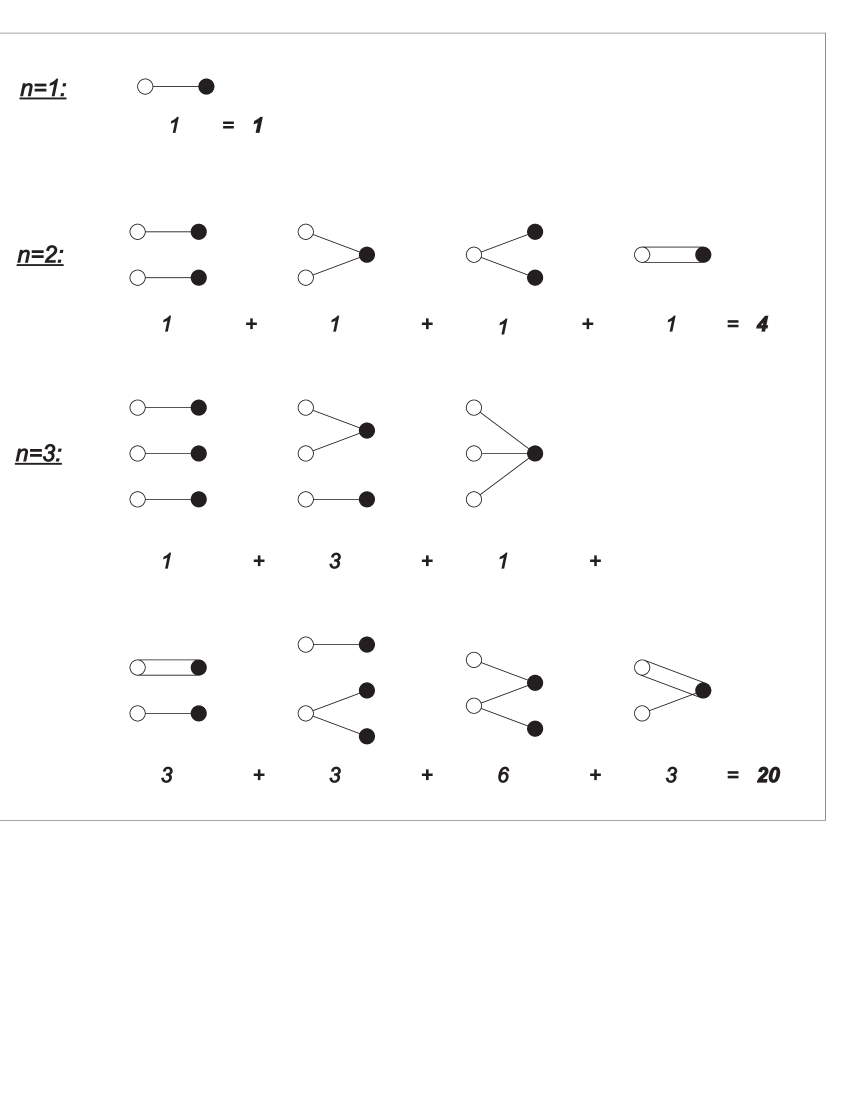
Figure 1: Lowest order Feynman-type graphs for Example 1 with $n=1,2,3$ lines. The number below each graph is its multiplicity.

Example 2: $L_{m}=m$ for $m=1,2\ldots$ , giving rise to $F(x)=\exp(\sum_{m=1}^{\infty}{\scriptstyle m}\frac{x^{m}}{m!})=\exp(xe^{x})=\sum_{n=0}^{\infty}I_{n}\frac{x^{n}}{n!}$, where $I_{n}=\sum_{k=0}^{\infty}\left(\!\!\!\!\!\stackrel{{{}^{\ }_{\ }}}{{{}^{\ }}}\right.\begin{array}[]{c}n\\ k\end{array}\left.\!\!\!\!\!\stackrel{{{}^{\ }_{\ }}}{{{}^{\ }}}\right)k^{n-k}$ are idempotent numbers [10]. Again choosing $V_{n}^{(\hat{w})}=1$, $n=1,2\ldots$, with $\hat{w}=a^{\dagger}a$, gives $A_{n}=I_{n}\cdot B_{n}=1,6,50,615,10192,214571\ldots$  . This corresponds to normally ordering $\mathcal{N}[\exp(\lambda(a^{\dagger}a)e^{\lambda(a^{\dagger}a)})]$.

Example 3: $L_{1}=0$, $L_{m}=1$ for $m=2,3\ldots$ , leading to $F(x)=\exp(e^{x}-1-x)=\sum_{n=0}^{\infty}B_{n}^{(1)}\frac{x^{n}}{n!}$, where $B_{n}^{(1)}$ are restricted Bell numbers which are defined as counting partitions without singletons. (Note that $B^{(1)}_{n}=\frac{1}{e}\sum_{k=0}^{\infty}\frac{(k-1)^{n}}{k!}$). Here we choose $V_{n}^{(\hat{w})}=n!$, $n=1,2\ldots$ , derived from the string $\hat{w}=(a^{\dagger})^{2}a$, and producing via $\exp\left(\frac{x}{1-x}\right)=\sum_{n=0}^{\infty}B_{n}^{(2,1)}\frac{x^{n}}{n!}$, (see Eq.(37) of [7]), $A_{n}=B_{n}^{(1)}\cdot B_{n}^{(2,1)}=0,3,13,292,5511,166091\ldots$, see Fig.(2). This corresponds to the normal ordering of $\exp\left(e^{\lambda(a^{\dagger})^{2}a}-1-\lambda(a^{\dagger})^{2}a\right)$.

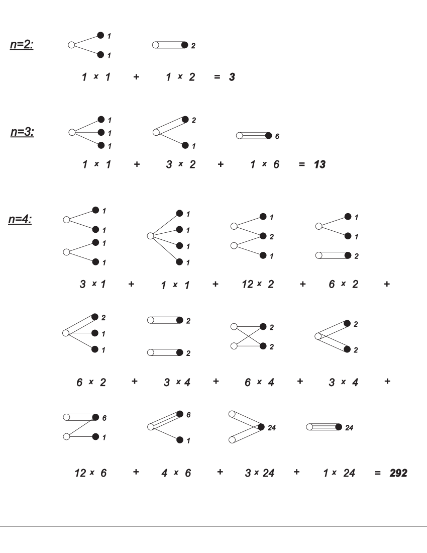
Figure 2: Lowest order Feynman-type graphs for Example 3 with $n=2,3,4$ lines. The number below each graph is $(multiplicity)\times\prod_{k}(vertex\ factor\ V_{k}=k!)$. Numbers at black dots (vertices) are vertex factors.

Example 4: $L_{2m}=2m,\ L_{2m+1}=0$ for $m=0,1,2\ldots$ , giving $F(x)=\exp(x\sinh(x))$. If, as in Examples 1 and 2, $V_{n}^{(\hat{w})}=1$, $n=1,2\ldots$, $\hat{w}=a^{\dagger}a$, then by defining the idempotent polynomials $I_{n}(t)=\sum_{k=0}^{n}\left(\!\!\!\!\!\stackrel{{{}^{\ }_{\ }}}{{{}^{\ }}}\right.\begin{array}[]{c}n\\ k\end{array}\left.\!\!\!\!\!\stackrel{{{}^{\ }_{\ }}}{{{}^{\ }}}\right)k^{n-k}t^{k}$ we obtain $A_{n}=I_{n}^{(2)}\cdot B_{n}=0,4,0,240,0,49938,0,24608160,0\ldots$ , where $I_{n}^{(2)}=\sum_{k=0}^{n}\left(\!\!\!\!\!\stackrel{{{}^{\ }_{\ }}}{{{}^{\ }}}\right.\begin{array}[]{c}n\\ k\end{array}\left.\!\!\!\!\!\stackrel{{{}^{\ }_{\ }}}{{{}^{\ }}}\right)(-1)^{k}I_{k}(-\frac{1}{2})I_{n-k}(\frac{1}{2})$, yielding $\mathcal{N}[\exp(\lambda a^{\dagger}a\sinh(\lambda a^{\dagger}a))]$.

Example 5: In the last example we shall treat the function $\hat{w}=a+a^{\dagger}$, using $F(x)=e^{x^{M}/M!}$, $M=1,2,3,...$. First observe that $\mathcal{N}(e^{x\hat{w}})=\ :G_{\hat{w}}(x,a,a^{\dagger}):\ =\ :e^{x^{2}/2}e^{x(a+a^{\dagger})}:$ which is a consequence of the Heisenberg algebra. It follows that $V_{1}^{(\hat{w})}(a,a^{\dagger})=a+a^{\dagger}$, $V_{2}^{(\hat{w})}(a,a^{\dagger})=1$ and $V_{n}^{(\hat{w})}(a,a^{\dagger})=0$ for $n>2$, see Eq.(4), giving $\mathbf{V}=\{2,1,0,0,...\}$ and $\mathbf{L}=\{\delta_{m,M}\}_{m=1}^{\infty}$. Let us define the modified Hermite polynomials $h_{n}(x)=\left(-\frac{i}{\sqrt{2}}\right)^{n}H_{n}\left(\frac{ix}{\sqrt{2}}\right)$ and then $\exp\left(2x+x^{2}/2\right)=\sum_{n=0}^{\infty}\frac{h_{n}(2)}{n!}x^{n}$. Using Eqs.(10) and (12) we get

$$Z_{M}(\mathbf{L},\mathbf{V},\lambda) = \left.\exp\left(\frac{\lambda^{M}}{M!}\frac{d^{M}}{dx^{M}}\right)\cdot\exp\left(2x+\frac{x^{2}}{2}\right)\right|_{x=0}$$ (15)

$$= \sum_{n=0}^{\infty}\frac{h_{Mn}(2)}{n!}\left(\frac{\lambda^{M}}{M!}\right)^{n}.$$

Starting with the simplest case $M\!=\!1$, the function $Z_{1}(\mathbf{L},\mathbf{V},\lambda)=\exp\left(2\lambda+\lambda^{2}/2\right)$ gives $A_{n}=h_{n}(2)=1,2,5,14,43,142,499,1850,...$, $n=0,1,2,...$ . The series of Eq.(15) can also be written down in closed form for $M=2$, corresponding to a single mode superfluidity-type hamiltonian $\mathcal{H}\sim(a+a^{\dagger})^{2}$ [14], and for $M=3$ [15]:

$$Z_{2}(\mathbf{L},\mathbf{V},\lambda) = \sum_{n=0}^{\infty}\frac{h_{2n}(2)}{n!}\left(\frac{\lambda^{2}}{2!}\right)^{n}=\frac{1}{(1-\lambda^{2})^{1/2}}\exp\left(\frac{2\lambda^{2}}{1-\lambda^{2}}\right),$$ (16)

$$Z_{3}(\mathbf{L},\mathbf{V},\lambda) = \sum_{n=0}^{\infty}\frac{h_{3n}(2)}{n!}\left(\frac{\lambda^{3}}{3!}\right)^{n}$$ (17)

$$= \frac{\exp\left(\displaystyle\phi^{3}\frac{\lambda^{3}}{6}-\phi^{4}\frac{\lambda^{6}}{8}\right)}{(1-\phi\lambda^{3})^{1/2}}\ _{2}F_{0}\left(\frac{1}{6},\frac{5}{6};-;\frac{3\lambda^{6}}{2(1-\phi\lambda^{3})^{3}}\right),$$

where $\phi(\lambda)=\frac{1-\sqrt{1-4\lambda^{3}}}{\lambda^{3}}$ and ${}_{2}F_{0}$ is the generalized hypergeometric function (the Airy function, [16]). In these examples $Z_{1}$ and $Z_{2}$ are convergent series in $\lambda$ while $Z_{3}$ is not - summation of this series is understood in the generalized sense. From Eq.(15) we can read off the values of $A_{n}$: $A_{Mn}=\frac{(Mn)!}{(M!)^{n}n!}h_{Mn}(2)$ and zero otherwise, giving for $M=2$, $A_{2n}=1,5,129,7485,755265,116338005,...$, see Fig.(3). Note, that whenever $Z$ is known in closed form the equation $Z(\lambda)=\left.\exp\left({\scriptstyle\lambda}\frac{d}{dx}\right)Z(x)\right|_{x=0}$ leads immediately to a set of graphs for which $L_{m}=\delta_{m,1}$. Thus for $M=2$, with Eq.(16) we have the following alternative descriptions: a) $L_{m}=\delta_{m,2}$; $V_{1}=2,\ V_{2}=1,\ V_{n>2}=0$ and b) $L_{m}=\delta_{m,1}$; $V_{2n}=(4n+1)(2n-1)!$ . However even if $Z$ is not known explicitly method a) leads to a simple, alternative, graphical description using Eq.(15).

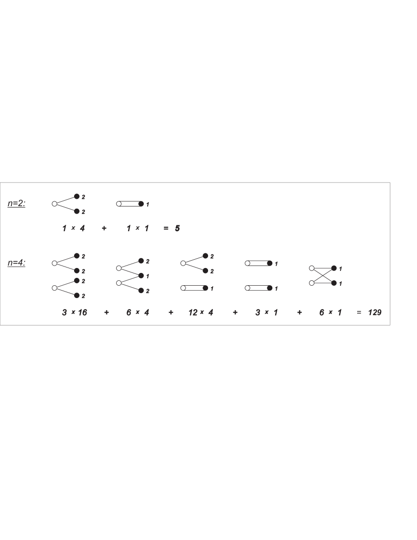
Figure 3: Lowest order Feynman-type graphs for Example 5 with $n=2,4$ lines. The number below each graph is $(multiplicity)\times\prod_{k}(vertex\ factor\ V_{k}=2\delta_{k,1}+\delta_{k,2})$.

In conclusion we see that the technique described herein and hinging on Eq.(9) leads to a combinatorial and graphical description of many physical systems.

References

References

[1] J.D.Bjorken and S.D.Drell, Relativistic Quantum Fields, (McGraw and Hill, St. Louis, 1965).
[2] A.N.Vasiliev, Functional Methods in
Quantum Field Theory and Statistical Physics, (Gordon and Breach, Amsterdam, 1998).
[3] J.R.Klauder and E.C.G.Sudarshan, Fundamentals
of Quantum Optics, (Benjamin, New York, 1968).
[4] W.H.Louisell, Quantum Statistical Properties of
Radiation, (J.Wiley, New York, 1990).
[5] W.M.Zhang, D.F.Feng and R.Gilmore, Rev. Mod. Phys.62, 867 (1990).
[6] R.M.Wilcox, J.Math. Phys.8, 962 (1967).
[7] P.Blasiak, K.A.Penson and A.I.Solomon,
Phys. Lett. A309, 198 (2003).
[8] M.A.Méndez, P.Blasiak, K.A.Penson and A.I.Solomon, (unpublished).
[9] C.M.Bender, D.C.Brody and B.K.Meister, J.Math. Phys.40, 3239 (1999);
C.M.Bender, D.C.Brody and B.K.Meister, Twistor Newsletter45, 36 (2000).