Vibrational coherent quantum computation

Abstract

A long-lived coherent state and non-linear interaction have been experimentally demonstrated for the vibrational mode of a trapped ion. We propose an implementation of quantum computation using coherent states of the vibrational modes of trapped ions. Differently from earlier experiments, we consider a far-off resonance for the interaction between external fields and the ion in a bidimensional trap. By appropriate choices of the detunings between the external fields, the adiabatic elimination of the ionic excited level from the Hamiltonian of the system allows for beam splitting between orthogonal vibrational modes, production of coherent states and non-linear interactions of various kinds. In particular, this model enables the generation of the four coherent Bell states. Furthermore, all the necessary operations for quantum computation such as preparation of qubits, one-qubit and controlled two-qubit operations, are possible. The detection of the state of a vibrational mode in a Bell state is made possible by the combination of resonant and off-resonant interactions between the ion and some external fields. We show that our read-out scheme provides highly efficient discrimination between all the four Bell states. We extend this to a quantum register composed of many individually trapped ions. In this case, operations on two remote qubits are possible through a cavity mode. We emphasize that our remote-qubit operation scheme does not require a high quality factor resonator: the cavity field acts as a catalyst for the gate operation.

I Introduction

Outstanding theoretical and experimental advances have been reported in the field of photonic quantum information processing, ranging from the experimental realization of the quantum teleportation protocol furusawa to proposals for quantum error correction ralph1 and quantum computation klm . It has been shown that universal continuous-variable quantum computation can be performed using linear optics (including squeezing), homodyne detection and non-linearities realized by photon-counting positive-valued-measurement bartlettsanders . Recently, a method to implement efficient universal computation based on coherent states of light has been suggested and shown to be robust against detection inefficiencies jacobmyung .

As pointed out in the Los Alamos Roadmap for quantum computing roadmap , using coherent states of a boson as logical qubits is one of the promising ways to realize quantum computation. However, one of the practical difficulties encountered in a scheme for coherent quantum computation is the requirement of a strong Kerr non-linear interaction to produce a superposition of coherent states. Currently available non-linear dielectrics, unfortunately, offer too low rates of non-linearity with exceedingly high absorption of the incoming field. In this context, some recent proposals for giant Kerr non-linear interaction exploiting electromagnetic induced transparency remains to be proved to work in the quantum domain ioEIT .

In this paper, we propose to implement coherent quantum computation using vibrational modes of trapped ions. Since the early days of the quantum manipulation of vibrational modes for trapped ions, it has been clear that strong non-linear evolutions can be efficiently engineered using two or three-level ions (in a $\Lambda$ configuration) interacting with properly tuned laser pulses wineland ; sasura ; STK ; lieb . Furthermore, a long-lived coherent state has been experimentally reported wineland ; lieb . This opens a way to the exploitation of vibrational states as the elements of a quantum register in a quantum processor. For the purposes of scalability, arbitrarily large quantum registers have to be considered. One way is to work with a chain of ions in the same trap, exploiting not just the vibrational modes of the centre of mass (CM) but the collective vibrational excitations of the chain (see wineland ; sasura and references within). Another way to realize the scalability is to take advantage of the recently demonstrated coupling between cavities and single-ion traps schmidt-kaler ; walther , which is the scheme used in this proposal. In our architecture, an array of many individually trapped ions constitute the quantum register. The local processors are interconnected via an effective all-optical bus realized by a cavity mode coupled to the different traps. We will not require a perfect cavity for our protocol and the cavity field mode never becomes entangled with the ions of the register (the coupling between two different ions being realized via a second-order interaction only virtually mediated by the cavity field).

In this paper, we also propose an efficient discrimination of the four quasi-Bell states embodied by entangled coherent states jacobmyung . In this respect, our detection scheme does not require the complete map of a quasi-Bell state onto the discrete electronic Hilbert space of the trapped ions munrosanders . The detection is performed exploiting the additional degree of freedom of the vibrational states represented by their even- and odd-number parities. It is worth stressing that the Bell-state discrimination can be accomplished, in our set-up, both locally (exploiting two orthogonal vibrational modes of a single trapped ion) and remotely, where the Bell state is the joint state of two vibrational modes of a linear two-ion crystal.

The paper is organized as follows. In Section II we describe the coupling scheme used in our proposal and address the issue of the preparation and single-qubit manipulation of coherent states. In this context, the generation of even/odd coherent states and entangled coherent state is discussed. We perform some quantitative investigations to prove that this coupling scheme allows for highly efficient quantum state engineering. In Section III, we propose the architecture for a distributed quantum register of many individually trapped ions interconnected by a cavity field mode. This proposal allows for vibrational quantum state transfer between two remote ions. We quantitatively address a non-trivial example. Section IV is devoted to the description of a scheme for almost complete Bell-state measurements performed combining vibrational-mode manipulations and electronic-state detection. The ability to achieve a high-efficiency discrimination of the four coherent Bell states is exploited. In Section V, we describe how to realize an entangling two-qubit gate that, together with the single-qubit rotations, allow for universal coherent quantum computation.

II Hamiltonian for quantum state engineering

The system we consider is a two-level ion coupled to a bichromatic field, detuned from the atomic transition. The trap tightly confines the ion in the $x-y$ plane (as sketched in Fig. 1 (a)). The energy scheme is shown in Fig.1 (b). The external fields (treated classically) illuminate the ion in opposite directions in the $z=0$ plane and both can have a component along the $x$ and $y$ axes. We assume the trap to be anisotropic, with $\omega_{x}>\omega_{y}$ and $\Delta{x}_{cm}$ ($\Delta{y}_{cm}$) the ground-state width, in the trapping potential, along the $x$ ($y$) direction. The Hamiltonian of the system reads ($\hbar=1$ is taken throughout this paper)

$$H=\sum_{i=x,y}\omega_{i}\hat{b}^{\dagger}_{i}\hat{b}_{i}+\omega_{eg}\hat{\sigma}_{+}\hat{\sigma}_{-}+\sum^{2}_{i=1}\left(\hat{g}_{i}\hat{\sigma}_{+}+\hat{g}^{\dagger}_{i}\hat{\sigma}_{-}\right).$$ (1)

Here, $\hat{b}^{{\dagger}}_{j}$ $(\hat{b}_{j})$ $(j=x,y)$ are the creation (annihilation) operators describing the quantized position of the CM of the ion in the trap, $\hat{g}_{i}=g_{i}{e}^{-i{\bf k}_{i}\cdot{\hat{\bf{r}}}-i\omega_{i}t-i\phi_{i}}$ take account of the couplings between the ion and the i-th laser ($i=1,2$) of its frequency $\omega_{i}$, wave-vector ${\bf{k}}_{i}\equiv(k_{ix},k_{iy},0)$ and phase $\phi_{i}$. Here, $\hat{\bf r}$ is the vectorial operator of the CM position and $\hat{\sigma}_{+}=\hat{\sigma}^{\dagger}_{-}=\left|e\rangle\langle g\right|$. The ion’s transition frequency is labelled by $\omega_{eg}$. In a rotating frame and in the limit of large detuning $\Delta_{1}\gg{g}_{1,2},\delta_{12},\gamma_{rad}$, where $\Delta_{1}=\omega_{eg}-\omega_{1}$, $\delta_{12}=\omega_{2}-\omega_{1}$ and $\gamma_{rad}$ the spontaneous decay-rate of the ion from $\left|e\right\rangle$, the atomic excited state can be adiabatically eliminated.

(a)                                   (b)

                 

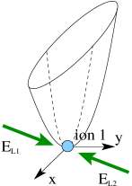
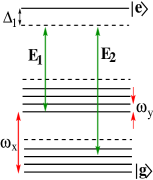
Figure 1: (a): The physical set-up. A two-level ion is trapped in a bidimensional trap ($\omega_{y}<\omega_{x}$). Two monochromatic laser field (classical) excite the ion. (b): The energy level scheme. The trap is quasi-harmonic so that, in the limit of resolved sidebands, the different excitations of the $x$ and $y$ vibrational degrees of freedom are spaced as shown. The lasers are off-resonance.

After some lengthy calculations and using the Campbell-Baker-Haussdorff theorem, the Hamiltonian can be written as

$$\begin{split}H&\simeq\sum_{j=x,y}\omega_{j}\hat{b}^{{\dagger}}_{j}\hat{b}_{j}-\frac{g_{1}g_{2}}{\Delta_{1}}\sum^{\infty}_{n,m=0}\sum^{\infty}_{p,q=0}\frac{(i{\eta}^{\prime}_{x})^{n+m}}{n!m!}\\ &\times\frac{(i\eta^{\prime}_{y})^{p+q}}{p!q!}\hat{b}^{{\dagger}{n}}_{x}\hat{b}^{m}_{x}\hat{b}^{{\dagger}{p}}_{y}\hat{b}^{q}_{y}e^{-i\delta_{12}t-i\phi}+h.c.\end{split}$$ (2)

where $\phi=\phi_{1}-\phi_{2}$ and a numerical factor arising from the normal ordering has been absorbed in the Rabi frequencies $g_{1,2}$. Here, $\eta^{\prime}_{x}=\Delta{x_{cm}}\Delta{k}_{x}$ and $\eta^{\prime}_{y}=\Delta{y_{cm}}\Delta{k}_{y}$ are the effective Lamb-Dicke parameters for the $x$ ($y$) motion respectively wineland and $\Delta{k}_{x,y}$ are the projections of ${\bf k}_{1}-{\bf k}_{2}$ in the $z=0$ plane. We have neglected the laser-intensity dependent ac-Stark shifts due to the dispersive couplings. These energy terms in the Hamiltonian can be controlled by stabilizing the laser beams and formally eliminated by redefining the ground state energy. A scheme to cancel the ac-Stark shifts using an additional laser has been demonstrated in ref. schmidtkalerstark . Properly directing the laser beams we can arrange a coupling between the two vibrational modes as well as engineering a single-mode Hamiltonian (when $\mu$ or $\nu$ is zero) STK . In this latter case, if not explicitly specified, we will always consider the states of the $x$ mode to embody the qubits, while the $y$ mode will be used as an ancilla. An interesting feature of the model in Eq. (2) is the possibility to select stationary terms from the Hamiltonian simply by tuning the laser fields to an appropriate sideband resonance of the trapped ion’s spectrum. Indeed, in the interaction picture, the term depending on $\exp\left[i(s_{x}\omega_{x}+s_{y}\omega_{y}-\delta_{12})t\right]$ (and its hermitian conjugate) appears in $H$, where $s_{x}=(n-m),\,s_{y}=(p-q)$. Tuning $\delta_{12}$, which excites the proper sideband of the energy-level scheme shown in Fig. 1 (b), we single out stationary terms in Eq. (2), which we want to be dominant over the contributions of the other oscillating terms.

A remarkable range of evolutions is covered by this coupling scheme and some of them are particularly relevant for the purpose of coherent quantum computation. We note that, in the protocol proposed in jacobmyung , the leading ingredients are represented by the ability to generate coherent states and their macroscopic superpositions (Schrödinger cat states) as well as multi-mode entangled coherent states. To manipulate the states of the elements of a quantum register, on the other hand, ref. jacobmyung prescribes the use of reliable beam splitter operations, phase shifts and displacement operations (these latter effectively perform rotations in the computational basis). A beam splitter (BS) operation has been described in ref. STK and we need to give details about the engineering of the other operations with our model.

We need a reliable way to generate a coherent state of motion in order to work in a computational space spanned by the coherent states $\left\{\left|\alpha\right\rangle,\left|-\alpha\right\rangle\right\}$ (which are quasi-orthogonal for sufficiently large $\alpha\in\mathbb{C}$). Many different ways to achieve this have been suggested wineland . Here, we note that, if $\delta_{12}=\omega_{x}$ (i.e. if we excite the first red sideband of the $x$ motion) and the two fields have no projection onto the $y$ axis, the stationary term $H_{cs}\simeq\left(i{g}_{1}g_{2}\eta^{\prime}_{x}/{\Delta_{1}}\right)\hat{b}^{{\dagger}}_{x}+h.c$ is selected, assuming $\phi=0$. This energy term gives rise to a unitary evolution that corresponds to a displacement $\hat{D}_{x}(\alpha)=\exp(\alpha\hat{b}_{x}^{\dagger}-\alpha^{*}\hat{b}_{x})$ in phase-space jacobmyung ; cochrane $\alpha=g_{1}g_{2}\eta^{\prime}_{x}t/\Delta_{1}$ and $t$ the interaction time. However, if we want to give an estimate of the accuracy of this state engineering procedure, the effect of the non-stationary terms in the Hamiltonian has to be quantitatively addressed. In order to do it, we consider the formal relationship between our coupling scheme and the system in ref. STK , where the three-level $\Lambda$ configuration can be mapped onto our own coupling-scheme when the adiabatic elimination of the excited state of the ion is performed. It is shown in STK that by considering an anisotropic trap with a sufficiently large ratio $\omega_{x}/\omega_{y}$, allows us to neglect additional accidental resonances in Eq. (2). To generate a coherent state, we estimate $\omega_{x}\geq 3\omega_{y}$ is enough. On the other hand, the coupling factors relative to the non-stationary terms in Eq. (2) are sensibly smaller than the rate at which the coherent state is generated once we guarantee $(g/\eta_{x}\Delta_{1})\ll\gamma$ with $\gamma=\omega_{x}/g$ a dimensionless parameter which, experimentally, can be $\gamma\geq{20}$. For the sake of definiteness, we have assumed $g_{1}=g_{2}=g$ and, given that $\delta_{12}\ll\omega_{1,2}$, we have taken $\left|k_{1}\right|\simeq\left|k_{2}\right|=k$ (so that $\eta^{\prime}_{x}\simeq{2\eta_{x}}$). For the realistic value $\eta_{x}=k\Delta{x}_{cm}=0.4$ , the above constraints require $\Delta_{1}\gg{g}/5$.

For our quantitative analysis, we choose $\omega_{x}=4\omega_{y}$ and $\Delta_{1}=5{g}$. Then, we retain the terms, in $H$, which oscillate at the frequencies $\omega_{x},\,\omega_{y},\,\omega_{x}{\pm}\omega_{y}$ so that the dynamic generator we consider is $H_{true}=H_{cs}+H_{nst}$, where $H_{nst}$ collects the non-stationary terms we discussed. With the above choices for the relevant parameters, we look for the overlap $\left|\left\langle\alpha|\psi\right\rangle_{t}\right|$ between the coherent state $\left|\alpha\right\rangle$ we want to generate and the state $\left|\psi\right\rangle_{t}=\exp\left\{-iH_{true}t\right\}\left|0\right\rangle_{x}$. Numerically, we are limited by the dimension of the computational space. We thus take $\left|\alpha\right|=1$ and truncate the basis to $\left\{\left|0\right\rangle,..,\left|5\right\rangle\right\}_{x}$, with $\left|n\right\rangle_{x}$ ($n=0,..,5$) indicating phonon-number states. On the other hand, the state of the $y$ mode should not be affected at all by the desired evolution. Assuming $\left|0\right\rangle_{y}$ for the initial state, it is reasonable to take $\left\{\left|0\right\rangle,\left|1\right\rangle\right\}_{y}$ for the evolution of this state due to $H_{true}$. The motional state of the ion at time $t$ is therefore expanded as $\left|\psi\right\rangle_{t}=\sum^{5}_{n,0}\sum^{1}_{m,0}A_{nm}(t)\left|n,m\right\rangle_{xy}$, with $\sum^{5}_{n,0}\sum^{1}_{m,0}\left|A_{nm}\right|^{2}=1$. The overlap reads ${\cal O}(t)={\cal N}\sum^{5}_{n=0}A_{n0}(t)/\sqrt{n!}$, (with ${\cal N}$ a normalization factor) that can be evaluated once we solve the set of differential equations obtained projecting the Schrödinger equation for $\left|\psi\right\rangle_{t}$ onto the $\left|n,m\right\rangle_{xy}$ states. The result is shown in Fig. 2 (a). The overlap becomes perfect when the rescaled interaction time is $gt=\Delta_{1}/(g\eta^{\prime}_{x})=6.25$. Furthermore, we have checked that with the above values the efficiency of the process is insensitive to an increase of the Lamb-Dicke parameter up to $\eta_{x}\simeq{0.9}$. For a larger $\eta_{x}$, some deviation from the ideal case is observed. Another parameter that is relevant in this investigation is $\gamma$. Reducing it means lowering the oscillation frequencies of the non-stationary terms in $H_{true}$. This spoils the efficiency of the entire state-engineering process. An example of this effect is given in Fig. 2 (b). It is worth stressing that, even though the generation of a coherent state with just a small amplitude $\alpha$ has been checked here, this will also apply for a larger (in principle arbitrary) amplitude.

(a)                                         (b)

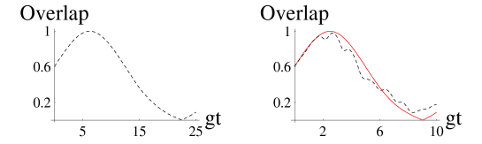
Figure 2: (a): The overlap between a coherent state $\left|\alpha=1\right\rangle_{x}$ and the state generated by the non-ideal Hamiltonian $H_{true}$ that contains non-stationary terms at low frequencies up to second order in the Lamb-Dicke parameter. In this simulation, $\eta_{x}=0.4$. Other parameters are as in the text. (b): Comparison between the perfect overlap (solid line) and the one obtained with $\eta_{x}=1.0$ and $\gamma=10$ (dashed line).

For a single qubit operation, we first consider the rotation $U^{z}(\theta/2)$ around the $z$ axis of the Bloch sphere for the qubit $\left\{\left|\pm\alpha\right\rangle\right\}_{x}$. This rotation is very well approximated by displacement operation $\hat{D}_{x}(i\epsilon)$, with $\epsilon=\theta/4\alpha$ $\left(\theta\in{[}0,2\pi]\right)$ jacobmyung .

$$U^{z}\left(\frac{\theta}{2}\right)=\begin{pmatrix}e^{i\frac{\theta}{2}}&0\\ 0&e^{-i\frac{\theta}{2}}\end{pmatrix}.$$ (3)

Indeed, $\hat{D}(i\epsilon)\left|\alpha\right\rangle_{x}=e^{2i\epsilon\alpha}e^{(\alpha+i\epsilon)\hat{b}^{{\dagger}}_{x}-(\alpha-i\epsilon)\hat{b}_{x}}\left|0\right\rangle_{x}=e^{2i\alpha\epsilon}\left|\alpha+i\epsilon\right\rangle_{x}\simeq{e}^{i\frac{\theta}{2}}\left|\alpha\right\rangle_{x}$, where the condition $\alpha\gg\epsilon$ has been assumed (keeping the product $\alpha\epsilon$ always finite). In practice, for $\alpha\gtrsim{2}$, a small $\epsilon$ is sufficient to perform a $2\pi$ rotation.

The rotation $\hat{U}^{x}(\pm\pi/4)$ jacobmyung around the $x$ axis of the qubit’s Bloch sphere can be performed by a Kerr interaction $H_{K}=\chi_{K}(\hat{b}^{{\dagger}}_{x}\hat{b}_{x})^{2}$. We now briefly describe the procedure to obtain such a Hamiltonian. Aligning the laser beams along the $x$ axis (to get $\mu=1,\,\nu=0$) and arranging their relative detuning $\delta_{12}=0$, we select a stationary term proportional to $\hat{b}^{\dagger{2}}_{x}\hat{b}^{2}_{x}$ in Eq. (2), with the corresponding rate of non-linearity $\chi_{K}=2g_{1}g_{2}\eta^{\prime 4}_{x}/\Delta_{1}$. We exploit the canonical commutation rules between $\hat{b}^{{\dagger}{}}_{x}$ and $\hat{b}_{x}$ and the relation $[\hat{n}_{x},\hat{n}^{2}_{x}]=0$ ($\hat{n}_{x}=\hat{b}^{{\dagger}}_{x}\hat{b}_{x}$), to obtain $\exp\left\{-iH_{K}{t}\right\}|_{\chi{t}=\pi/2}\left|\mp{i}\alpha\right\rangle_{x}=\frac{1}{\sqrt{2}}\left(\left|\alpha\right\rangle\pm{i}\left|-\alpha\right\rangle\right)_{x}$ yurkestoler . This macroscopic superposition of coherent states is the result of the rotation in the Bloch sphere $\{|\pm\alpha\rangle\}$.

In order to check the effects of the non-resonant terms in the Hamiltonian of our Kerr non-linear evolution, we have conducted an analysis similar to the one previously performed to generate a coherent state. This time, $H_{true}=H_{K}+H_{nst}$ contains terms oscillating at the lowest frequencies and up to the fourth power in $\eta_{x}$. The stationary term $H_{K}$ dominates over $H_{nst}$ because the effect of the high-frequency oscillating terms is averaged out from the effective dynamical evolution of the qubit. We retain the same values used before for the relevant parameters in our calculations, showing that they are suitable for this effective rotation too. Our model is sufficiently flexible not to require further adjustments of the set-up. We consider the transformation $\left|\alpha=-i\right\rangle_{x}\rightarrow\left|cat1\right\rangle_{x}=\frac{1}{\sqrt{2}}\left(\left|\alpha=1\right\rangle+i\left|\alpha=-1\right\rangle\right)_{x}$ and use the truncated phonon-number basis $\left\{\left|0\right\rangle,..,\left|5\right\rangle\right\}^{\otimes{2}}$ to solve the projected Schrödinger equations

$$i\,_{xy}\!\left\langle p,q\right|\partial_{t}\left|\psi(t)\right\rangle_{xy}=\,_{xy}\!\left\langle p,q\right|H_{true}\left|\psi(t)\right\rangle_{xy},$$ (4)

with $\left|\psi(0)\right\rangle_{xy}=\left|-i\right\rangle_{x}\left|0\right\rangle_{y}$ and the decomposition $\left|\psi(t)\right\rangle_{xy}=\sum^{5}_{n,m=0}A_{nm}(t)\left|nm\right\rangle_{xy}$. The normalization of the wave-function implies $\sum^{5}_{n,m=0}\left|A_{nm}(t)\right|^{2}=1$, as before.

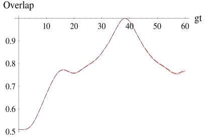
Figure 3: Comparison between the perfect overlap ${\cal O}_{id}(t)$ (broken line) and the true one ${\cal O}_{true}(t)$ obtained numerically solving the Schrödinger equation governed by $H_{true}$. In these calculations, $\eta_{x}=0.4$ and $g=500\pi\,KHz$. Other parameters are as described in the body of the paper.

In Fig. 3 we compare the ideal overlap ${\cal O}_{id}(t)=\left|{}_{x}\!\left\langle cat1|e^{-iH_{K}t}|-i\right\rangle_{x}\right|$ (dashed line) to the overlap ${\cal O}_{true}(t)=\left|{}_{xy}\!\left\langle cat1,0\right|{e^{-iH_{true}t}}\left|-i,0\right\rangle_{xy}\right|$ (solid curve), whose time behavior depends on the coefficients $A_{nm}(t)$, for counter-propagating lasers with $g_{1,2}=g$ and $\eta_{x}=0.4$. It is apparent that the dynamical evolution governed by $H_{true}$ leads to the desired superposition state at the expected rescaled time $gt=5\pi/2\eta^{\prime{4}}_{x}\simeq{38}$. The match between the two curves is very good up to the rescaled interaction times we show. Being a rotation in the space spanned by the coherent states with amplitude $\alpha=\pm{1}$, the behavior of the overlap is periodic and replicates itself for interaction times larger than those shown in Fig. 3. This numerical simulation suggests that Kerr non-linear interactions and, thus, the $U^{x}(\pm\pi/4)$ rotation, can actually be performed quite efficiently in this set-up. We estimate $\chi_{K}\simeq 20\pi\,KHz$, for $g=500\pi\,KHz$ wineland ; sasura , corresponding to an interaction time $t=\pi/2\chi_{K}\simeq 25\,\mu{sec}$. On the other hand, the effective life-time of the excited state $\left|e\right\rangle$, in the non-resonant regime we are considering, is $\tau_{spont}={\Delta^{2}_{1}}/({{g}^{2}}\gamma_{rad})\simeq{1}\,sec$ if we use metastable levels of an optical transition (for example the $S_{1/2}\rightarrow{D}_{5/2}$ transition in ${}^{40}Ca^{+}$ whose excited level has a natural life-time of about $1\,sec$ ($\gamma_{rad}\simeq{1\,sec}$) wineland ; schmidt-kaler ; schmidtkalerstark ).

We need here to make a remark: the analysis we have performed always assumes that the ancillary $y$ mode is prepared in the vacuum state. This is just for mathematical convenience. We have derived the equations of motion for the case of an initial coherent state $\left|\beta=1\right\rangle_{y}$ of the $y$-motional mode. Here, again, a small amplitude of the coherent state is taken because it is then possible to truncate the computational phonon-number basis, considerably simplifying the calculations. We have concluded that the comparison between $Ov_{id}(t)$ and $Ov_{true}(t)$ shows the same qualitative features seen in Fig. 3. We conjecture that the same conclusion holds regardless of the state in which the $y$ degree of motion has been prepared, if the parameter in $H_{true}$ are kept within the range of validity of the approximations above.

With arbitrary rotations around the $z$ axis (implemented via effective displacements) and $\pi/4$ rotations around the $x$ axis, it is actually possible to build up any desired rotation around the $y$ axis of the Bloch sphere. This, in turn, allows us to arbitrarily rotate the qubit around the $x$ axis jacobmyung . The two operations we have demonstrated are thus sufficient to realize any desired one-qubit rotation. In particular, the sequence $U^{z}(\pi/4)U^{x}(\pi/4)U^{z}(\pi/4)\left|\pm\alpha\right\rangle_{x}$ realizes the transformation $\left|\pm\alpha\right\rangle_{x}\!\rightarrow(1/\sqrt{2})\left(\left|\alpha\right\rangle_{x}\pm\left|-\alpha\right\rangle_{x}\right)$ that is a Hadamard gate. The resulting states, here, are the the so-called even (for $+$ sign) and odd (for $-$ sign) coherent states as they are the superposition of just even and odd phonon-number states, respectively ioEIT . An interesting feature that will be exploited later is that even and odd coherent states are eigenstates of the parity operator $(-1)^{\hat{n}}$ ($\hat{n}$ is the phonon-number operator) with eigenvalue $\pm{1}$, respectively. We will discuss later the role these states have in coherent quantum computation.

As a final relevant case treated here, we now consider the engineering of a bimodal non-linear interaction suitable for the generation of entangled coherent states (ECS) sanders . This class of states will be represented as

$$\begin{split}\left|\phi_{\pm}\right\rangle=N^{\phi}_{\pm}\left\{\left|\alpha,\alpha\right\rangle\pm\left|-\alpha,-\alpha\right\rangle\right\},\\ \left|\psi_{\pm}\right\rangle=N^{\psi}_{\pm}\left\{\left|\alpha,-\alpha\right\rangle\pm\left|-\alpha,\alpha\right\rangle\right\}.\\ \end{split}$$ (5)

States $\left|\phi_{\pm}\right\rangle$ and $\left|\psi_{\pm}\right\rangle$ can be generated by superimposing, at a $50:50$ BS, a zero-phonon state $\left|0\right\rangle$ with an even and odd coherent state, respectively. As an example, suppose that, via the procedure described above, we have created an even coherent state of the $x$ motional mode while $y$ is in its vacuum state. Arranging a BS interaction between $x$ and $y$ phonon modes STK , the joint state of the two vibrational modes is then transformed into one of the entangled coherent states above. Alternatively, $\left|\phi_{\pm}\right\rangle$ and $\left|\psi_{\pm}\right\rangle$ can be produced using the cross-phase modulation Hamiltonian $H_{cp}=\chi_{cp}\hat{n}_{x}\hat{n}_{y}$, with $\chi_{cp}$ the rate of non-linearity ioEIT . Starting from $\left|\alpha\right\rangle_{x}\left|\beta\right\rangle_{y}$, this interaction produces $\left|ecs\right\rangle_{xy}\propto\left|\alpha\right\rangle_{x}\left(\left|\beta\right\rangle+\left|-\beta\right\rangle\right)_{y}+\left|-\alpha\right\rangle_{x}\left(\left|\beta\right\rangle-\left|-\beta\right\rangle\right)_{y}$ when $\chi_{cp}t=\pi$ ioEIT , which can be reduced to the form of ECS in Eq. (5) through single-qubit manipulation. Thus, having already discussed how to perform one-qubit operations, we concentrate here on the generation of this kind of generalized ECS.

By inspection of $H_{cp}$, we recognize the necessity of an interaction symmetry in the two vibrational modes. This can be obtained directing the lasers at $45$ and $225$ degrees with respect to the $x$ axis. In this case, $\delta_{12}=0$ has to be set in order to select the stationary term $\chi_{cp}\hat{b}^{{\dagger}}_{x}\hat{b}_{x}\hat{b}^{{\dagger}}_{y}\hat{b}_{y}$ in Eq. (2) with $\chi_{cp}=2g_{1}g_{2}\eta^{\prime 2}_{x}\eta^{\prime 2}_{y}/\Delta_{1}$. The other terms in the Hamiltonian are rapidly oscillating and negligible if the same dynamical conditions we commented above are assumed. We consider ${\cal O}_{ecs}(t)=\left|{}_{xy}\!\left\langle ecs_{id}\right|{e^{-iH_{true}t}}\left|\alpha=1,\beta=1\right\rangle_{xy}\right|$, with $H_{true}=H_{cp}+H_{nst}$ the Hamiltonian containing both the desired non-linear interaction $H_{cp}$ and all the relevant non stationary terms. We have taken $\left|ecs_{id}\right\rangle_{xy}\!\propto\!\left|1\right\rangle_{x}\left(\left|1\right\rangle+\left|-1\right\rangle\right)_{y}+\left|-1\right\rangle_{x}\left(\left|1\right\rangle-\left|-1\right\rangle\right)_{y}$, where all the states appearing in this expression are coherent states of their amplitude $\left|\alpha\right|=\left|\beta\right|=1$. To evaluate ${\cal O}_{ecs}(t)$, the computational basis has been truncated to $\left\{\left|0\right\rangle,..,\left|5\right\rangle\right\}^{\otimes{2}}$, as usual. The results are shown in Fig. 4. The dashed line represents the ideal behavior of the overlap, that is, its time dependency when just the ideal interaction $H_{cp}$ is considered. This curve is contrasted with the overlap obtained when the full Hamiltonian $H_{true}$ is taken. The mismatches between the curves are very small and the overall comparison is excellent. Here, $\eta_{x}=\eta_{y}=0.4$ and all the other relevant parameters are the same as in the previous simulations. The rescaled time $gt\simeq 77$, where the overlap is almost perfect, is equivalent to an effective interaction time of $t\simeq{50}\,\mu{sec}$, using the same parameters of the previous calculations. The scheme appears, thus, to be robust against the spoiling effects of the non-stationary terms and is efficient within the coherence times of the physical system we consider.

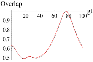
Figure 4: Comparison between the perfect overlap (dashed line) and the true one ${\cal O}_{ecs}(t)$ obtained solving the Schrödinger equation governed by $H_{true}$. In this simulation, $\eta_{x,y}=0.4$ and $g_{1,2}=g=500\pi\,{KHz}$. Other parameters as described in the body of the paper.

III Coupling between motional degrees of freedom of individually trapped ions

So far, our discussions have been limited to the case of a single ion. Unfortunately, considering the vibrational modes of just a single trapped ion is a substantial limitation on the computational capabilities of our device. However, we can take an advantage of some recent experiments that demonstrate the coupling between trapped ions and a high-finesse optical cavity walther ; schmidt-kaler to design the register of a vibrational quantum computer as formed by several remote and independently trapped ions. Here, we describe in detail a mechanism to couple the motional degrees of freedom of different elements of such a quantum register. In the experiments reported in refs. walther ; schmidt-kaler , a coherent interaction is established between an ion and a cavity mode. The optical transition between metastable states of a ${Ca}^{+}$ ion has been used to embody a qubit and the atomic responses to both temporal and spatial variations of the coupling have been analyzed schmidt-kaler . These impressive experimental achievements justify and motivate a posteriori the two-level model in the optical range of frequency we have assumed here. The system sketched in Fig. 5, is based on the linear geometry of the ion trap-optical cavity interfaces demonstrated in walther ; schmidt-kaler . This set-up is suitable to store a linear ion crystal represented by a row of aligned traps, which are mutually independent and spatially well-separated. The cavity field mode (here assumed to be a transverse $\mbox{TEM}_{00}$ mode of a near-confocal resonator) is described by its bosonic annihilation (creation) operator $\hat{a}$ ($\hat{a}^{{\dagger}}$) and is aligned with the $x$-axis of the bidimensional traps. The interaction with each ionic transition is off-resonant with detuning $\Delta_{i}$ ($i=1,2$) respectively (assumed to be different for sake of generality. The mathematical approach is simplified if $\Delta_{1}=\Delta_{2}$). Two external fields, $E_{L1},\,E_{L2}$ excite the ions and are directed along the $y$-axis. As we will see, this effectively couples the $y$ modes of the ions.

We assume a standing-wave configuration for the spatial distribution of the cavity field with the ions placed at the nodes of a cosine function commento ; sasura . In a rotating frame at the frequency $\omega_{L1}$ of the laser $E_{L1}$ and in the interaction picture with respect to the free energy of the resonator, the Hamiltonian of our system reads

$$\begin{split}H_{ic}=&\sum_{j=x,y}\sum^{2}_{i=1}\omega_{ji}\hat{b}^{{\dagger}}_{ji}\hat{b}_{ji}-\frac{{g}_{0}{\cal E}_{L1}\eta_{y1}}{\Delta_{1}}\left(\hat{b}^{{\dagger}}_{y1}+\hat{b}_{y1}\right)\hat{a}^{{\dagger}}e^{i\delta_{c}t}\\ &-\frac{{g}_{0}{\cal E}_{L2}\eta_{y2}}{\Delta_{2}}\left(\hat{b}^{{\dagger}}_{y2}+\hat{b}_{y2}\right)\hat{a}^{{\dagger}}e^{i(\delta_{c}+\Delta_{12})t+i\phi}+h.c.\end{split}$$ (6)

Here, $\delta_{c}=\omega_{cavity}-\omega_{L1}$ and $\Delta_{12}=\omega_{L1}-\omega_{L2}$ while ${\cal E}_{Li}\,(i=1,2)$ is the Rabi frequency of the interaction between ion $i$ and laser $E_{Li}$ and $\phi$ is the phase-difference between the lasers. The condition $\Delta_{1,2}>{\cal E}_{L1},{\cal E}_{L2},g_{0}$ underlies Eqs. (6), where the electronic excited states of the ions have been adiabatically eliminated. An intuitive picture of the dynamics of the system in this set-up is gained in the overdamped-cavity regime (or bad cavity limit), where the cavity decay-rate $\kappa$ is much larger than any other rate involved in Eq. (6).

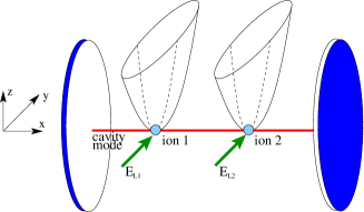
Figure 5: The set-up for a motional state transfer procedure. Two trapped ions are placed along the $x$ axis of a mono-mode optical cavity having a standing-wave configuration. The ions are coupled to the cavity field mode and to two external laser pulses. The laser fields illuminate the ions along the $y$ direction. This realizes an effective coupling between the $y$ vibrational modes of the trapped ions.

In this case, the cavity mode, which is detuned from the ionic transitions, represents an off-resonant bus that is only virtually excited by the interactions with the ions and can be eliminated from the dynamic of the overall system. In a formal way, we can consider the evolution equation of the cavity field operator $\hat{a}^{{\dagger}}$ and impose that its variations are negligible within the time-scale set by the effective coupling $\Omega_{i}=g_{0}{\cal E}_{Li}\eta_{yi}/\Delta_{i}$ ( that implies the cavity field mode has already reached its stationary state). This results in an effective interaction that, in a rotating frame at the frequencies of the traps (supposed to be identical for ion 1 and 2), reads

$$H^{rwa}_{ic}\simeq-\sum^{2}_{i\neq{j},1}\frac{{g}^{2}_{0}{\cal E}_{Li}{\cal E}_{Lj}\eta_{yi}\eta_{yj}}{\Delta_{i}\Delta_{j}\kappa}\left(\hat{b}^{{\dagger}}_{yi}\hat{b}_{yj}e^{i\phi}+\hat{b}^{{\dagger}}_{yj}\hat{b}_{yi}e^{-i\phi}\right),$$ (7)

where the condition $\Delta_{12}=\omega_{y2}-\omega_{y1}$ and the Rotating Wave Approximation (RWA) have been used. This interaction models a BS operation between motional degrees of freedom belonging to spatially separated trapped ions. This interaction is useful for entanglement generation and motional state transfer, where the states $\left|\psi\right\rangle_{y1}$ and $\left|0\right\rangle_{y2}$ are swapped, with $\left|\psi\right\rangle_{y1}$ being completely arbitrary. This is exactly what we want to realize for the purpose of motional state transfer. If the ion crystal is larger than two units, two specific ions can be connected by exciting them (and only them) with the laser fields. The other trapped ions will be unaffected by the coupling. Once the local interaction between the $x$ and $y$ motional modes of a specific ion has been performed (according to a given quantum computing protocol), then the state of the $y$ mode can be properly transferred to another ion of the crystal, labelled $l$, that has been prepared in $\left|0\right\rangle_{yl}$. However, for the sake of realism, in what follows we pursue the analysis restricted to a two-ion system and give some more insight in the process of motional state transfer.

The assumed bad cavity limit is particularly convenient to isolate the dynamics of the motional modes from that of the bus. Indeed, a full picture of the evolution of the system is gained by the master equation (in the interaction picture)

$$\partial_{t}\rho=-i\left[H^{\prime}_{ic},\rho\right]+\kappa\left(2\hat{a}\rho\hat{a}^{{\dagger}}-\left\{\hat{a}^{{\dagger}}\hat{a},\rho\right\}\right)=(\hat{\cal L}_{0}+\hat{\cal L}_{cav})\rho,$$ (8)

with $\rho$ the total density matrix of the $ion\,1+ion\,2+cavity$ system and, taking $\delta_{c}=\omega_{y1},\,\Delta_{12}=\omega_{y2}-\omega_{y1}$, it is $H^{\prime}_{ic}=-\sum^{2}_{i=1}\Omega_{i}(\hat{b}_{yi}\hat{a}^{{\dagger}}+h.c.)$. We have used the notation $\hat{\cal L}_{0}\rho=-i[H^{\prime}_{ic},\rho]$. We now go to a dissipative picture defined by $\tilde{\rho}=e^{-\hat{\cal L}_{cav}t}\rho$ and exploit the relations $\hat{\cal L}_{cav}[\hat{a},\rho]=[\hat{a},(\hat{\cal L}_{cav}-\kappa)\rho]$, $\hat{\cal L}_{cav}(\hat{a}\rho)=\hat{a}\hat{\cal L}_{cav}\rho+\kappa\hat{a}\rho$ (and analogous for $\hat{a}^{{\dagger}}$) iotransfer . After some lengthy calculations, Eq. (8) reduces to

$$\begin{split}\partial_{t}\tilde{\rho}&=i{g}_{0}\sum^{2}_{i=1}\frac{{\cal E}_{Li}\eta_{yi}}{\Delta_{i}}\left\{e^{-\kappa{t}}[\hat{b}_{yi},\tilde{\rho}]\hat{a}^{{\dagger}}+e^{\kappa{t}}\hat{b}_{yi}[\hat{a}^{{\dagger}},\tilde{\rho}]-h.c.\right\}\\ &\equiv{e}^{-\kappa{t}}\hat{\cal L}_{1}\tilde{\rho}+e^{\kappa{t}}\hat{\cal L}_{2}\tilde{\rho},\end{split}$$ (9)

with $\hat{\cal L}_{1}$ ($\hat{\cal L}_{2}$) an effective super-operator obtained by collecting all the terms in Eq. (9) having the $e^{-\kappa{t}}$ ($e^{\kappa{t}}$) pre-factor. To isolate the vibrational degrees of freedom, we trace over the cavity mode. We obtain $\partial_{t}\rho_{v}=\hat{\cal L}_{1}(e^{-\kappa{t}}\tilde{\rho})$, with $\rho_{v}=Tr_{cav}(\tilde{\rho})$. This master equation still involves the cavity variables because of the presence of $\tilde{\rho}$. In order to remove these dependencies, we go back to Eq. (8), integrate it formally and multiply it by $e^{-\kappa{t}}$. In the limit of large $\kappa$, we can invoke the first Born-Markov approximation and set $\tilde{\rho}=\rho_{v}\otimes\rho_{cav,ss}$ with $\rho_{cav,ss}$ the steady state of the cavity mode. It is, then, $e^{-\kappa{t}}\tilde{\rho}(t)\simeq\int^{\infty}_{0}\hat{\cal L}_{2}(\rho_{v}(t)\otimes\rho_{cav,ss})e^{-\kappa{t^{\prime}}}dt^{\prime}$ and

$$\begin{split}&\partial_{t}\rho_{v}=Tr_{cav}\left\{\hat{\cal L}_{1}\left(\int^{\infty}_{0}\hat{\cal L}_{2}(\rho_{v}(t)\otimes\rho_{cav,ss})e^{-\kappa{t^{\prime}}}dt^{\prime}\right)\right\}\\ &=\sum^{2}_{i,j=1}\frac{g^{2}_{0}{\cal E}_{Li}{\cal E}_{Lj}\eta_{yi}\eta_{yj}}{\Delta_{i}\Delta_{j}\kappa}\left\{\left[\hat{b}_{yi},\rho_{v}\hat{b}^{{\dagger}}_{yj}\right]-\left[\hat{b}^{{\dagger}}_{yi},\hat{b}_{yj}\rho_{v}\right]\right\}\\ &\equiv\sum^{2}_{i=1}\Gamma_{i}\left\{2\hat{b}_{yi}\rho_{v}\hat{b}^{{\dagger}}_{yi}-\rho_{v}\hat{b}^{{\dagger}}_{yi}\hat{b}_{yi}-\hat{b}^{{\dagger}}_{yi}\hat{b}_{yi}\rho_{v}\right\}+\\ &\sqrt{\Gamma_{1}\Gamma_{2}}\left[2\hat{b}_{y1}\rho_{v}\hat{b}^{{\dagger}}_{y2}+2\hat{b}_{y2}\rho_{v}\hat{b}^{{\dagger}}_{y1}-\left\{\hat{b}^{{\dagger}}_{y1}\hat{b}_{y2}+\hat{b}^{{\dagger}}_{y2}\hat{b}_{y1},\rho_{v}\right\}\right]\end{split}$$ (10)

with $\Gamma_{i}=\Omega^{2}_{i}/\kappa$ ($i=1,2$). This is the reduced master equation in our study. So far, we have not included the relaxation terms due to the decay of the motional amplitude of the ion modes. However, these can be included in the above derivation simply adding to Eq. (8) the Liouvillian terms proportional to the vibrational decay-rate $\gamma_{v}$ (assumed to be equal for the $x$ and $y$ motion). These terms do not depend on the cavity operators and are left unaffected by the adiabatic elimination of the field mode. Their inclusion will eventually result in a modification of just the single mode effective rates according to $\Gamma_{i}\rightarrow\Gamma_{i}+\gamma_{v}$. Of course, there is still much more to understand about the mechanisms that lead to vibrational decoherence murao . However, some estimates of $\gamma_{v}$ put it in the range of tens of milliseconds (see wineland and Roos et al. in murao ) and, as we will see, we estimate them to be longer than the effective interaction times required for a complete motional state transfer. Thus, from now on, we drop $\gamma_{v}$ from our analysis. Eq. (10) can be projected onto the phonon-number basis $\left\{\left|n,m\right\rangle\right\}_{y1,y2}$ to give effective evolution equations that are used for a numerical estimation of the dynamics of ${\rho}_{v}$.

As an example of motional state transfer, we quantitatively address the case of $\left|\psi\right\rangle_{y1}=\sqrt{2/5}\left(\left|0\right\rangle-\left|1\right\rangle\right)_{y1}+\sqrt{1/5}\left|2\right\rangle_{y1}$, where $(|0\rangle,~{}|1\rangle,~{}|2\rangle)_{y1}$ are phonon-number states, being prepared in ion $1$. Here, the choice has been completely arbitrary (any other state could have been taken). However, this example offers us the possibility to see the influence of our protocol on relative phases in general linear superpositions. Furthermore, the possible leakage into the Hilbert space complementary to the one spanned by our computational basis can be investigated. For quantitative calculations, we restrict the basis to $\left\{\left|0\right\rangle,..,\left|3\right\rangle\right\}^{\otimes{2}}$. For the transfer protocol to be effective, the state of the $y2$ mode must be prepared in $\left|0\right\rangle_{y2}$. Some comments are necessary in order to clarify the protocol. From now on, we refer to the ion whose $y$ motional state has to be transferred as the transmitter while the receiver is the ion prepared in $\left|0\right\rangle_{y}$. The interaction channel between the transmitter and the receiver is open if and only if both the ions are illuminated by the external laser fields. This means that, once one of the lasers is turned off, the transfer process stops and the interaction channel is interrupted and unable to further affect the joint state of the two ions. On the other hand, the effective interaction has to last for a time sufficient to complete the transfer. We find that temporally counter-intuitive laser pulses have to be applied to the system of transmitter-receiving ions. In particular, an efficient motional state transfer is achieved if the effective coupling rate $\Omega_{2}$ decreases while $\Omega_{1}$ increases in such a way that $\int_{\mathbf{T}}{dt^{\prime}}\sqrt{\Gamma_{1}(t^{\prime})\Gamma_{2}(t^{\prime})}=\vartheta=\pi/2$, where $\mathbf{T}$ is the total interaction period and time-dependent laser pulses have been assumed. An example of such pulses is given by $\Gamma_{1}(t)=\Gamma_{2}(-t)=\tilde{\Gamma}{e^{-\tilde{\Gamma}{t}}}/\left({e^{\tilde{\Gamma}{t}}+e^{-\tilde{\Gamma}{t}}}\right)$ mabuchi . We have assumed ${\cal E}_{L1}={\cal E}_{L2}={\cal E}_{L}$, $\eta_{y1}=\eta_{y2}=\eta_{y}$ and $\Delta_{1}=\Delta_{2}=\Delta$, so that $\tilde{\Gamma}=2g^{2}_{0}{\cal E}^{2}_{L}\eta^{2}_{y}/\Delta^{2}\kappa$. The time behaviors of $\Gamma_{1},\,\Gamma_{2}$ and $\sqrt{\Gamma_{1}\Gamma_{2}}$ are shown in Fig. 6 (a). To satisfy the conditions for the adiabatic elimination of the cavity mode ($\Omega_{1},\,\Omega_{2}\ll{\kappa}$), we have taken $\tilde{\Gamma}=0.03$.

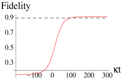
Figure 6: (a): We plot $\Gamma_{1}(t)$ (dashed line), $\Gamma_{2}(t)$ (dot-dashed) and $\sqrt{\Gamma_{1}(t)\Gamma_{2}(t)}$ (solid line) as a function of the rescaled interaction time $\kappa{t}$ and for $\tilde{\Gamma}=0.03$. The interaction channel is open at $t=-200\kappa^{-1}$. The fidelity does not reach $1$ because of the effective dissipative part in the evolution of the vibrational state that, actually, raises the vacuum component of the joint vibrational state. (b): Fidelity of motional state transfer $\left|\psi,0\right\rangle_{y1,y2}\rightarrow\left|0,\psi\right\rangle_{y1,y2}$ as a function of the interaction time $\kappa{t}$. After the interaction channel is closed, the state of the two vibrational modes is stationary.

The time integration of the effective coupling rate range where the amplitudes of the laser pulses are non-zero gives $\vartheta\simeq\pi/2$, so we expect that, after the effective interaction mediated by the cavity mode, the $y1$ motional state has been transferred to $y2$. This can be seen plotting the fidelity ${\cal F}_{\psi}(t)=_{y1,y2}\!\left\langle 0,\psi\right|{\$(\rho_{\psi})}\left|0,\psi\right\rangle_{y1,y2}$, as a function of $\kappa{t}$. Here, $\$$ is the map given by the reduced master equation we have derived. It takes the initial density matrix $\rho_{\psi}=\left|\psi,0\right\rangle_{y1,y2}\!\left\langle\psi,0\right|$ into $\rho_{v}(t)$, the solution of Eq. (10). The fidelity turns out to be a function of the interaction time and is parametrized by the state we want to transfer. The results of our simulation are presented in Fig. 6 (b). The fidelity is very good, reaching $\simeq 0.9$ for $t\gtrsim 200\kappa^{-1}$. We have plotted ${\cal F}_{\psi}(t)$ for interaction times larger than $\mathbf{T}$ to show that, once the effective coupling is turned off, the interaction channel breaks down and the state of the ions becomes stationary. It is worth stressing that the fidelity at the beginning of the interaction is non-zero because of the presence of $\left|00\right\rangle_{y1,y2}$ in both the initial and target states.

The second important point that has to be addressed in order to completely characterize the performance of the state transfer protocol is the leakage. We can single out two different kinds of leakage. One kind is to states such as $\left|i,j\right\rangle_{y1,y2}$ ($i,j\in\{1,3\}$) which are the states of the computational basis having more than $2$ phonons in the $y2$ mode and some phonons in the $y1$ mode. The other kind of leakage leads to states lying outside the computational space. The influence of both these sources of error can be contemplated looking at the norm of the final density matrix $\rho_{v}(t)=\$(\rho_{\psi})$. We have checked that $Tr(\rho_{v}(t))=1$ for all the relevant interaction times, showing that the influence of highly excited phononic states in the vibrational modes can be neglected. This indirectly demonstrates that leakage of the latter kind is irrelevant and the dynamics of the system is confined in the computational space we have chosen. On the other hand, by considering the quasi-norm ${\sum^{2}_{i=0}}\,_{y1,y2}\!\left\langle 0i\right|{\$(\rho_{\psi})}\left|0i\right\rangle_{y1,y2}$, we can check how large the influence of populated $y1$ states is in the density matrix $\rho_{v}(t)$. This is shown in Fig. 7 (a)

(a)                                           (b)

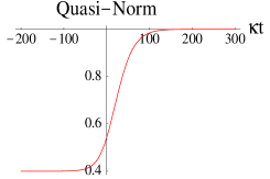
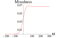
Figure 7: (a): The quasi-norm ${\sum^{2}_{i=0}}_{y1,y2}\!\left\langle 0i|\$(\rho_{\psi})|0i\right\rangle_{y1,y2}$ is plotted versus the interaction time $\kappa{t}$. This quantity considers the contribution to the normalization of the density matrix given by the states having just the $y2$ mode populated. (b): The degree of mixedness of $\rho_{v}(t)$ versus the interaction time $\kappa{t}$. The purity of the state is measured by the linearized entropy $S_{L}=(16/15)\left[1-Tr(\rho^{2}_{v})\right]$ that is zero for a perfectly pure state (as the initial one, at $\kappa{t}=-200$) and $1$ for a statistical mixture.

where we can see that, after the transient period when the contribution by non-empty states of the $y1$ mode is relevant, the steady state of the system is perfectly normalized. This means that the final state of the two vibrational modes does not contain excitations of the transmitter. To complete this analysis, we give some insight about the purity of the state we get. From this viewpoint, the fidelity is not a good tool because it could give the same quantitative results for $\rho_{v}(t)$ describing a pure state or a statistical mixture. On the other hand, an easily computable quantity is the linearized entropy $S_{L}(t)=(16/15)\left[1-Tr(\rho^{2}_{v}(t))\right]$  commento2 . This quantity is zero for a pure state and reaches $1$ if the state is completely mixed. We show a plot of $S_{L}(t)$ in Fig. 7 (b). The state remains highly pure all along the interaction, the small degree of mixedness being due to the dissipative nature of the effective evolution of the system arising from the bad-cavity regime.

The fidelity and purity of the state is not perfect because of the losses induced on the two-mode vibrational subsystem by the dissipative bus. However, the state we get with this protocol is nearly optimal. Higher quality factors of the optical cavity coupled to the ion traps will improve the performances. In this case, indeed, we would be able to neglect the dissipative dynamics of the cavity mode, making the effective interaction between transmitter and receiver perfectly unitary. The form of the effective Hamiltonian, arising from the coupling scheme, will be as in Eq. (7) with the replacement $\kappa\rightarrow\delta_{c}$ as, in this case, the condition $\delta_{c}\gg\kappa$ has to be used. The fidelity of the operation and the purity of the final state will be ideal. Unfortunately, this is not the case of the experiments performed in schmidt-kaler , where the cavity decay-rate is $\kappa\simeq{2\pi}\times 102\,KHz$ and has to be contrasted to the ion-cavity coupling $g_{0}\simeq 2\pi\times{134}Hz$. These cavity parameters, an external laser-ion Rabi frequency ${\cal E}_{L}\simeq{30}\,KHz$ with Lamb-Dicke parameter $\eta_{y}\simeq 0.2$ and detuning $\Delta\simeq{50}\,KHz$ (larger than a typical laser bandwidth $\sim 6{KHz}$) allow us to get an effective coupling rate $\tilde{\Gamma}\simeq 0.03$. This, in turn, gives interaction times in the range of $0.1\,msec$, smaller than the effective lifetime of the ion’s excited state. It is noticeable that we do not require a high-quality factor cavity to achieve an almost perfect motional state transfer, a feature of the protocol we have proposed that is certainly important from the practical viewpoint.

IV Quasi-Bell states measurement

We next consider the Bell-state measurement needed in the protocol for coherent quantum computation jacobmyung . As we will see in Section V, Bell-measurements can be used to construct the teleportation-based ${\sf CNOT}$ suggested by Gottesman and Chuang gottesman . In our specific case, the quantum channel for the teleportation protocol is embodied by one of the ECS’s in Eq. (5). For sufficiently large amplitudes of their components, the ECS are quasi-orthogonal, carry exactly one ebit of entanglement and are usually referred to as quasi-Bell states. A complete discrimination of the elements of this class is, thus, fundamental in our scheme. It is worth stressing here the well-known no-go theorem demonstrating that a never-failing, full Bell-state analyzer can not be realized using just linear interactions (e.g. beam splitters and phase shifters) norbert . More recently, it has been recognized that the introduction of a Kerr non-linear interaction vitalitombesi or the exploitation of additional degrees of freedom of the system employed beennaker can be used to fully discriminate all four Bell states. However, these schemes are designed to work with two-level systems and are not relevant to the infinite dimensional case we treat.

The direct detection of the properties of a vibrational state is, in general, a hard task to accomplish. On the other hand, detecting the electronic state of an ion (or an array of ions) is more straightforward and can be performed using the quantum jump technique, in which resonance fluorescence from a strongly driven atomic transition is detected wineland ; sasura ; lieb ; blattzoller . The presence/absence of fluorescence in the driven transition reveals the electronic state of the ion. Thus, we need a joint interaction that changes the internal degrees of freedom of the ion in a way that reflects the state of the vibrational ones. The measurement of the electronic state of the ion after the interaction, then, will give information on its vibrational state. To achieve this goal, we start by considering the Hamiltonian obtained by applying a standing-wave laser field to the trapped ion. In a rotating frame and with $\Delta=\omega_{eg}-\omega_{L}$ the detuning between the standing-wave and the ion’s transition frequency, the interaction reads

$$H^{\prime}={\Delta}\hat{\sigma}_{z}+{\omega_{x}}\hat{b}^{{\dagger}}_{x}\hat{b}_{x}+\Omega\cos[\eta(\hat{b}^{{\dagger}}_{x}+\hat{b}_{x})](\hat{\sigma}_{-}+\hat{\sigma}_{+}),$$ (11)

where $\Omega$ is the corresponding Rabi frequency. In the dispersive limit $\Delta\gg\Omega$, with $\Delta$ well-away from the resonant vibrational frequency (see Schneider and Milburn in murao ), we can adiabatically eliminate the excited state of the ion and expand $\cos[\eta(\hat{b}^{{\dagger}}_{x}+\hat{b}_{x})]$ in power series, retaining terms up to the second order in $\eta$ (Lamb-Dicke limit). In the interaction picture and neglecting terms oscillating at frequency $\pm{2}\omega_{x}$, we get

$$H_{qnd}\simeq{2}\frac{\Omega^{2}}{\Delta}\eta^{2}\hat{b}^{{\dagger}}_{x}\hat{b}_{x}\hat{\sigma}_{z},$$ (12)

where state-independent energy terms have been omitted. This Hamiltonian is suitable for quantum non-demolition measurements of the motional even/odd coherent states discussed above. Indeed, the evolution operator $\hat{U}_{qnd}(t)=\exp\left(-iH_{qnd}t\right)$ does not change the parity of an even/odd coherent state but phase-shifts the electronic state by an amount depending on the vibrational state phonon-number. Explicitly:

$$\begin{split}\hat{U}_{qnd}(t)&=\cos(\chi_{qnd}t\hat{b}^{{\dagger}}_{x}\hat{b}_{x})\mbox{$1{\bf l}$}-i\sin(\chi_{qnd}t\hat{b}^{{\dagger}}_{x}\hat{b}_{x})\hat{\sigma}_{z}\\ &=e^{i\chi_{qnd}t\hat{b}^{{\dagger}}_{x}\hat{b}_{x}}\left|g\rangle\langle g\right|+e^{-i\chi_{qnd}t\hat{b}^{{\dagger}}_{x}\hat{b}_{x}}\left|e\rangle\langle e\right|,\end{split}$$ (13)

with $\chi_{qnd}=2\Omega^{2}\eta^{2}/\Delta$. If we set $\chi_{qnd}t=\pi/2$, the electronic states will be mutually shifted $\pi$-out-of-phase.

Now, let us assume that we prepare the $x$ vibrational mode of an ion in an even/odd coherent state ${\cal N}_{\pm}(\left|\alpha\right\rangle\pm\left|-\alpha\right\rangle)$, while its internal state is $\left|g\right\rangle$. Then, we apply a $\pi/2$-pulse tuned on the carrier frequency of the ion’s spectrum. This particular interaction realizes the Hamiltonian $H_{car}={\cal G}\hat{\sigma}_{+}+h.c.$ that couples $\left|gn\right\rangle\leftrightarrow\left|en\right\rangle$ (${\cal G}$ being a Rabi frequency). That is, it does not affect the vibrational state wineland . The $\pi/2$-pulse prepares the superposition $(1/\sqrt{2})\left(\left|e\right\rangle+\left|g\right\rangle\right)$. The standing-wave described above is then applied and the interaction lasts for $t=\pi/2\chi_{qnd}$. This step of the protocol is used to write the vibrational state on the internal degrees of freedom of the ion. Another carrier-frequency $\pi/2$-pulse mixes up the phase-shifted components of the electronic state and, finally, the internal state detection is performed via quantum jumps. It is worth stressing that the electronic state detection is a true projective measurement (in the Von Neumann sense) that is able to tell us if the ion was in $\left|g\right\rangle$ or not. In this latter case, the vibrational state is reconstructed depending on the outcome of this last step. The described protocol realizes the transformations

$$\begin{split}{\cal N}_{+}\left(\left|\alpha\right\rangle+\left|-\alpha\right\rangle\right)\left|g\right\rangle\rightarrow\left(\left|i\alpha\right\rangle+\left|-i\alpha\right\rangle\right)\left|g\right\rangle,\\ {\cal N}_{-}\left(\left|\alpha\right\rangle-\left|-\alpha\right\rangle\right)\left|g\right\rangle\rightarrow\left(\left|i\alpha\right\rangle-\left|-i\alpha\right\rangle\right)\left|e\right\rangle.\end{split}$$ (14)

Thus, the different parity of the two vibrational states affects differently the interference between the components of the Fourier-transformed state $\left|g\right\rangle$. The discrimination between even and odd coherent states can be performed with, in principle, high accuracy. Each step in the protocol can be, indeed, quite precisely performed if a judicious choice of the parameters is made. The preparation of the electronic state superposition can be done off-line, exploiting one of the two laser beams that build up the standing-wave and reminding that the effective Hamiltonian in Eq. (2) does not affect the electronic variables of the ion (the manipulation of the electronic state then has no influence on the vibrational states). An estimate of the interaction time required to perform $\hat{U}(\pi/2\chi_{qnd})$ and to achieve the right phase shift leads to $\sim 15\,\mu{sec}$ for $\Omega=\pi\times{500}\,KHz$, $\eta=0.2$ and $\Delta=10\,MHz$ myungscheme .

This protocol, which was studied for the cavity quantum electrodynamic model to detect even and odd parities of the cavity field englert , is useful for the detection scheme for ECS. In particular, let us suppose an ECS state of the $x$ and $y$ modes of an ion is subject to a $50:50$ BS operation. This will give us one of the output modes in an even/odd coherent state, the other being in its vacuum. In particular

$$\begin{split}\hat{B}_{xy}\left(\frac{\pi}{4}\right)\left|\phi_{\pm}\right\rangle_{xy}&=N^{\phi}_{\pm}\left\{\left|\sqrt{2}\alpha\right\rangle\pm\left|-\sqrt{2}\alpha\right\rangle\right\}_{x}\otimes\left|0\right\rangle_{y},\\ \hat{B}_{xy}\left(\frac{\pi}{4}\right)\left|\psi_{\pm}\right\rangle_{xy}&=N^{\psi}_{\pm}\left|0\right\rangle_{x}\otimes\left\{\left|\sqrt{2}\alpha\right\rangle\pm\left|-\sqrt{2}\alpha\right\rangle\right\}_{y},\\ \end{split}$$ (15)

where $\hat{B}_{xy}(\pi/4)$ is the $50:50$ BS operator burnett . Then, the following protocol could be used. We prepare the electronic state of the trapped ion in the ground state and apply a carrier-frequency $\pi/2$-pulse to get the electronic superposition $\left(\left|e\right\rangle+\left|g\right\rangle\right)/\sqrt{2}$. Then, we arrange the evolution $\hat{U}_{qnd}(t/2\chi_{qnd})$ for the electronic+$x$-vibrational subsystem. Another carrier-frequency $\pi/2$-pulse on the ion mixes the components of the electronic superpositions. A quantum-jump detection reveals the internal state and the output is recorded. If the result of the measurement is $\left|g\right\rangle$, the entire protocol is re-applied, this time arranging the $\hat{U}_{qnd}(t/2\chi_{qnd})$ evolution of the electronic+$y$-vibrational subsystem. If the result of the first electronic detection is instead $\left|e\right\rangle$, we use a $\pi$-carrier pulse that restores $\left|g\right\rangle$, before the protocol is re-applied (this can be done with, in principle, $100\%$ of accuracy wineland ). The different combinations in which the internal state of the ion is found allows us for a partial discrimination between the elements in the ECS class. Denoting $|even,i\sqrt{2}\alpha\rangle_{j}$ and $|odd,i\sqrt{2}\alpha\rangle_{j}$ ($j=x,y$), respectively, the even and odd coherent states whose components have absolute amplitude $\left|i\sqrt{2}\alpha\right|$, one can prove the correspondences shown in Tab. 1.

Initial state	$1^{st}$ det.	$2^{nd}$ det.	Final vibrational state
$\left|\phi_{+},g\right\rangle_{xy,ion}$	$\left|g\right\rangle_{ion}$	$\left|g\right\rangle_{ion}$	$\left|even,i\sqrt{2}\alpha\right\rangle_{x}\otimes\left|0\right\rangle_{y}$
$\left|\phi_{-},g\right\rangle_{xy,ion}$	$\left|e\right\rangle_{ion}$	$\left|g\right\rangle_{ion}$	$\left|odd,i\sqrt{2}\alpha\right\rangle_{x}\otimes\left|0\right\rangle_{y}$
$\left|\psi_{+},g\right\rangle_{xy,ion}$	$\left|g\right\rangle_{ion}$	$\left|g\right\rangle_{ion}$	$\left|0\right\rangle_{x}\otimes\left|even,i\sqrt{2}\alpha\right\rangle_{y}$
$\left|\psi_{-},g\right\rangle_{xy,ion}$	$\left|g\right\rangle_{ion}$	$\left|e\right\rangle_{ion}$	$\left|0\right\rangle_{x}\otimes\left|odd,i\sqrt{2}\alpha\right\rangle_{y}$

Table 1: We schematically present the protocol for a partial quasi-Bell states discrimination. The initial state (the vibrational $x$ and $y$ modes being prepared in an ECS), the outcomes of the $1^{st}$ and $2^{nd}$ electronic measurement and the final vibrational state are displayed.

It is seen that, while the discrimination between $\left|\phi_{-}\right\rangle_{xy},\,\left|\psi_{-}\right\rangle_{xy}$ and $\left\{\left|\phi_{+}\right\rangle,\left|\psi_{+}\right\rangle\right\}_{xy}$ is perfect, this is not the case for the elements of the subset $\left\{\left|\phi_{+}\right\rangle,\left|\psi_{+}\right\rangle\right\}_{xy}$. The sequence of detected electronic measurements corresponding to these vibrational states is the same and there is no way to distinguish between them, following this strategy. However, one can exploit the parity non-demolition nature of the above procedure. Even if the amplitudes of the components of an even/odd coherent state are changed (the amplitude transforming from $\left|\alpha\right|$ to $\left|i\sqrt{2}\alpha\right|$), the parity eigenvalue of these states is preserved.

Now, if $\left|\phi_{+}\right\rangle_{xy}$ is prepared instead of $\left|\psi_{+}\right\rangle_{xy}$, we end up with mode $x$ being populated while $y$ is in its vibrational vacuum state. The configuration will be contrary if $\left|\psi_{+}\right\rangle_{xy}$ is prepared. Thus, the key of our procedure is the discrimination between $\left|0\right\rangle_{x}$ and $\left|even,i\sqrt{2}\alpha\right\rangle x$. Let us suppose that, after the application of the previous protocol and having found a sequence of two ground states as a result of the detection procedure (with the prepared vibrational state being totally unknown), we apply the displacement operator $\hat{D}(-\epsilon)$ to mode $x$, $\epsilon$ being a proper amplitude. If $\left|\phi_{+}\right\rangle_{xy}$ was the initial state, the displacement transforms the state of the $x$ mode into $\left(e^{i2\sqrt{2}\alpha\epsilon}\left|i\sqrt{2}\alpha-\epsilon\right\rangle+e^{-i2\sqrt{2}\alpha\epsilon}\left|-i\sqrt{2}\alpha-\epsilon\right\rangle\right)_{x}$. Taking $2\sqrt{2}\alpha\epsilon=\pi/2$ and $\alpha=2$, then we get $\epsilon\simeq{0.27}\ll\alpha$. With this angle of rotation the even coherent state is changed into an approximation of an odd one. We have flipped the parity of the state. Applying now the quasi-Bell state detection protocol, as described above, the outcome of the first atomic measurement becomes $\left|e\right\rangle_{ion}$. Does it help in distinguishing between $\left|\phi_{+}\right\rangle_{xy}$ and $\left|\psi_{+}\right\rangle_{x1x2}$? The effect of displacement on the state $\left|0\right\rangle_{x}\otimes\left(\left|i\sqrt{2}\alpha\right\rangle+\left|-i\sqrt{2}\alpha\right\rangle\right)_{y}$ (that is the final vibrational state if $\left|\psi_{+}\right\rangle_{xy}$ is prepared, as shown in Tab. 1) is $\left|0\right\rangle_{x}\rightarrow\left|-\epsilon\right\rangle_{x}$. For the amplitudes of the coherent state $\alpha$ and the angle of rotation $\epsilon$ chosen above, however, it is $\left|-\epsilon\right\rangle_{x}\simeq 0.96\left|0\right\rangle_{x}-0.27\left|1\right\rangle_{x}$. Applying again the ECS detection scheme, just before the first electronic detection, we get

$$\begin{split}&\left|-\epsilon\right\rangle_{x}\otimes\left|even,i\sqrt{2}\alpha\right\rangle_{y}\otimes\left|g\right\rangle_{ion}\\ &\rightarrow(0.96\left|0\right\rangle\left|g\right\rangle-i0.27\left|1\right\rangle\left|e\right\rangle)_{x,ion}\otimes\left|even,i\sqrt{2}\alpha\right\rangle_{y}.\end{split}$$ (16)

The probability to get the electronic output $\left|e\right\rangle_{ion}$ is given by $(0.27)^{2}\ll(0.96)^{2}$. That is, most of the times (approximately $92\%$ of the times) we will obtain $\left|g\right\rangle_{ion}$, making the discrimination between the two states complete. This can be taken as an estimate of the efficiency of the quasi-Bell state measurement because, in the present case, the efficiency of the detector apparatus (that is the efficiency of the quantum jumps technique for electronic state’s detection) can be taken, nominally, $100\%$ blattzoller . Our protocol for quasi-Bell state measurements can be adapted to the case of two distinct vibrational modes relative to remote trapped ions. It could be re-designed, mutatis mutandis, using two ions and their $x$ motional modes. In this case, the internal degrees of freedom have to be detected in parallel and not sequentially and the discrimination will be based on the comparison between different combinations of them. Considering all the operations to be performed before the ion’s internal-state detection, the overall time required for a complete discrimination of ECS should be in the range of hundreds of $\mu{sec}$, which is within the coherence times of the system.

V Controlled two-qubit gates

In this Section, we consider controlled two-qubit gates to complete our discussion on a possibility of qubit operations using coherent states of vibrational modes of ions. As we have remarked in the previous Section, a quasi-Bell state detection (both local and distributed) is possible. The teleportation-based scheme for a CNOT, indeed, exploits the Bell state measurements to perform two different steps. We follow the scheme proposed in jacobmyung and consider two three-mode GHZ states, $\left|\xi\right\rangle_{a0,a1,a2}$ and $\left|\xi\right\rangle_{a3,a4,a5}$, of general bosonic modes $a0,..,a5$. The joint state of modes $a0$ and $a3$ is first projected onto the Bell basis in order to prepare the (un-normalized) four-mode entangled state

$$\begin{split}\left|\eta\right\rangle_{anc}=\left|\alpha,\alpha\right\rangle_{a1,a2}\left|\phi_{+}\right\rangle_{a4,a5}+\left|-\alpha,-\alpha\right\rangle_{a1,a2}\left|\psi_{+}\right\rangle_{a4,a5}.\end{split}$$ (17)

This is then used to realize the ${\sf CNOT}$ gate as described in refs. jacobmyung ; gottesman . The GHZ states can be built by using beam splitters STK and single-mode rotations as those already demonstrated above. It has been recently recognized (see for example ralph ) that the four-mode state, being a complicated step to perform, can be prepared off-line and then used in the protocol for the CNOT only when it is needed. Overall, we need $8$ vibrational modes to implement a single CNOT, six of which are used to prepare for $\left|\eta\right\rangle_{anc}$ and the remaining two for the control and target qubits. In our scheme, however, we use two vibrational modes per ion so that we require $4$ ions and many motional state transfer operations. Even if there is no in-principle difficulty in doing this, it is apparent that the scheme is experimentally challenging, not just for the in situ operations to perform (linear and non-linear coupling between orthogonal vibrational modes) but for the transfer protocol (that is the slow and less efficient part of our scheme). However, it is straightforward to extend the Hamiltonian model in Eq. (2) to three orthogonal vibrational modes (that is to include the $z$ mode in the coupling model) using laser fields having (opposite) projection onto the azimuthal axis too. In this way, we will be able to exploit three modes per ion, altogether, and the steps necessary to create $\left|\eta\right\rangle_{anc}$ can be performed using a two-ion crystal in the optical cavity. The projected modes $a0$ and $a3$, having not been involved in the four-mode ancillary state, could be used to embody the target and control of a two-qubit gate. A single CNOT gate, thus, can be realized with just a two-element register.

Furthermore, our ability to engineer the Kerr non-linearity can be used here to reduce the number of teleporting operations we have to perform. We exploit that $\left|\phi_{+}\right\rangle_{ai,aj}$ and $\left|\psi_{+}\right\rangle_{ai,aj}$ are mutually swapped by the cross-parity operator $(-1)^{\hat{n}_{ai}\hat{n}_{aj}}$. On the other hand, $\left|\phi_{-}\right\rangle_{ai,aj}$ and $\left|\psi_{-}\right\rangle_{ai,aj}$ are not affected by this evolution. Schematically:

$$\begin{split}(-1)^{\hat{n}_{a}\hat{n}_{b}}\left|\phi_{+}\right\rangle_{ab}=\left|\psi_{+}\right\rangle_{ab},\\ (-1)^{\hat{n}_{a}\hat{n}_{b}}\left|\psi_{+}\right\rangle_{ab}=\left|\phi_{+}\right\rangle_{ab},\\ (-1)^{\hat{n}_{a}\hat{n}_{b}}\left|\phi_{-}\right\rangle_{ab}=\left|\phi_{-}\right\rangle_{ab},\\ (-1)^{\hat{n}_{a}\hat{n}_{b}}\left|\psi_{-}\right\rangle_{ab}=\left|\psi_{-}\right\rangle_{ab}.\end{split}$$ (18)

The operator $(-1)^{\hat{n}_{a}\hat{n}_{b}}\equiv{e}^{-i\pi{\hat{n}_{a}\hat{n}_{b}}}$ is implemented by the cross-phase modulation used to create the ECS from separable coherent states, as described in Section II. Here, we are interested in the effect of this unitary operation on the class of ECSs. Now, a cross-phase modulation between vibrational modes $a1$ and $a3$ is assumed to be used so that the state $\left|\sqrt{2}\alpha\right\rangle_{a1}\left(\left|\sqrt{2}\alpha\right\rangle+\left|-\sqrt{2}\alpha\right\rangle\right)_{a3}+\left|-\sqrt{2}\alpha\right\rangle_{a1}\left(\left|\sqrt{2}\alpha\right\rangle-\left|-\sqrt{2}\alpha\right\rangle\right)_{a3}$ is generated ioEIT . We consider the vibrational modes $a2$ and $a4$, each prepared in the vacuum state, and realize a $50:50$ beam splitting in the $a1+a2$ and $a3+a4$ subsystems. Finally, the $(-1)^{\hat{n}_{a3}\hat{n}_{a4}}$ produces a state (not normalized) that, with local unitary operations (a single-qubit ${\sf NOT}$ gate), can be written as

$$\begin{split}\left|\eta{{}^{\prime}}\right\rangle_{anc}=\left|\alpha,\alpha\right\rangle_{a1,a2}\left|\phi_{+}\right\rangle_{a3,a4}+\left|-\alpha,-\alpha\right\rangle_{a1,a2}\left|\psi_{-}\right\rangle_{a3,a4}.\end{split}$$ (19)

This differs from $\left|\eta\right\rangle_{anc}$ because it involves $\left|\psi_{-}\right\rangle_{a3,a4}$ (correlated to $\left|-\alpha,-\alpha\right\rangle_{a1,a2}$) instead of $\left|\psi_{+}\right\rangle_{a3,a4}$. We do not try to reproduce the four-mode entangled channel $\left|\eta\right\rangle_{anc}$ gottesman but we go on with $\left|\eta{{}^{\prime}}\right\rangle_{anc}$ and apply the protocol for a teleportation-based two-qubit gate. It can be proved by inspection that, in this case, a controlled-$i\hat{\sigma}_{y}$ (${\sf C}_{i\sigma_{y}}$) gate between the control $c$ and the target $t$ qubits is realized (up to single-qubit rotations to be applied, conditionally on the outcomes of the Bell detections). In the computational basis $\left\{\left|\alpha,\alpha\right\rangle,\,\left|\alpha,-\alpha\right\rangle,\,\left|-\alpha,\alpha\right\rangle,\,\left|-\alpha,-\alpha\right\rangle\right\}_{ct}$, this can is represented by the block diagonal matrix ${\sf C}_{i\sigma_{y}}=\text{diag}[\mbox{$1{\bf l}$},i\bf{\sigma_{y}}]$, with $1{\bf l}$ the $2\times{2}$ identity matrix and ${\bf\sigma_{y}}$ the $y$-Pauli matrix. This gate is non-local and is not locally-equivalent to a ${\sf SWAP}$ gate. It is indeed easy to see that ${\sf C}_{i\sigma_{y}}$ is an entangling gate that transforms the separable state $(A\left|\alpha\right\rangle+B\left|-\alpha\right\rangle)_{c}\otimes(C\left|\alpha\right\rangle+D\left|-\alpha\right\rangle)_{t}$ into the entangled state $A\left|\alpha\right\rangle_{c}(C\left|\alpha\right\rangle+D\left|-\alpha\right\rangle)_{t}+B\left|-\alpha\right\rangle_{c}(D\left|\alpha\right\rangle-C\left|-\alpha\right\rangle)_{t}$. Thus, together with the single-qubit rotations in Section II, this two qubit operation can be used to perform the universal quantum computation bremner . Moreover, using the criteria of refs. whaley , this gate turns out to be locally equivalent to ${\sf CNOT}$.

On the other hand, an important simplification in the realization of a two-qubit gate can be achieved if we renounce the four-mode entangled channel $\left|\eta\right\rangle_{anc}$ (or $\left|\eta{{}^{\prime}}\right\rangle_{anc}$). This latter can be replaced by two $\left|\phi_{+}\right\rangle$ ECS states that are used as quantum channels for the teleportations of the output modes of a BS (reflectivity $\cos^{2}(\theta/2)$) that has superimposed the control and target qubits (see Fig. 8). For proper choices of $\theta=\pi/4\alpha^{2}$, after the beam splitter operation and the two teleportations, the output modes ($x1$ and $x2$ in Fig. 8) are in a state that is equivalent to CNOT, up to single-qubit operations. To achieve this result with a significant probability of success, however, the condition $\theta^{2}\alpha^{2}\ll{1}$ has to be fulfilled. For example, if we take $\alpha=2$, $\theta=\pi/36$ has to be taken (corresponding to an interaction time with the external laser fields of some ${\mu{sec}}$, for the parameters used in this paper) and giving a probability of success $\simeq 0.92$.

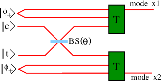
Figure 8: Scheme for a coherent-state CNOT. Target ($\left|t\right\rangle$) and control qubit ($\left|c\right\rangle$) are superimposed at a beam splitter (reflectivity $\cos^{2}(\theta/2)$). The states of the output modes are, then, teleported onto the state of mode $x1$ and $x2$. The boxes labeled $T$ resume the teleportation operations.

Explicitly, the control and target qubits can be written on the $y$ modes of the trapped ions $1$ and $2$. The ECSs we need for the teleportations are codified in the state of the $x$ and $z$ modes. The beam splitter operation between the control and target qubits is, in this case, the sole delocalized operation we need to perform. The scheme we have described for motional-state transfer is exactly what we need to split the input modes in a distributed way. All the other operations do not involve coupling between the ions of the register. The Bell-state measurement is finally performed involving $z$ and $y$ motional modes, projecting the $x$ modes onto a state equivalent to ${\textsf{CNOT}}\left|c,t\right\rangle_{x1,x2}$. We conclude our analysis with a remark concerning the strategy to follow in order to discriminate the logical states of the qubit (namely between $\left|\alpha\right\rangle$ and $\left|-\alpha\right\rangle$). This can be done locally, following ref. jacobmyung , using a $50:50$ BS operation superimposing the state of the qubit, codified in the $x$ mode of an ion, to a coherent state of the ancillary $y$ mode. Then, with proper resonant transitions coupling the internal state of the ion to the $x$ and $y$ modes and highly-efficient electronic state detection, we can ascertain the state of the qubit wineland . The generalization of this procedure to a delocalized situation can be done exploiting the results shown in Section III.

VI Remarks

In this paper we have presented a scheme that, exploiting the motional degrees of freedom of individually trapped ions, could allow for coherent-state quantum computation jacobmyung ; ralph . We have addressed a model for quantum engineering based on the use of two non-resonant laser pulses. By regulating the direction of the lasers along the trap axes and tuning their frequencies to excite proper sidebands, we realize various linear and non-linear interactions, both for the one-qubit and the two-qubit operations. To scale up the dimension of a quantum register, we have considered a distributed design of the quantum computer, each node of the network being a single trapped ion. The interconnections between remote nodes are established by a cavity-bus coupled to the transition of the selected ion  schmidt-kaler ; walther . Motional state transfer, in this way, is shown to be realizable with good fidelity and without the requirement of a high-quality factor cavity. Finally, an efficient quasi-Bell state discrimination is possible, in this set-up, using unitary rotations of the states belonging to the ECS class and inferring the parity eigenvalues of superposition of coherent states via high-efficiency electronic detections. The accuracy of this scheme can be, in principle, arbitrarily near to $100\%$ due to the exploitation of the additional degree of freedom represented by the electronic state of the ion. This feature allows us to circumvent the bottleneck represented by the no-go theorem in ref. norbert . We have addressed the issues of efficiency and practicality of our proposal showing that, singularly taken, each step of the scheme is foreseeable with the current state of the art technology, the main difficulty, up to date, being represented by the sequential combination of them.

- (1) D. Bouwmester, J.-W. Pan, K. Mattle, M. Eibl, H. Weinfurter and A. Zeilinger, Nature 390, 575 (1997); D. Boschi, S. Branca, F. De Martini, L. Hardy and S. Popescu, Phys. Rev. Lett. 80, 1121 (1998); A. Furusawa, J. L. Sorensen, S. L. Braunstein, C. A. Fuchs, H. J. Kimble and E. S. Polzik, Science 282, 706 (2000).
- (2) T. C. Ralph, quant-ph/0306190 (2003).
- (3) E. Knill, R. Laflamme and G. J. Milburn, Nature 409, 46 (2001).
- (4) S. D. Bartlett and B. C. Sanders, Phys. Rev. A, 65, 042304 (2002).
- (5) H. Jeong and M. S. Kim, Phys. Rev. A 65, 042305 (2002).
- (6) http://qist.lanl.gov
- (7) M. Paternostro, M. S. Kim, and B. S. Ham, Phys. Rev. A 67, 023811 (2003); M. Paternostro, M. S. Kim, and B. S. Ham, J. Mod. Opt. 50, 2565 (2003).
- (8) B. Yurke and D. Stoler, Phys. Rev. Lett. 79, 325 (1997); see also V. Bužek and P. L. Knight, in Progress in Optics XXXIV, pp. 1-159, edited by E. Wolf (Elsevier, Amsterdam, 1995) and references within.
- (9) D. J. Wineland, C. Monroe, W. M. Itano, D. Leibfried, B. E. King, and D. M. Meekhof, J. Res. Natl. Inst. Stand. Technol. 103, 259 (1998).
- (10) M. Šašura and V. Bužek, J. Mod. Opt. 49, 1593 (2002).
- (11) J. Steinbach, J. Twamley, and P. L. Knight, Phys. Rev. A 56, 4815 (1997).
- (12) D. Leibfried, D. M. Meekhof, C. Monroe, B. E. King, W. M. Itano and D. J. Wineland, J. Mod. Opt. 44, 2485 (1997).
- (13) G. R. Guthöhrlein, M. Keller, K. Hayasaka, W. Lange, and H. Walter, Nature 414, y49 (2001).
- (14) A. B. Mundt, A. Kreuter, C. Becher, D. Leibfried, J. Eschner, F. Schmidt-Kaler, and R. Blatt, Phys. Rev. Lett. 89, 103001 (2002).
- (15) W. J. Munro, G. J. Milburn, and B. C. Sanders Phys. Rev. A 62, 052108 (2000).
- (16) H. Häffner, S. Gulde, M. Riebe, G. Lancaster, C. Becher, J. Eschner, F. Schmidt-Kaler, and R. Blatt, Phys. Rev. Lett. 90, 143602 (2003).
- (17) P. T. Cochrane, G. J. Milburn, and W. J. Munro, Phys. Rev. A 59, 2631 (1999).
- (18) B. C. Sanders, Phys. Rev. A 45, 6811 (1992).
- (19) We are considering a quadrupole transition in which the ion is coupled to the gradient of the electric field. Thus, the optimal coupling is at the nodes of the field.
- (20) J. I. Cirac, Phys. Rev. A 46, 4354 (1992); M. Paternostro, W. Son, and M. S. Kim, quant-ph/0310031 (2003).
- (21) M. Murao and P. L. Knight, Phys. Rev. A 58, 663 (1998); S. Schneider and G. J. Milburn, Phys. Rev. A 57, 3748 (1998); Ch. Roos, Th. Zeiger, H. Rohde, H. C. Nägerl, J. Eschner, D. Leibfried, F. Schmidt-Kaler, and R. Blatt, Phys. Rev. Lett. 83, 4713 (1999).
- (22) J. I. Cirac, P. Zoller, H. J. Kimble, and H. Mabuchi, Phys. Rev. Lett. 78, 3221 (1997).
- (23) Generally speaking, it is , where is the dimension of the Hilbert-Schmidt space in which is defined. In our case, because of the restriction of the computational basis.
- (24) D. Gottesman and I. L. Chuang, Nature 402, 390 (1999).
- (25) N. Lütkenhaus, J. Calsamiglia, and K.-A. Suominen, Phys. Rev. A 59, 3295 (1999).
- (26) D. Vitali, M. Fortunato, and P. Tombesi, Phys. Rev. Lett. 85, 445 (2000).
- (27) C. W. J. Beenakker and M. Kindermann Phys. Rev. Lett. 92, 056801 (2004); P. G. Kwiat and H. Weinfurter, Phys. Rev. A 58, 2623(R) (1998); C.W.J. Beenakker, D.P. DiVincenzo, C. Emary, M. Kindermann, quant-ph/0401066 (2004).
- (28) R. Blatt and P. Zoller, Eur. J. Phys. 9, 250 (1988).
- (29) An alternative way to discriminate even and odd coherent states requires the Hadamard gate and a beam splitter operation. Indeed, the application of a Hadamard gate (for example the one we have discussed in Section II) to an even (odd) coherent state produces the coherent state (). Mixing this at a beam splitter with another coherent state of amplitude () produces the beam-splitter’s output state . Thus, the distinction between the two class of states reduces to the discrimination between a zero-phonon state and a coherent state of amplitude in the output mode , for example (represented by one of the vibrational modes of the trapped ion) and this can be performed quite efficiently as described in wineland .
- (30) B.-G. Englert, N. Sterpi and H. Walther, Opt. Commun. 100, 526 (1993); Lutterbach and L. Davidovich, Phys. Rev. Lett. 78, 2547 (1997); M. S. Kim and J. Lee, Phys. Rev. A 61, 042102 (2000).
- (31) S. M. Barnett and P. M. Radmore, Methods in Theoretical Quantum Optics (Oxford Univ. Press, 1997).
- (32) T. C. Ralph, A. Gilchrist, G.J. Milburn, W. J. Munro and S. Glancy, Phys. Rev. A 68, 042319 (2003).
- (33) M. J. Bremner, C. M. Dawson, J. L. Dodd, A. Gilchrist, A. W. Harrow, D. Mortimer, M. A. Nielsen, and T. J. Osborne, Phys. Rev. Lett. 89, 247902 (2002).
- (34) J. Zhang, J. Vala, S. Sastry, and K. B. Whaley, Phys. Rev. Lett. 91, 027903 (2003); J. Zhang, J. Vala, S. Sastry, and K. B. Whaley, quant-ph/0308167 (2003).