Entanglement flow in multipartite systems

Abstract

We investigate entanglement dynamics in multipartite systems, establishing a quantitative concept of entanglement flow: both flow through individual particles, and flow along general networks of interacting particles. In the former case, the rate at which a particle can transmit entanglement is shown to depend on that particle’s entanglement with the rest of the system. In the latter, we derive a set of entanglement rate equations, relating the rate of entanglement generation between two subsets of particles to the entanglement already present further back along the network. We use the rate equations to derive a lower bound on entanglement generation in qubit chains, and compare this to existing entanglement creation protocols.

I Introduction

New fields of physics often give rise to new physical quantities to study, and quantum information theory has proved a rich source of study material. As an amalgam of quantum mechanics and information theory, many of the new quantities are quantum analogues of familiar friends from classical information theory: the qubit, for instance, measures quantum information just as the bit measures classical information Schumacher (1995). Other quantities have no obvious classical counterpart. The best-known example is entanglement. Originally seen as the phenomenon that epitomized quantum weirdness, it has become established over the last decade as as a physical quantity, on a par with, say, energy.

The analogy with energy can be pushed quite far: entanglement has a number of similar properties. Like energy, entanglement can be quantified in a meaningful way QIC (2001), allowing us to say that one state is more entangled than another. Like energy, entanglement can be converted from one form to another Nielsen (1999). And like energy, it is a resource that can be used to carry out useful tasks, such as teleportation Bennett et al. (1993).

Until recently, work concentrated on understanding these static properties of entangled quantum states. Although we are some way from a complete understanding of entanglement statics, there has been significant progress: for instance, bipartite pure-state entanglement is now well understood. This begs the question: what happens if we allow the state to evolve?

The move from entanglement statics to entanglement dynamics raises many new and interesting questions. How does entanglement evolve as particles interact Dür et al. (2001)? How good is a particular interaction at creating entanglement Dür et al. (2001); Bennett et al. (2003); Childs et al. (2003)? More generally, how good is an interaction at simulating various non-local processes Khaneja et al. (2001); Bremner et al. (2004)? Or, turning this on its head, how ‘non-local’ is a given process (e.g. a quantum gate) Vidal et al. (2002); Zanardi et al. (2000)? This article extends the first of these — how entanglement evolves as particles interact — to multipartite systems.

The Schrödinger equation already implicitly describes the complete dynamics of a quantum system, but to gain insight into entanglement dynamics, we need equations that explicitly involve the entanglement of the system, without reference specific features of the Hamiltonian. One of the first steps along this path was taken by Dür et. al.  who investigated the rate of entanglement generation in two-qubit systems Dür et al. (2001). They derived an equation relating the rate of entanglement creation to the existing entanglement in the system, along with a factor depending on the form and strength of the interaction. This latter led to a pleasingly simple quantity measuring the entanglement generating capacity of two-qubit interactions Bennett et al. (2003); Childs et al. (2003).

In a system of two particles coupled by a Hamiltonian, the only entanglement dynamics that can take place is creation of entanglement between the two particles. A simple tripartite system already raises other interesting questions. For instance, in a chain of three particles, how does entanglement ‘flow’ through the middle one? Surprisingly, we showed in previous work Cubitt et al. (2003) that, in just such a chain, entanglement can be created between the two end particles, without the middle particle ever becoming entangled. This would seem to put an end to notions of entanglement ‘flow’. However, we also gave a simple proof that this phenomenon is only possible for mixed initial states; for pure states, the middle particle necessarily becomes entangled during the evolution.

This suggests there is a connection between pure-state entanglement of a mediating particle and entanglement flow through that particle: if it is not entangled, no entanglement flows. In section II, we show that there is indeed a quantitative relation describing how the entanglement of a particle with the rest of the system limits the flow of entanglement through that particle. We first consider a three-qubit system, before dealing with general systems. The concept of entanglement flow through particles is therefore put on a quantitative footing for systems in pure states. This contrasts strongly with the mixed-state case, in which entanglement can seemingly ‘tunnel’ through mediating systems.

Flow through individual particles is one aspect of entanglement dynamics in multipartite systems. But in a network of many interacting particles, we may also be interested in how entanglement flows along the whole network. We develop these ideas in the second half of this article.

The inspiration is loosely based on the Arrhenius equations for chemical reactions. The reaction mechanism of a chemical reaction describes the steps by which reactants are transformed, via successive intermediate compounds, into the final products. The rate at which a compound is produced depends on the amounts of its immediate precursors that are present. Thus the complete reaction is described by a set of coupled rate equations, one for each step in the reaction mechanism.

In section III, we derive a set of differential equations describing entanglement flow, analogous to the rate equations for a chemical reaction. The rate at which entanglement is generated between two sets of particles is shown to depend on the amount of entanglement already present further back along the network. The entanglement dynamics of the complete system is described by a coupled set of such entanglement rate equations, one for each step in the interaction network.

Unlike the equations describing flow through individual particles, these entanglement rate equations apply equally well to both pure and mixed states. Therefore, they establish a concept of entanglement flow along general networks of interacting particles (even though the concept of flow through individual particles in the system may be meaningless).

In section IV, we apply our new understanding of entanglement flow to investigate entanglement generation in chains of interacting particles. First, we briefly review some existing entanglement generation protocols for qubit chains, in the context of the rate equations derived in section III. Finally, we use the rate equations to prove a universal lower bound on the time it takes to create entanglement, or more precisely the scaling of this with the length of the chain (the results can easily be extended to general networks).

II Flow through particles

In this section, we will investigate entanglement flow through mediating particles. Specifically, we will consider flow through the middle particle in tripartite chains. The results of Cubitt et al. (2003) show that this concept does not make sense if the whole system is in a mixed state. But for pure states, the rate at which entanglement is generated between the end particles is indeed zero if the middle particle is not entangled.

The latter is suggestive: is there a general quantitative relationship between the entanglement of a particle, and the rate at which entanglement can flow through it, for systems in pure states? If the middle particle is only slightly entangled, does entanglement flow only slowly? We will derive just such a relationship, first for the simplest tripartite system: a three-qubit chain, then for general tripartite chains.

When investigating (bipartite) entanglement flow through mediating particles in more general settings, the system can always be described as a tripartite chain: the mediating particles form one party, and the sets of particles each side, which are becoming entangled, form the other two. Thus the equation for tripartite chains can in fact be applied generally to describe entanglement flow through mediating systems.

II.1 The three-qubit chain

Consider a chain of three qubits, labeled $a$, $b$, and $c$, with nearest neighbour interactions described by Hamiltonians $H_{ab}$ and $H_{bc}$. We will restrict the overall state of the system, $\mathinner{|\psi\rangle}_{abc}$ to be pure. However, the reduced state of the two end qubits, $\rho_{ac}$, need not remain pure during the evolution (if $b$ is to become entangled at any point, $\rho_{ac}$ will necessarily become mixed). To quantify the entanglement between $a$ and $c$, we need an entanglement measure valid for mixed states. The natural choice is the concurrence Wootters (1998). Though it is an entanglement measure in its own right, its interest lies in its is equivalence to one of the important, physically meaningful entanglement measures: the entanglement of formation Bennett et al. (1996).

We can write the overall state of the system in its Schmidt decomposition with respect to the partition $(b:ac)$: $\mathinner{|\psi\rangle}_{abc}=\lambda_{1}\mathinner{|\varphi_{1}\rangle}_{ac}\mathinner{|\chi_{1}\rangle}_{b}+\lambda_{2}\mathinner{|\varphi_{2}\rangle}_{ac}\mathinner{|\chi_{2}\rangle}_{b}$. The Schmidt coefficients, $\lambda_{1}$ and $\lambda_{2}$, determine the non-local properties of the state with respect to this partition, including entanglement of the middle qubit $b$ with the rest. Meanwhile, the entanglement of the reduced state of the end two qubits, $\rho_{ac}$, can be measured by the concurrence, denoted $C_{ac}$. Following Audenaert et al. (2001), the state of particles $a$ and $b$ can be represented by a $4\times 2$ matrix $X=(\lambda_{1}\mathinner{|\varphi_{1}\rangle},\lambda_{2}\mathinner{|\varphi_{2}\rangle})$. The concurrence can be calculated from the singular values $\varsigma_{1}\geq\varsigma_{2}$ of $A=X^{T}\Sigma X$, where $\Sigma=\sigma_{y}\otimes\sigma_{y}$: $C_{ac}=\varsigma_{1}-\varsigma_{2}=\sqrt{\operatorname{tr}A^{\dagger}A-2|\det A|}$. Taking the time-derivative of this and simplifying the resulting exact expression (see Appendix A for details) leads to the following bound on the entanglement rate:

$$\frac{\mathrm{d}C_{ac}^{2}}{\mathrm{d}t}\leq 8\left\|H\right\|\lambda_{1}\lambda_{2}.$$

The factor $||H||=||H_{ab}||_{1}+||H_{bc}||_{1}$ measures the strengths of the interactions. $||H||_{1}=\sum_{ij}|H_{ij}|$ denotes the $l_{1}$ norm, where the Hamiltonians are written in the product basis $H=\sum_{ij}H_{ij}\sigma_{i}\otimes\sigma_{j}$, and the Pauli matrices $\sigma_{1,2,3}=\sigma_{x,y,z}$ are defined in the Schmidt basis $\{\mathinner{|\chi_{1}\rangle}\mathinner{|\chi_{2}\rangle}\}$. (Local terms $\sigma_{i}\otimes\mathbbm{1}$ or $\mathbbm{1}\otimes\sigma_{j}$ in the Hamiltonian can not alter the entanglement of the system, so do not contribute).

In the context of entanglement dynamics, the important part of the relation is the product of Schmidt coefficients $\lambda_{1}\lambda_{2}$, which is a pure-state bipartite entanglement measure. (In fact, up to a numerical factor, it is the concurrence.) Thus the differential equation tells us that the entanglement of the middle qubit limits entanglement generation between the end qubits: not only must $b$ be entangled for entanglement to be generated between $a$ and $c$ (precisely what was shown not to hold for mixed states in Cubitt et al. (2003)), but the rate at which it is generated can be larger the more entangled $b$ is.

At first sight, the inequality may appear too weak, as it does not seem to imply that the derivative is zero once qubits $a$ and $c$ are maximally entangled. However, $C_{ac}$ and $\lambda_{1}\lambda_{2}$ are not independent quantities. When $a$ and $c$ are maximally entangled, they can not be entangled with anything else, thus $\lambda_{1}\lambda_{2}=0$, and the derivative is zero after all.

A complete quantitative description of entanglement creation in the three-qubit chain would require an equation describing the evolution of the Schmidt coefficients. However, $(b:ac)$ forms a bipartite, pure-state system. Entanglement creation in bipartite systems and the evolution of the Schmidt coefficients has been investigated in Dür et al. (2001).

II.2 Fidelities and entangled fractions

The three-qubit result can not directly be extended to higher dimensional systems. Whilst we can restrict the system to pure states for the same reasons as in the three-qubit case, the reduced density matrix of the two end particles can again become mixed during the evolution. And no closed-form expression is known for the entanglement of formation of mixed states, other than in the two-qubit case.

Before turning to higher-dimensional systems, it is instructive to consider more carefully the setting in which we wish to investigate entanglement dynamics. Entanglement measures are defined in the LOCC paradigm: local operations and classical communication (LOCC) can only decrease the entanglement of a state. This is the natural paradigm when thinking about entanglement from an information-theorist’s point of view, in which entangled states are shared between different parties who are free to act locally on their part of the state.

But we are considering entanglement dynamics from a physical standpoint. In a system of interacting particles, it is not clear what classical communication means. Any transfer of classical information between particles would still have to take place via the (quantum) interactions. It could be argued that it makes more sense in this context to define entanglement in the local-unitary paradigm: any change to a state due to local terms in the interaction Hamiltonian should not change the entanglement.

A physical way of measuring entanglement in this paradigm is to use the fidelity Jozsa (1994), which measures the distance between states . The entangled fraction of a state $\rho$ is then defined as the maximum fidelity with a maximally entangled state:

$$F(\rho):=\max_{\mathinner{|\phi\rangle}\in M.E.}\raisebox{-3.00003pt}{$\scriptstyle{}$}\left<\phi\right|\rho\left|\phi\right>,$$

where the maximization is over all maximally entangled states $\mathinner{|\phi\rangle}$ in the bipartite Hilbert space of $\rho$. (For two-qubit states, it is also called the singlet fraction.) It measures how close a given state is to any maximally entangled state, and is invariant under local unitary operations, as required.

The entangled fraction is also an experimentally relevant quantity. When trying to engineer an evolution to produce a particular state (a highly entangled one, for instance), we want to know how close the actual state is to the desired one — precisely what is measured by the fidelity. For example, in teleportation experiments, it is the entangled fraction of the entangled pair that determines how close the teleported state is to the original Horodecki et al. (1999).

Therefore, in the remainder of this article, we will consider evolution of the entangled fraction and related quantities. Though it is a well-motivated quantity to study in its own right, it can also be used to give upper and lower bounds on entanglement measures such as the concurrence Verstraete and Verschelde (2002) (and hence entanglement of formation). In particular, if a state is separable, its entangled fraction is less than or equal to $1/n$ (with $n$ the dimension of the smaller of the two Hilbert spaces making up the bipartite space). Whereas if (and only if) the entangled fraction is equal to one, the state must be maximally entangled.

In the final section, we will use our results to derive bounds on how long it takes to entangle particles when the system starts in a separable state. In this context, any quantity that takes different values for separable and maximally entangled states is equally good in principle: we can bound the time required to change from one value to the other. The entangled fraction, for example, must increase from $1/n$ to $1$.

II.3 General tripartite chains

The tripartite chain is a prototype for all indirect (bipartite) entanglement creation. We can always divide a system into three: two systems that are being entangled, and everything else lumped into one mediating system. We can then investigate entanglement flow through this mediating system.

In a general tripartite chain, consisting of systems $A$, $B$ and $C$ of arbitrary dimension, interacting by nearest-neighbour interactions $H_{AB}$ and $H_{BC}$, the Schmidt decomposition has the form $\mathinner{|\psi\rangle}_{ABC}=\sum_{i}\lambda_{i}\mathinner{|\psi_{i}\rangle}_{AC}\mathinner{|i\rangle}_{B}$, where we sort the Schmidt coefficients $\lambda_{i}$ in descending order. By re-expressing the entangled fraction as a maximization over purifications using Uhlmann’s Theorem (see Appendix B), we can derive an exact expression for the time derivative of the entangled fraction. Simplifying the exact result to separate out the entanglement dependence yields a relation analogous to the three-qubit case (see Appendix C for details):

$$\dot{F}(\rho_{AC})\leq 2\left|H\right|\sqrt{F(\rho_{AC})}\,\Bigl{(}\sum_{ij}\lambda_{i}\lambda_{j}-\lambda_{1}^{2}\Bigr{)}$$

Again, the factor $\left|H\right|=\left|H_{AB}\right|_{\infty}+\left|H_{AB}\right|_{\infty}$ measures the interaction strengths, independent of the system state ($|H|_{\infty}=\max_{ij}|H_{ij}|$ denotes the $l_{\infty}$ norm).

The quantity in brackets is closely related to the entangled fraction of $\mathinner{|\psi\rangle}_{ABC}$ in the $(B:AC)$ partition: $F(\mathinner{|\psi\rangle\raisebox{-3.00003pt}{$\scriptstyle$}\langle\psi|})=\tfrac{1}{n}\sum_{ij}\lambda_{i}\lambda_{j}$ (with $n$ the smaller of the dimensions of $B$ and $AC$). Subtracting $\lambda_{1}^{2}$ re-scales this entangled fraction so that it is zero when the state is separable. Therefore, the entanglement of $B$ with the rest of the system limits the rate at which entanglement can flow through $B$. As in the three-qubit case, the derivative implicitly goes to zero when systems $A$ and $C$ become maximally entangled, since they can not then be entangled with $B$.

III Flow along networks

In the previous section, we examined entanglement flow through the middle particle in a tripartite chain, and noted that the results can be applied to flow through individual particles in general systems, by viewing the system as a tripartite chain. However, in a large multipartite system, this approach means lumping many particles together into single composite particles, hiding much of the entanglement dynamics. Can we more fully describe entanglement flow in networks of interacting particles?

In this section, we derive a set of differential equations describing the entanglement dynamics, analogous to the rate equations for a chemical reaction. These show that the rate at which entanglement is created between two sets of particles depends on the existing entanglement further back along the network. Intuitively, this can be interpreted as entanglement flowing through the network.

III.1 Generalized singlet fraction

As in the previous section, we must first address the problem of how to measure entanglement in large systems. Even before that, we must decide what entanglement to measure, since multipartite systems provide a plethora of possibilities. What questions are we interested in investigating using our putative equations? Perhaps the most natural goal, given a system of many interacting particles, is to entangle a particular pair of them: the end qubits in a chain, for example. We will take this as our motivation for again considering entangled fractions of the two particles. We will also need to define a new fidelity-based quantity to measure bipartite entanglement embedded in larger systems.

First note that, since any maximally entangled state can be reached by acting with local unitaries on a particular maximally entangled state, we can of course maximize over unitaries rather than states in the definition of the entangled fraction:

$$F(\rho)=\max_{U_{a},U_{b}}\raisebox{-3.00003pt}{$\scriptstyle{}$}\left<\phi\right|U_{a}^{\dagger}\otimes U_{b}^{\dagger}\,\rho_{ab}\,U_{a}\otimes U_{b}\left|\phi\right>$$

We can equally well think of the unitaries as acting on $\rho$ rather than on the entangled state $\mathinner{|\phi\rangle}_{ab}$. This suggests an alternative interpretation of the singlet fraction: as the maximum fidelity with a particular maximally entangled state (e.g. the singlet) that can be achieved by acting with local unitaries.

Based on this interpretation, we define the generalized singlet fraction, a measure of two-qubit entanglement for bipartite systems of arbitrary dimension (it can be extended in the obvious way to measure general bipartite entanglement not (a)):

$$F(\rho_{AB})=\max_{U_{A},U_{B}}\raisebox{-3.00003pt}{$\scriptstyle{}$}\left<\phi\right|\operatorname{tr}_{\!/\!ab}(U_{A}\otimes U_{B}\;\rho_{AB}\;U_{A}^{\dagger}\otimes U_{B}^{\dagger})\left|\phi\right>,$$ (1)

where $a$ and $b$ are qubit systems embedded in $A$ and $B$ respectively, $\mathinner{|\phi\rangle}_{ab}$ is the singlet state, and the notation $\operatorname{tr}_{\!/\!ab}$ indicates the partial trace over all systems other than $a$ and $b$. It measures the maximum fidelity with the singlet achievable by local unitaries.

Note that, in two-qubit systems, this generalized singlet fraction reduces to the usual singlet fraction. For any system, it takes values between 0 and 1, and for separable states it is less than or equal to $1/2$. Also, from the definition, if $A$ and $B$ are subsystems of $A^{\prime}$ and $B^{\prime}$, so that $\rho_{AB}=\operatorname{tr}_{\!/\!AB}(\rho_{A^{\prime}B^{\prime}})$, then $F(\rho_{AB})\leq F(\rho_{A^{\prime}B^{\prime}})$.

III.2 Entanglement rate equations

We are now ready to state our main result: a set of coupled differential equations describing entanglement flow in networks of interacting particles. For simplicity, we assume that among the set of interacting particles $S$, there are at least two qubits $a$ and $b$, the premise being that we are interested in entangling these. (The results can easily be generalized: see not (a) and Conclusions.) Let $A$ and $B$ be disjoint subsets of $S$. The equations describe the rate at which the generalized singlet fraction of $\rho_{AB}$ can increase.

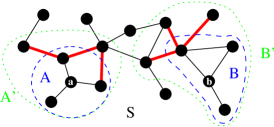
Figure 1: A network of interacting particles, showing interactions and sets defined in the entanglement rate equations. Interactions ‘crossing the boundaries’ of $A$ or $B$ are indicated by thicker lines.

Define $A^{\prime}$ and $B^{\prime}$ to be the sets of particles directly connected by an interaction to at least one particle in $A$ or $B$ respectively (i.e. $A^{\prime}$ is the set of particles at most ‘one-away’ from $A$, thus $A\subseteq A^{\prime}$; see Fig 1). If $A^{\prime}$ and $B^{\prime}$ are disjoint (as in Fig. 1), then the time derivative of the generalized singlet fraction is bounded by

$$\dot{F}(\rho_{AB})\leq 2\left\|H\right\|\sqrt{F(\rho_{AB})}\sqrt{F(\rho_{A^{\prime}B^{\prime}})-F(\rho_{AB})},$$ (2a)

whilst if $$A^{\prime} B^{\prime}$$ and have one or more particles in common, then

$$\dot{F}(\rho_{AB})\leq 2\left\|H\right\|\sqrt{F(\rho_{AB})}\sqrt{1-F(\rho_{AB})}.$$ (2b)

The factor $\left\|H\right\|$ is a sum of strengths of those interactions that connect a particle in $A$ or $B$ to one outside $A$ or $B$ respectively (i.e. interactions that ‘cross the boundary’ of $A$ or $B$; see Fig. 1):

$$\left\|H\right\|=\sum_{\mathchoice{\hbox to0.0pt{\hss$\displaystyle{\begin{subarray}{c}i\in A,j\notin A;\\ i\in B,j\notin B\end{subarray}}$\hss}}{\hbox to0.0pt{\hss$\textstyle{\begin{subarray}{c}i\in A,j\notin A;\\ i\in B,j\notin B\end{subarray}}$\hss}}{\hbox to0.0pt{\hss$\scriptstyle{\begin{subarray}{c}i\in A,j\notin A;\\ i\in B,j\notin B\end{subarray}}$\hss}}{\hbox to0.0pt{\hss$\scriptscriptstyle{\begin{subarray}{c}i\in A,j\notin A;\\ i\in B,j\notin B\end{subarray}}$\hss}}}\left\|H_{ij}\right\|_{HS},$$

where $\left\|\,\bullet\right\|_{HS}$ denotes the Hilbert-Schmidt norm.

The first step in the proof of these entanglement rate equations to rewrite the generalized singlet fraction (1) in terms of purifications of $\rho_{AB}$ using Uhlmann’s theorem (Appendix B). This leads to the following exact expression for the derivative of the generalized singlet fraction:

$$\dot{F}(\rho_{AB})=\sqrt{F(\rho_{AB})}\cdot\max_{\begin{subarray}{c}U_{A},U_{B}\\ \mathinner{|\chi\rangle}\end{subarray}}\frac{1}{i}\sum_{\mathchoice{\hbox to0.0pt{$\displaystyle{\begin{subarray}{c}i\notin A(B)\\ j\in A(B)\end{subarray}}$\hss}}{\hbox to0.0pt{$\textstyle{\begin{subarray}{c}i\notin A(B)\\ j\in A(B)\end{subarray}}$\hss}}{\hbox to0.0pt{$\scriptstyle{\begin{subarray}{c}i\notin A(B)\\ j\in A(B)\end{subarray}}$\hss}}{\hbox to0.0pt{$\scriptscriptstyle{\begin{subarray}{c}i\notin A(B)\\ j\in A(B)\end{subarray}}$\hss}}}\raisebox{-3.00003pt}{$\scriptstyle{}$}\left<\varphi\right|H_{ij}\left|\psi\right>-\raisebox{-3.00003pt}{$\scriptstyle{}$}\left<\psi\right|H_{ij}\left|\varphi\right>$$

where $\mathinner{|\psi\rangle}$ is a purification of $\rho_{AB}$, $\mathinner{|\chi\rangle}$ is an extension of the singlet state to the Hilbert space of $\mathinner{|\psi\rangle}$, and $\mathinner{|\varphi\rangle}=U_{A}^{\dagger}\otimes U_{B}^{\dagger}\mathinner{|\chi\rangle}$. Using Lemma 3 (Appendix B), the terms inside the sum can be bounded by $\frac{1}{i}(\raisebox{-3.00003pt}{$\scriptstyle{}$}\left<\varphi\right|H_{ij}\left|\psi\right>-\mathrm{h.c.})\leq 2\left\|H_{ij}\right\|_{\mathrm{HS}}\sqrt{(\operatorname{tr}\left|X_{ij}\right|)^{2}-(\operatorname{tr}(\operatorname{Re}X_{ij}))^{2}}$, where $X_{ij}=\operatorname{tr}_{\!/\!ij}\left|\psi\vphantom{\varphi}\right>\raisebox{-3.00003pt}{$\scriptstyle$}\left<\varphi\vphantom{\psi}\right|$. Finally, the quantities under the square-root can be related to generalized singlet fractions: $(\operatorname{tr}(\operatorname{Re}X_{ij}))^{2}=F(\rho_{AB})$ and $\operatorname{tr}(\left|X_{ij}\right|)^{2}\leq F(\rho_{A^{\prime}B^{\prime}})$, which concludes the proof. (The proof is given in full detail in Appendix B).

We can gain some insight into entanglement dynamics by considering the qualitative meaning of the rate equations, before thinking about solving them. They divide a network of interacting particles into pairs of concentric sets, surrounding qubits $a$ and $b$. For example, in Fig. 1 there are three such pairs: the qubits $a$ and $b$ themselves, the sets labeled $A$ and $B$, and those labeled $A^{\prime}$ and $B^{\prime}$. The rate equations tell us that entanglement must first build up between the largest sets, before it can cascade down successively smaller ones, finally reaching the two qubits (just as in a chemical reaction, intermediate compounds in the reaction mechanism must be created before the final product is reached). What is more, the rate at which the entanglement flows from one level to the next depends on the difference in entanglement between the two levels (somewhat like the rate of a reversible chemical reaction, which depends on the difference between the concentrations of reactants and products; or like flow in fluids, in which the flow rate depends on the pressure difference).

The number of pairs of sets is equal to half the ‘interaction distance’ of the two qubits (rounded down to the nearest integer), i.e. half the smallest number of links in the network needed to connect $a$ to $b$ (in Fig. 1, their interaction distance is 5). A generalized singlet fraction can be defined on each pair of sets, along with an accompanying rate equation describing its evolution. Therefore any network has the same rate equations as a chain whose length is equal to the interaction distance, and whose interaction strengths along each link of the chain equal the factors $||H||$; all entanglement flow is equivalent to flow along a chain. This is qualitatively similar to results from quantum random walks, in which a quantum walk over a network is equivalent to a quantum walk along a chain Farhi and Gutmann (1998).

Note that the factor $||H||$ in the rate equations indiscriminately includes all interactions that cross the boundary. We might expect different interactions to contribute differently, depending on their location in the network. In fact, in Appendix B, we derive a more general version of the rate equations, which accounts for each possible interaction pathway separately, and can therefore take into account the different roles different particles play in the entanglement dynamics, due to their differing connectivity. The inequality in the corresponding rate equations is therefore tighter, but it leads to exponentially (in the number of particles) more equations describing the entanglement dynamics of a system, and gives a less intuitive picture of entanglement flow. We will find that the simpler form given here is sufficient to derive a number of interesting results.

III.3 Limits from the rate equations

It is straightforward to prove inductively that the curves produced by saturating the inequalities in the rate equations (2a,2b) constitute upper bounds on the evolution of the generalized singlet fractions; i.e. the fastest possible evolution allowed by the rate equations is that which saturates the rate equations at each point in time.

If the interaction distance between the qubits we intend to entangle is $d$, then the full set of rate equations involve $\lfloor d/2\rfloor$ generalized singlet fractions, which we will denote $F_{k}(t)$, $k=1\dots\lfloor d/2\rfloor$. ($\lfloor\bullet\rfloor$ denotes rounding down to the nearest integer.) We number them such that $F_{\lfloor d/2\rfloor}$ is the singlet fraction of the two qubits. If we define $F_{0}=1$, then the evolution of each $F_{k}(t)$ is described by equation (2a).

Let $f_{k}(t)$ be the curves that saturate the rate equations, i.e. $f_{k}(t)$ is the solution to

$$\dot{f_{k}}=2\left\|H\right\|\sqrt{f_{k}}\sqrt{f_{k-1}-f_{k}},$$

with $f_{0}=1$. (For simplicity, we can take all coupling strengths $||H||$ to be 1.) Assume that $f_{k}(t)$ is an upper bound on $F_{k}(t)$, i.e. $f_{k}(t)\geq F_{k}(t)$ for all $t$. If $f_{k+1}(t)$ is not an upper bound on $F_{k+1}(t)$, then $F_{k+1}(t)$ must cross it at some point. If this occurs at $t=t_{0}$, then $F_{k+1}(t_{0})=f_{{k+1}}(t_{0})$ and $\dot{F}_{k+1}(t_{0})>\dot{f}_{k+1}(t_{0})$ . But $F_{k+1}(t)$ must still satisfy the inequality in equation (2a). Thus

$$\dot{F}_{k+1} \leq 2\sqrt{F_{k+1}(t_{0})}\sqrt{F_{k}(t_{0})-F_{k+1}(t_{0})}$$

$$\leq 2\sqrt{f_{k+1}(t_{0})}\sqrt{f_{k}(t_{0})-f_{k+1}(t_{0})}=\dot{f}_{k+1}(t_{0}),$$

which contradicts the assumption that $F_{k+1}(t)$ crosses $f_{k+1}(t)$ at $t_{0}$. Thus if $f_{k}(t)$ is an upper bound, then so is $f_{k+1}(t)$.

The initial step in the induction (that $f_{1}(t)$ is an upper bound) follows from the second of the rate equations (2b), and the fact that the generalized singlet fraction is upper bounded by 1. Fig. 2 shows numerically calculated curves $f_{k}(t)$ saturating the rate equations.

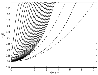
Figure 2: Numerically calculated generalized singlet fraction curves $f_{k}(t)$ saturating the inequalities in the entanglement rate equations (2a,2b). The final solid curve is for $k=50$, i.e. the singlet fraction of the end qubits in a separated by an interaction distance $d=100$. (The dashed curves show the corresponding upper and lower bounds $u_{k}(t)$ and $l_{k}(t)$ for $k=50$, from subsection IV.2).

IV How fast can entanglement be created?

How fast can entanglement be generated in a system of interacting particles? The question is both theoretically interesting, and experimentally important. Many quantum information processing tasks require entanglement, and the faster this can be produced, the less the system will suffer from decoherence. Quantum computing algorithms often generate large amounts of entanglement during their execution, so determining how fast entanglement can be generated can also provide bounds on algorithm complexity Ambainis (2002).

In this section, we briefly review some existing entanglement generation schemes in the context of the entanglement rate equations derived in the previous section. We then investigate what universal limits the rate equations put on how fast entanglement can be generated, or more precisely, how the time required to entangle two particles scales with the size of the system.

IV.1 Entanglement generation schemes

How fast entanglement can be generated depends, of course, on how we are able to manipulate the system. For definiteness, consider entanglement generation in a qubit chain. It turns out that measurement is a very powerful resource. If we are able to carry out local operations on any qubit, including local measurements and classical communication of the outcomes, then the end qubits in a chain can be maximally entangled in a time independent of the length of the chain. Though not discussed in the context of entanglement generation, Briegel and Raussendorf Briegel and Raussendorf (1002) showed that a cluster state can be created in a chain in constant time, and local measurements on a cluster state allow a Bell-state to be projected out on any desired pair of qubits, including the end pair Verstraete et al. (2004).

The constant scaling assumes we neglect the the time required for classical communication of the measurement outcomes to the ends of the chain. This can be justified on theoretical grounds, since classical communication can not create entanglement, and it makes sense to consider the interactions as the resource. In many physical implementations, it is also reasonable on pragmatic grounds: classical communication is usually much easier to implement than quantum processes. However, if the interactions are really the only non-local resource, then classical communication must also be implemented via the chain, and local measurements are of no benefit, which is equivalent to the local-control scenario described below. This might be the relevant scenario, for instance, for quantum computers.

If we can apply local unitary operations on any qubit in the chain, but not measurements, then we can efficiently simulate evolution under any Hamiltonian (this is true for general systems of interacting particles, not just for qubit chains Nielsen et al. (2002); Wocjan et al. (2002)). Again, it is reasonable to discount local resources, which in this scenario means neglecting the time required to carry out the local unitaries (the ‘fast local unitary’ approximation). And again, this can also be justified on physical grounds, since local unitaries are typically much faster than interactions.

Khaneja and Glaser have developed an interesting protocol for state transfer in this scenario Khaneja and Glaser (2002), in the context of NMR spectroscopy, which can easily be transformed into an entanglement generation protocol. First the middle qubits are entangled, then the state of each middle qubit is encoded into a three-qubit state. The encoded states are transferred along the chain towards the ends, where they are decoded again. The protocol requires local unitaries to be applied at discrete times. The evolution of the generalized singlet fractions is shown in Fig 3, clearly reflecting the fact that the protocol is based on moving states step-by-step along the chain. It achieves a surprising three-fold speedup over the trivial swapping protocol for entanglement generation in a chain (entangle the middle qubits; move to the ends by swapping), though the scaling of the time with the length of the chain is still linear, as in the trivial protocol. In the next subsection, we will use the entanglement rate equations to derive a lower bound on the scaling in this local-control scenario.

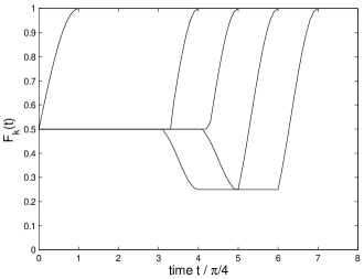
Figure 3: Entanglement dynamics in the entanglement generation protocol based on Khaneja and Glaser’s state transfer scheme Khaneja and Glaser (2002), for a chain of 10 qubits. Successive curves show the evolution of generalized singlet fractions $F_{1}$ through $F_{5}$, numbered as in subsection III.3.

Finally, we may have no local control over the qubits, only retaining the ability to switch on interactions in the entire chain, and switch them off at some later time. Christandl et. al. developed a state-transfer protocol for qubit chains in this scenario Christandl et al. (2003), and Yung et. al. have given a simple extension to entanglement generation Yung et al. (2003). The only local control required is fixing the coupling strengths between different qubits, which must be inhomogeneous. Fig. 4 shows the entanglement dynamics for the odd chain-length protocol of Ref. Yung et al. (2003) — very different to that of Fig. 3. If the strongest coupling strength is normalized to some fixed value, then the time to create a maximally entangled pair again scales linearly with the length of the chain not (b).

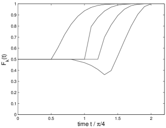
Figure 4: Entanglement dynamics in the entanglement generation scheme for odd chain lengths from Ref. Yung et al. (2003), here for 9 qubits. Successive curves show the evolution of generalized singlet fractions $F_{1}$ through $F_{4}$, numbered as in subsection III.3. (Note that times are not comparable to those in Fig. 3, since interaction strengths in Yung et al. (2003) are not normalized).

Osborne and Linden have also developed a protocol for state transfer in qubit chains, which could be adapted to entanglement generation, involving limited local control over a vanishingly small (in the limit of large chain lengths) number of qubits at each end of the chain Osborne and Linden (2003).

IV.2 Bounds on entanglement generation

In this subsection, we will use the entanglement rate equations to derive a lower bound on how the time to create a maximally entangled state scales with the size of the system.

Unfortunately, the set of differential equations defined by the rate equations (2a,2b) has no known closed-form analytic solution (at least, none that we could find in the literature). Solving numerically can provide numerical bounds on the time required for entanglement generation (see Fig. 2). The interesting question, though, is how this time scales with the size of the system (for instance, the length of a chain), which requires an analytic result.

For simplicity, we will derive a bound on the scaling of the time to entangle the end qubits in a chain of length $L$. The $\lfloor L/2\rfloor$ generalized singlet fractions $F_{k}$ will be numbered such that $F_{\lfloor L/2\rfloor}$ is the singlet fraction of the end two qubits. We assume all interaction strengths are equal to 1, and that the chain is initially in a completely separable pure state (thus $F_{k}(t=0)=1/2$ for all $k$). The result can easily be generalized to different interaction strengths, and indeed to general networks of particles (c.f. discussion in subsection III.2).

We are interested in the time at which $F_{\lfloor L/2\rfloor}$ (the singlet fraction of the two end qubits) reaches 1, as a function of $L$. Though the rate equations do not have an analytic solution, we can inductively prove a bound on the scaling of this time with $L$, using an argument similar to that used in subsection III.3.

There, we showed that the curves obtained when the inequalities in the rate equations are saturated give upper bounds on the evolution of the generalized singlet fractions. We can use the same argument to prove that we still get upper bounds if we weaken the inequalities, using the fact that $F_{k}(t)\leq 1$, and instead solve

$$\dot{f}_{k}(t)=2\sqrt{f_{k-1}(t)-f_{k}(t)}.$$

We can use the argument a third time to prove that if $u_{k}(t)$ is an upper bound on the new $f_{k}(t)$, then the solution $u_{k+1}(t)$ to

$$\dot{u}_{k+1}(t)=2\sqrt{u_{k}(t)-u_{k+1}(t)}$$ (3)

is an upper bound on $f_{k+1}(t)$. I.e. we have $u_{k}(t)\geq f_{k}(t)\geq F_{k}(t)$. (As concerns boundary conditions, we simply require that $u_{k+1}(0)\geq f_{k+1}(0)=F_{k+1}(0)=1/2$.)

Now assume there is a $u_{k}(t)$ of the form

$$u_{k}(t)=\frac{t^{2}}{a_{k}}+\frac{1+\epsilon}{2}$$ (4)

that is an upper bound on $f_{k}(t)$ for some positive constants $a_{k}$ and $\epsilon$. The differential equation for $u_{k+1}(t)$ then has a solution of the same form as $u_{k}(t)$ (as can be seen by direct substitution), with $a_{k+1}$ given by the recursion relation

$$a_{k+1}=\frac{a_{k}}{2}+\frac{a_{k}}{2}\sqrt{1+\frac{4}{a_{k}}}.$$

Since $u_{k+1}(0)=(1+\epsilon)/2$, which is greater than the initial condition $f_{k+1}(0)=F_{k+1}(0)=1/2$, $u_{k+1}(t)$ is an upper bound on $f_{k+1}(t)$ by the argument above.

All that remains is the initial step in the induction: that there is indeed a bound $u_{1}(t)$ on $f_{1}(t)$ with the form assumed in (4), for some constants $a_{1}$ and $\epsilon$. Fortuitously, the differential equation (2b) for $F_{1}(t)$ (the generalized singlet fraction of the entire chain, split into two halves) can be solved analytically when the inequality is saturated (and without weakening the inequality). The solution has the form

$$f_{1}(t)=\sin^{2}(t+\phi)$$

with $\phi$ an arbitrary constant. There is also a trivial solution: $f_{1}(t)=1$. Since the chain starts in a completely separable pure state, the initial condition is $f_{1}(0)=1/2$, and the solution we require is

$$f_{1}(t)=\begin{cases}\sin^{2}(t+\pi/4)&t\leq\pi/4\\ 1&t>\pi/4\end{cases}$$

The two parts to the solution merely reflect the fact that once the generalized singlet fraction has reached its maximum value of 1, there is nothing to be gained by further interaction, and the interactions affecting $F_{1}$ (namely the interactions in the middle of the chain) should be switched off.

Knowing an explicit solution for $f_{1}(t)$, it is easy to find a bound $u_{1}(t)$ with the appropriate form. To make the algebra simpler, we can upper-bound $f_{1}(t)$ by $t+1/2$. Thus a $u_{1}(t)$ with the form given in (4) that satisfies $u_{1}(t)\geq t+1/2$ will suffice to complete the proof. This leads to the relation $a_{1}\leq 2\epsilon$. Any positive $a_{1}$ and $\epsilon$ satisfying this will give an appropriate $u_{1}(t)\geq f_{1}(t)\geq F_{1}(t)$, and will guarantee that $u_{1}(0)=(1+\epsilon)/2\geq f_{1}(0)=F_{1}(0)=1/2$. Therefore we have shown that an upper bound on $F_{1}(t)$ with the appropriate form exists, which completes the proof. For neatness, we can let $\epsilon\rightarrow 0$, so that $u_{k}(0)\rightarrow F_{k}(0)=1/2$ and $a_{0}\rightarrow 0$ (as used to give the curve $u_{50}(t)$ shown in Fig. 2).

Solving $u_{\lfloor L/2\rfloor}(t)=1$ gives a lower bound on the time required for $f_{\lfloor L/2\rfloor}$ to reach 1, which is itself a lower bound on the time $T_{\mathrm{ent}}$ required for the singlet fraction of the end two qubits $F_{\lfloor L/2\rfloor}$ to reach 1, or equivalently, for the end qubits to become maximally entangled.

We are interested in the scaling of $T_{\mathrm{ent}}$ for large chain lengths, when $a_{k}$ becomes large. Rather than solving $u_{\lfloor L/2\rfloor}(t)=1$ explicitly to obtain the bound, we can Taylor expand the square-root in the recursion relation to show that it asymptomatically approaches $a_{k}=a_{k-1}+1$, or equivalently $a_{k}=a_{1}+k$, as $k\rightarrow\infty$. Thus for large $L$, the bound tends to

$$T_{\mathrm{ent}}\geq\sqrt{\frac{\lfloor L/2\rfloor}{2}},$$

a square-root scaling with chain length (see Fig. 5).

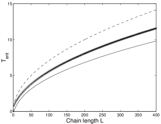
Figure 5: Scaling with chain-length $L$ of the time $T_{\mathrm{ent}}$ required to create a maximally entangled state between the ends. The points show numerical results obtained by saturating the rate equations (2a,2b). The solid and dashed curves show the analytic lower and upper bounds, $T_{\mathrm{ent}}\geq\sqrt{\lfloor L/2\rfloor/2}$ and $T_{\mathrm{ent}}\leq\sqrt{\lfloor L/2\rfloor}$ respectively.

We have loosened many an inequality during the proof of the square-root bound. Could the rate equations give a tighter bound? We can use essentially the same proof with the inequalities reversed to prove that a square-root bound is the best that can be obtained.

Instead of using $F_{k}(t)\leq 1$ to weaken the inequality right at the beginning, we use $F_{k}(t)\geq 1/2$, which is valid when the $F_{k}(t)$ saturate the inequalities in the rate equations, i.e. when $F_{k}(t)=f_{k}(t)$. Then, solutions of

$$\dot{l}_{k}(t)=\sqrt{2}\sqrt{l_{k-1}(t)-l_{k}(t)}$$

are lower bounds on $f_{k}(t)$. We can rescale the time $\tau=t/\sqrt{2}$ to so that the differential equation for $l_{k}(\tau)$ has the same form as that for $u_{k}(t)$ in the previous proof (Eq. 3). Assuming solutions of the form $l_{k}(\tau)=\tau^{2}/a_{k}$, solving the resulting recursion relation, and proving there is a lower bound on $f_{1}(t)$ of the appropriate form, leads to an upper bound on the scaling, for any evolution saturating the rate equations. For large chain lengths, the bound tends to $T_{\mathrm{ent}}\leq\sqrt{\lfloor L/2\rfloor}$ — also a square-root scaling. Therefore, the square-root bound we have derived is, up to a $\sqrt{2}$ numerical factor, the best that can be obtained from the entanglement rate equations (see Fig. 5).

How does our bound compare with the entanglement generation protocols described in the previous subsection? The generalized singlet fractions evolve quite differently in those protocols, compared to the evolution that would saturate the rate equations (compare Figs. 3 and 4 with Fig. 2). All existing protocols that we know of scale linearly with the length of the chain — no better than the trivial swapping protocol (entangle the middle qubits; move to the ends by swapping). It is an interesting open problem to determine whether any protocol can achieve a square-root scaling, or whether the bound derived via the rate equations is too weak and can not be saturated (which would suggest some improvement on the rate equations might be possible).

V Conclusions

We have investigated entanglement flow, both through individual particles and along networks of interacting particles. In both cases, we have derived differential equations relating the rate of entanglement generation to the existing entanglement in the system.

Entanglement flow through a particle is limited by the entanglement of that particle with the rest of the system, providing the system is in a pure state. (Previous work Cubitt et al. (2003) has already shown that the entanglement can be transmitted by a particle without that particles becoming entangled at all, if the system is in a mixed state.)

To describe entanglement flow along general networks of interacting particles, we have derived a set of entanglement rate equations, analogous to the rate equations for a chemical reaction. These can intuitively be interpreted as describing a flow of entanglement along the network. We have used the rate equations to prove a square-root lower bound on the scaling with system size of the time required to create a maximally entangled state, and compared this to existing entanglement generation protocols. Whether this bound is achievable, or whether the rate equations can be improved to give a tighter bound, remains an interesting open problem.

The entanglement rate equations were derived in the context of two-qubit entanglement creation. However, since they involve fidelity-based quantities, they can easily be extended to more general settings. Firstly, the quantities and equations can be extended to bipartite entanglement generation in arbitrary spaces, by taking fidelities with a bipartite maximally entangled state in the appropriate space. Secondly, they can be generalized to the multipartite setting, by taking fidelities with the desired multipartite entangled state (e.g. a GHZ state), rather than with a bipartite entangled state.

Together, the results establish a quantitative concept of entanglement flow in interacting systems. This is of interest as an abstract concept in itself, but could also be interesting both theoretically and practically: in the analysis of quantum algorithms, for example, since these often involve creating large amounts of entanglement during their operation. Or in physical implementations of quantum systems, in which it is important to carry out any manipulation (including entanglement creation) as fast as possible, to beat decoherence.

Appendix A Three-qubit chain

To derive the three-qubit result, we use a matrix analysis approach to calculating the concurrence, developed in Audenaert et al. (2001). Writing the Schmidt decomposition of the three-qubit system with respect to the partition $(b:ac)$ as $\mathinner{|\psi\rangle}_{abc}=\lambda_{1}\mathinner{|\varphi_{1}\rangle}_{ac}\mathinner{|\chi_{1}\rangle}_{b}+\lambda_{2}\mathinner{|\varphi_{2}\rangle}_{ac}\mathinner{|\chi_{2}\rangle}_{b}$, we can represent the state of $ab$ by a $4\times 2$ matrix $X=(\lambda_{1}\mathinner{|\varphi_{1}\rangle},\lambda_{2}\mathinner{|\varphi_{2}\rangle})$. The reduced density matrix is then given by $\rho_{ac}=XX^{\dagger}$.

The concurrence $C_{ac}$ of $\rho_{ac}$ can be obtained from the singular values of $A=X^{T}\Sigma X$, where $\Sigma=\sigma_{y}\otimes\sigma_{y}$ Audenaert et al. (2001). In our case, $A$ is a $2\times 2$ matrix (because $\rho_{ac}$ has rank two), with just two singular values: $\varsigma_{1}\geq\varsigma_{2}$. Thus $C_{ac}=\varsigma_{1}-\varsigma_{2}$. Since $\operatorname{tr}A^{\dagger}A=\varsigma_{1}^{2}+\varsigma_{2}^{2}$ and $|\det A|=\varsigma_{1}\varsigma_{2}$, we can also write this as

$$C_{ac}^{2}=\operatorname{tr}A^{\dagger}A-2|\det A|.$$ (5)

To calculate the time-derivative of the concurrence, we must calculate the derivatives of $\operatorname{tr}(A^{\dagger}A)$ and $|\det A|$. From its definition, $\dot{A}=\dot{X}^{T}\Sigma X+X^{T}\Sigma\,\dot{X}$. Meanwhile, $\mathrm{d}(\operatorname{tr}A^{\dagger}A)/\mathrm{d}t=\operatorname{tr}(A^{\dagger}\dot{A}+\dot{A}^{\dagger}A)$, which, after a little algebra, leads to

$$\frac{\mathrm{d}(\operatorname{tr}{A^{\dagger}A)}}{\mathrm{d}t}=4\operatorname{Re}\left(\operatorname{tr}\bigl{(}\Sigma\rho^{*}\Sigma\,\dot{X}X^{\dagger}\bigr{)}\right).$$ (6)

Since $A$ is a $2\times 2$ matrix, $\det A=\operatorname{tr}(A\sigma_{y}A^{T}\sigma_{y})/2$. Thus $\mathrm{d}(\det A)/\mathrm{d}t=\operatorname{tr}(\dot{A}\sigma_{y}A^{T}\sigma_{y}+A\sigma_{y}\dot{A}^{T}\sigma_{y})/2$ which, after a little more algebra, gives

$$\frac{\mathrm{d}(\det A)}{\mathrm{d}t}=4\operatorname{tr}\left(X\sigma_{y}X^{T}\Sigma X\sigma_{y}\dot{X}^{T}\Sigma\right).$$ (7)

The three-qubit chain evolves according to the Hamiltonian $H=H_{ab}\otimes\mathbbm{1}_{c}+\mathbbm{1}_{a}\otimes H_{bc}$. The two-qubit Hamiltonian $H_{ab}$ has a product decomposition $H_{ab}=\sum_{ij}a_{ij}\sigma_{i}\otimes\sigma_{j}$, where the Pauli matrices $\sigma_{i}$ are defined in the $\{\mathinner{|\chi_{1}\rangle},\mathinner{|\chi_{2}\rangle}\}$ basis, and coefficients $a_{ij}$ are real. Similarly for $H_{bc}$ and coefficients $c_{ij}$. The Schrödinger equation describing the evolution of the system state $\mathinner{|\psi\rangle}$ translates into an equation for the evolution of $X$:

$$\dot{X}=-i\sum_{ij}\left(a_{ij}\sigma_{i}\otimes\mathbbm{1}\,X\sigma_{j}^{T}+c_{ij}\mathbbm{1}\otimes\sigma_{i}\,X\sigma_{j}^{T}\right).$$

We can use this, along with expressions (6) and (7), in the time-derivative of (5) to obtain an expression for the derivative of the concurrence:

$$\frac{\mathrm{d}C_{ac}^{2}}{\mathrm{d}t}=h(H,\left|\psi\right>)\lambda_{1}\lambda_{2}.$$

The factor $h(H,\mathinner{|\psi\rangle})=\sum_{ij}a_{ij}h_{ij}^{a}+c_{ij}h_{ij}^{c}$ depends on both the interactions and the system state, and is a rather complicated sum over terms involving $a_{ij}$ and $c_{ij}$. We define

$$s_{ij}^{k} =\mathinner{\raisebox{-3.00003pt}{$\scriptstyle$}\langle\tilde{\varphi_{i}}|}\sigma_{k}\otimes\mathbbm{1}\mathinner{|\varphi_{j}\rangle}$$

$$t_{ij}^{k} =\mathinner{\raisebox{-3.00003pt}{$\scriptstyle$}\langle\tilde{\varphi_{i}}|}\mathbbm{1}\otimes\sigma_{k}\mathinner{|\varphi_{j}\rangle}$$

$$o_{ij} =\mathinner{\langle\varphi_{i}|\tilde{\varphi_{j}}\rangle}$$

$$h_{ix}^{a} =-i(\lambda_{1}^{2}s_{12}^{i}o_{11}+\lambda_{2}^{2}s_{21}^{i}o_{22})$$

$$h_{iy}^{a} =\lambda_{2}^{2}s_{21}^{i}o_{22}-\lambda_{1}^{2}s_{12}^{i}o_{11}$$

$$h_{iz}^{a} =-i\lambda_{1}\lambda_{2}(s_{21}^{i}o_{12}-s_{12}^{i}o_{21}),$$

and define $h_{ij}^{c}$ similarly to $h_{ij}^{a}$, but with the $s_{ij}$’s replaced by $t_{ij}$’s. Note that $s_{ii}^{k}=t_{ii}^{k}=0$. (The tildes denote the spin-flip operation Wootters (1998): $\mathinner{|\tilde{\varphi}\rangle}=\sigma_{y}\otimes\sigma_{y}\mathinner{|\varphi^{*}\rangle}$.) Then

$$h(H,\left|\psi\right>)=4\operatorname{Re}\Bigl{(}\sum_{ij}a_{ij}h_{ij}^{a}+c_{ij}h_{ij}^{c}\Bigr{)}+4\Bigl{\lvert}\sum_{ij}a_{ij}h_{ij}^{a}+c_{ij}h_{ij}^{c}\Bigr{\rvert}.$$

However, as we are primarily interested in the dependence on entanglement (i.e. the dependence on the Schmidt coefficients), we can bound the magnitudes of the $s_{ij}^{k}$, $t_{ij}^{k}$ and $o_{ij}$ by 1, and assume all terms sum in phase, giving the bound:

$$h(H,\left|\psi\right>)\leq\,8\sum_{ij}\left|a_{ij}\right|+\left|c_{ij}\right|,$$

which is independent of the system state, depending only on the interaction strengths.

Appendix B Entanglement rate equations

The proof of the entanglement rate equations revolves around Uhlmann’s theorem Uhlmann (1976); Jozsa (1994), which relates the fidelity of two mixed states to the fidelity of their purifications:

Theorem 1 (Uhlmann)

If $\rho$ and $\sigma$ are two states in the same Hilbert space $\mathcal{H}$, let $\mathinner{|\psi\rangle}$ and $\mathinner{|\varphi\rangle}$ be purifications of $\rho$ and $\sigma$ into a (in general larger) Hilbert space $\mathcal{H\otimes H^{\prime}}$. Then

$$F(\rho,\sigma)=\max_{\mathinner{|\psi\rangle},\mathinner{|\varphi\rangle}}\left|\left<\varphi|\psi\right>\right|^{2}$$

where the maximization is over all purifications.

Since any purification can be transformed into another by a unitary acting on $\mathcal{H^{\prime}}$, we can fix one of the purifications and only maximize over the other one. Also, global phases can be chosen to ensure the overlap $\mathinner{\langle\varphi|\psi\rangle}$ is real and positive, so the absolute value can be dropped.

Recall that the entanglement rate equations (2a,2b) involve two disjoint subsets, $A$ and $B$, of the entire set of particles $S$, which are interacting via two-particle interactions $H_{ij}$. We can apply Uhlmann’s theorem to the generalized singlet fraction of $\rho_{AB}$ at time $t$:

$$F_{AB}(t) =\max_{U_{A},U_{B}}\raisebox{-3.00003pt}{$\scriptstyle{}$}\left<\phi\right|\underbrace{\operatorname{tr}_{\!/\!ab}(U_{A}\otimes U_{B}\;\rho_{AB}(t)\;U_{A}^{\dagger}\otimes U_{B}^{\dagger})}_{\sigma_{ab}}\left|\phi\right>$$

$$=\max_{\begin{subarray}{c}U_{A},U_{B}\\ \mathinner{|\chi\rangle}\end{subarray}}\raisebox{-3.00003pt}{$\scriptstyle{}$}\left<\chi\right|U_{A}\otimes U_{B}\left|\psi\right>^{2}\quad\text{by Uhlmann}$$ (8)

$$=\raisebox{-3.00003pt}{$\scriptstyle{}$}\left<\bar{\chi}\right|\bar{U}_{A}\otimes\bar{U}_{A}\left|\psi\right>^{2},$$

where $\mathinner{|\bar{\chi}\rangle}$, $\bar{U}_{A}$ and $\bar{U}_{B}$ denote the particular state and unitaries achieving the maximum. (We are retaining the unitaries, rather than incorporating them into one of the purifications, for later convenience. Strictly speaking, they should be extended to $\mathcal{H}\otimes\mathcal{H^{\prime}}$ and written $U_{A}\otimes U_{B}\otimes\mathbbm{1}_{\mathrm{rest}}$. In the interests of economy, we will drop all $\mathbbm{1}_{\mathrm{rest}}$’s.)

The state $U_{A}\otimes U_{B}\mathinner{|\psi\rangle}$ can be chosen to be any fixed purification of the two-qubit density operator $\sigma_{ab}$. We use that freedom to make $\mathinner{|\psi\rangle}$ a purification of the overall system state $\rho_{S}$, which guarantees that $U_{A}\otimes U_{B}\mathinner{|\psi\rangle}$ is a purification of $\sigma_{ab}$, as required by Uhlmann’s theorem. As for $\mathinner{|\chi\rangle}$, since $\mathinner{|\phi\rangle}$ is already pure, it is simply an extension to $\mathcal{H}\otimes\mathcal{H^{\prime}}$: $\mathinner{|\chi\rangle}=\mathinner{|\phi\rangle}_{ab}\mathinner{|\vartheta\rangle}_{\mathrm{rest}}$ (the maximization then being over $\mathinner{|\vartheta\rangle}$).

If the system evolves under the Hamiltonian $H=\sum_{ij}H_{ij}$ for an infinitesimal time $\delta t$, the state evolves to $\rho_{AB}(t+\delta t)=\operatorname{tr}_{\!/\!AB}(e^{-iH\delta t}\rho_{S}(t)\,e^{iH\delta t})$. By writing the density matrix of the entire system, $\rho_{S}$, in a product basis for the partition $(AB:\mathrm{rest})$ and expanding the exponentials to first order in $\delta t$, it is straightforward to show that only interactions involving at least one particle in $AB$ give a first-order contribution to the evolution. Therefore, $H$ need only include that smaller set of interactions. Letting

$$U_{\delta t}=\exp\Bigl{(}-i\delta t\sum_{\mathchoice{\hbox to0.0pt{\hss$\displaystyle{\begin{subarray}{c}i\in S\\ j\in AB\end{subarray}}$\hss}}{\hbox to0.0pt{\hss$\textstyle{\begin{subarray}{c}i\in S\\ j\in AB\end{subarray}}$\hss}}{\hbox to0.0pt{\hss$\scriptstyle{\begin{subarray}{c}i\in S\\ j\in AB\end{subarray}}$\hss}}{\hbox to0.0pt{\hss$\scriptscriptstyle{\begin{subarray}{c}i\in S\\ j\in AB\end{subarray}}$\hss}}}H_{ij}\Bigr{)}$$

be the resulting (infinitesimal) unitary evolution operator, the singlet fraction after the evolution becomes

$$F_{AB}(t+\delta t)=\max_{\begin{subarray}{c}V_{A},V_{B}\\ \mathinner{|\zeta\rangle}\end{subarray}}\raisebox{-3.00003pt}{$\scriptstyle{}$}\left<\zeta\right|V_{A}\otimes V_{B}\cdot U_{\delta t}\left|\xi\right>^{2},$$ (9)

where we have used Uhlmann’s theorem again. The state $\mathinner{|\zeta\rangle}$ is again simply an extension of $\mathinner{|\phi\rangle}$ to $\mathcal{H}\otimes\mathcal{H^{\prime}}$, and $V_{A}\otimes V_{B}\,U_{\delta t}\mathinner{|\xi\rangle}$ can be chosen to be any fixed purification of the two-qubit density operator

$$\tau_{ab}=\operatorname{tr}_{\!/\!ab}\left(V_{A}\otimes V_{B}\,U_{\delta t}\rho_{S}\,U_{\delta t}^{\dagger}\,V_{A}^{\dagger}\otimes V_{B}^{\dagger}\right),$$

Again making use of this freedom, and recalling that we chose $\mathinner{|\psi\rangle}$ to be a purification of $\rho_{S}$, we can choose $\mathinner{|\xi\rangle}$ to be the same state as before: $\mathinner{|\xi\rangle}=\mathinner{|\psi\rangle}$.

The state $\mathinner{|\bar{\chi}\rangle}$ and unitaries $\bar{U}_{A}$ and $\bar{U}_{B}$ were defined to be those maximizing expression (8). Thus by definition,

$$\raisebox{-3.00003pt}{$\scriptstyle{}$}\left<\bar{\chi}\right|\bar{U}_{A}\otimes\bar{U}_{B}\left|\psi\right>\geq\raisebox{-3.00003pt}{$\scriptstyle{}$}\left<\chi\right|U_{A}\otimes U_{B}\left|\psi\right>$$

for all $\mathinner{|\chi\rangle}$, $U_{A}$ and $U_{B}$. In particular, this is true for infinitesimal changes, e.g. $\mathinner{|\bar{\chi}\rangle}+\delta t\mathinner{|\chi^{\bot}\rangle}$ where $\mathinner{|\chi^{\bot}\rangle}$ is orthogonal to $\mathinner{|\chi\rangle}$. Thus $\mathinner{\raisebox{-3.00003pt}{$\scriptstyle$}\langle\chi^{\bot}|}\bar{U}_{A}\otimes\bar{U}_{B}\mathinner{|\psi\rangle}\leq 0$. However, if this were strictly negative for some $\mathinner{|\chi^{\bot}\rangle}$, then $-\mathinner{|\chi^{\bot}\rangle}$ would make it positive. Therefore $\mathinner{\raisebox{-3.00003pt}{$\scriptstyle$}\langle\chi^{\bot}|}\bar{U}_{A}\otimes\bar{U}_{B}\mathinner{|\psi\rangle}=0$. Similarly, considering infinitesimal changes to the unitaries, we can show that:

$$\begin{gathered}\raisebox{-3.00003pt}{$\scriptstyle{}$}\left<\bar{\chi}\right|\bar{U}_{A}H_{A}\otimes\bar{U}_{B}\left|\psi\right>=0\quad\raisebox{-3.00003pt}{$\scriptstyle{}$}\left<\bar{\chi}\right|\bar{U}_{A}\otimes\bar{U}_{B}H_{B}\left|\psi\right>=0\\ \mathinner{\raisebox{-3.00003pt}{$\scriptstyle$}\langle\chi^{\bot}|}\bar{U}_{A}\otimes\bar{U}_{B}\mathinner{|\psi\rangle}=0.\end{gathered}$$ (12)

Expression (9) for the generalized singlet fraction at time $t+\delta t$ must tend to expression (8) (the corresponding expression for time $t$) as $\delta t\rightarrow 0$, so $\mathinner{|\zeta\rangle}=\mathinner{|\bar{\chi}\rangle}+\delta t\mathinner{|\chi^{\bot}\rangle}$ and $V_{A(B)}=\bar{U}_{A(B)}(\mathbbm{1}+i\delta tH_{A(B)})$, where $H_{A(B)}$ is a Hermitian operator on $A(B)$. Using this, expanding $U_{\delta t}=\mathbbm{1}-i\delta tH+O({\delta t^{2}})$ (where $H$ is the sum of interactions involving at least one particle in $A$ or $B$), and making use of relations (12), we have

$$F_{AB}(t+\delta t)=\raisebox{-3.00003pt}{$\scriptstyle{}$}\left<\bar{\chi}\right|\bar{U}_{A}\otimes\bar{U}_{B}(\mathbbm{1}-i\delta tH)\left|\psi\right>^{2}+O\left({\delta t^{2}}\right).$$

I.e. the state and unitaries maximizing expression (8) also maximize (9), to first order in $\delta t$.

Hamiltonian $H$ currently includes all interactions involving at least one particle in $A$ or $B$. By expanding $H$ in the previous expression as a sum over these two-particle interactions, we can use the same relations (12) to show that only interactions crossing the boundary of $A$ or $B$ need to be included to give the generalized singlet fraction to first order in $\delta t$:

$$F_{AB}(t+\delta t)=\raisebox{-3.00003pt}{$\scriptstyle{}$}\left<\bar{\chi}\right|\bar{U}_{A}\otimes\bar{U}_{B}\Bigl{(}\mathbbm{1}-i\delta t\sum_{\mathchoice{\hbox to0.0pt{\hss$\displaystyle{\begin{subarray}{c}i\notin A(B)\\ j\in A(B)\end{subarray}}$\hss}}{\hbox to0.0pt{\hss$\textstyle{\begin{subarray}{c}i\notin A(B)\\ j\in A(B)\end{subarray}}$\hss}}{\hbox to0.0pt{\hss$\scriptstyle{\begin{subarray}{c}i\notin A(B)\\ j\in A(B)\end{subarray}}$\hss}}{\hbox to0.0pt{\hss$\scriptscriptstyle{\begin{subarray}{c}i\notin A(B)\\ j\in A(B)\end{subarray}}$\hss}}}H_{ij}\Bigr{)}\left|\psi\right>^{2}+O\left({\delta t^{2}}\right).$$

Now, global phases were chosen to make it real and positive, so $\mathinner{\raisebox{-3.00003pt}{$\scriptstyle$}\langle\bar{\chi}|}\bar{U}_{A}\otimes\bar{U}_{B}\mathinner{|\psi\rangle}=\sqrt{F_{AB}(t)}$. Thus, expanding the square in the previous expression and only retaining first order terms in $\delta t$, we arrive at a first expression for the time-derivative of the generalized singlet fraction:

$$\dot{F}_{AB}(t)=\sqrt{F_{AB}(t)}\cdot\frac{1}{i}\sum_{\mathchoice{\hbox to0.0pt{$\displaystyle{\begin{subarray}{c}i\notin A(B)\\ j\in A(B)\end{subarray}}$\hss}}{\hbox to0.0pt{$\textstyle{\begin{subarray}{c}i\notin A(B)\\ j\in A(B)\end{subarray}}$\hss}}{\hbox to0.0pt{$\scriptstyle{\begin{subarray}{c}i\notin A(B)\\ j\in A(B)\end{subarray}}$\hss}}{\hbox to0.0pt{$\scriptscriptstyle{\begin{subarray}{c}i\notin A(B)\\ j\in A(B)\end{subarray}}$\hss}}}\raisebox{-3.00003pt}{$\scriptstyle{}$}\left<\varphi\right|H_{ij}\left|\psi\right>-\raisebox{-3.00003pt}{$\scriptstyle{}$}\left<\psi\right|H_{ij}\left|\varphi\right>$$ (13)

where $\mathinner{|\varphi\rangle}=\bar{U}_{A}^{\dagger}\otimes\bar{U}_{B}^{\dagger}\mathinner{|\bar{\chi}\rangle}$.

To proceed, we will need the following Proposition Bhatia (1997) which we use to prove the subsequent Lemma:

Proposition 2 (Fan-Hoffman)

For any operator $X$, the ordered singular values $\sigma^{\downarrow}_{i}$ of $X$ are individually greater than or equal to the ordered eigenvalues $r^{\downarrow}_{i}$ of $\operatorname{Re}X=(X+X^{\dagger})/2$. I.e. $\sigma^{\downarrow}_{i}\geq r^{\downarrow}_{i}$ $\forall i$.

Note that the eigenvalues of $\operatorname{Re}X$ can be negative, in which case the absolute values of the eigenvalues need not obey the Proposition.

Lemma 3

For any operator $X$, $(\operatorname{tr}|X|)^{2}-(\operatorname{tr}(\operatorname{Re}X))^{2}\geq\operatorname{tr}((\operatorname{Im}X)^{2})$, where $|X|=\sqrt{XX^{\dagger}}$, $\operatorname{Re}{X}=(X+X^{\dagger})/2$, and $\operatorname{Im}{X}=(X-X^{\dagger})/2i$.

Proof Assume initially that $\operatorname{tr}(\operatorname{Re}X)$ is non-negative. Defining $P$ ($N$) to be the set of positive (negative) eigenvalues of $\operatorname{Re}X$,

$$\sum_{i\neq j} \left(\sigma_{i}\sigma_{j}-r_{i}r_{j}\right)$$

$$= \sum_{i\neq j}\sigma_{i}\sigma_{j}-\sum_{\begin{subarray}{c}i,j\in P\\ i\neq j\end{subarray}}r_{i}r_{j}+\sum_{\begin{subarray}{c}i\in P\\ j\in N\end{subarray}}\left|r_{i}\right|\left|r_{j}\right|$$

$$+\sum_{\begin{subarray}{c}i\in N\\ j\in P\end{subarray}}\left|r_{i}\right|\left|r_{j}\right|-\sum_{\begin{subarray}{c}i,j\in N\\ i\neq j\end{subarray}}\left|r_{i}\right|\left|r_{j}\right|$$

$$= \sum_{\mathchoice{\hbox to0.0pt{\hss$\displaystyle{\begin{subarray}{c}i\,\text{or}\,j\notin P\\ i\neq j\end{subarray}}$\hss}}{\hbox to0.0pt{\hss$\textstyle{\begin{subarray}{c}i\,\text{or}\,j\notin P\\ i\neq j\end{subarray}}$\hss}}{\hbox to0.0pt{\hss$\scriptstyle{\begin{subarray}{c}i\,\text{or}\,j\notin P\\ i\neq j\end{subarray}}$\hss}}{\hbox to0.0pt{\hss$\scriptscriptstyle{\begin{subarray}{c}i\,\text{or}\,j\notin P\\ i\neq j\end{subarray}}$\hss}}}\sigma_{i}\sigma_{j}+\sum_{\begin{subarray}{c}i\in P\\ j\in N\end{subarray}}\left|r_{i}\right|\left|r_{j}\right|+\sum_{\begin{subarray}{c}i,j\in P\\ i\neq j\end{subarray}}\left(\sigma^{\downarrow}_{i}\sigma^{\downarrow}_{j}-r^{\downarrow}_{i}r^{\downarrow}_{j}\right)$$

$$+\sum_{i\in N}\left|r_{i}\right|\biggl{(}\sum_{j\in P}\left|r_{j}\right|-\sum_{\begin{subarray}{c}j\in N\\ j\neq i\end{subarray}}\left|r_{j}\right|\biggr{)}.$$

The first two terms are clearly positive, the third is positive by Proposition 2, and the last by the assumption that $\operatorname{tr}(\operatorname{Re}X)\geq 0$. Thus $\sum_{i\neq j}\left(\sigma_{i}\sigma_{j}-r_{i}r_{j}\right)\geq 0$. Now,

$$\bigl{(}\operatorname{tr} \left|X\right|\bigr{)}^{2}-\bigl{(}\operatorname{tr}(\operatorname{Re}X)\bigr{)}^{2}=\Bigl{(}\sum_{i}\sigma_{i}\Bigr{)}^{2}-\Bigl{(}\sum_{i}r_{i}\Bigr{)}^{2}$$

$$=\sum_{i}\sigma_{i}^{2}-\sum_{i}r_{i}^{2}+2\sum_{i\neq j}\left(\sigma_{i}\sigma_{j}-r_{i}r_{j}\right)$$

$$\geq\sum_{i}\sigma_{i}^{2}-\sum_{i}r_{i}^{2}\quad$$

$$=\operatorname{tr}\left(XX^{\dagger}\right)-\operatorname{tr}((\operatorname{Re}X)^{2})=\operatorname{tr}((\operatorname{Im}X)^{2})$$

where in the last line we have expanded $X=\operatorname{Re}X+i\operatorname{Im}X$, and used the fact that $\operatorname{Re}X$ and $\operatorname{Im}X$ are both Hermitian and that the trace of their commutator is 0.

For completeness, we can remove the assumption $\operatorname{tr}(\operatorname{Re}X)\geq 0$ by noting that, if there existed an operator $X$ with $\operatorname{tr}(\operatorname{Re}X)<0$ such that the Lemma did not hold, then the operator $-X$ would also violate the Lemma. But then $\operatorname{tr}(\operatorname{Re}(-X))\geq 0$, so the Lemma must hold for all operators. $\Box$

Recall that $H_{ij}$ really means $H_{ij}\otimes\mathbbm{1}_{\mathrm{rest}}$. Thus

$$\frac{1}{i}\bigl{(} \raisebox{-3.00003pt}{$\scriptstyle{}$}\left<\varphi\right|H_{ij}\left|\psi\right>-\mathrm{h.c.}\bigr{)}=\operatorname{tr}\Bigl{(}H_{ij}\cdot\frac{1}{i}\left(\operatorname{tr}_{\!/\!ij}\left|\psi\vphantom{\varphi}\right>\raisebox{-3.00003pt}{$\scriptstyle$}\left<\varphi\vphantom{\psi}\right|-\mathrm{h.c.}\right)\Bigr{)}$$

$$=2\operatorname{tr}\left(H_{ij}\operatorname{Im}X_{ij}\right)\quad\text{where }X_{ij}=\operatorname{tr}_{\!/\!ij}\left|\psi\vphantom{\varphi}\right>\raisebox{-3.00003pt}{$\scriptstyle$}\left<\varphi\vphantom{\psi}\right|$$

$$\leq 2\sqrt{\operatorname{tr}{H_{ij}^{2}}}\sqrt{\operatorname{tr}((\operatorname{Im}X_{ij})^{2})}\quad\text{by Cauchy-Schwartz}$$

$$\leq 2\left\|H_{ij}\right\|_{\mathrm{HS}}\sqrt{(\operatorname{tr}\left|X_{ij}\right|)^{2}-(\operatorname{tr}(\operatorname{Re}X_{ij}))^{2}}$$ (14)

using Lemma 3 in the last line. ($||\bullet||_{\mathrm{HS}}$ denotes the Hilbert-Schmidt norm.)

Finally, we need to relate the quantities under the square-root to generalized singlet fractions. Firstly, $(\operatorname{tr}(\operatorname{Re}X_{ij}))^{2}=(\operatorname{Re}(\operatorname{tr}\mathinner{|\psi\rangle\raisebox{-3.00003pt}{$\scriptstyle$}\langle\varphi|}))^{2}=\mathinner{\langle\varphi|\psi\rangle}^{2}=F_{AB}(t)$, since global phases were chosen to make $\mathinner{\langle\varphi|\psi\rangle}$ real and positive.

Secondly, $H_{ij}$ acts on one particle $j$ within $A$ or $B$, and a particle $i$ outside. If $j$ is in $A$, define the sets $A^{\prime}_{i}=A\cup i$ and $B^{\prime}_{i}=B$. If it is in $B$, define $A^{\prime}_{i}=A$, $B^{\prime}_{i}=B\cup i$. We apply Uhlmann’s theorem to the definition of the generalized singlet fraction for $\rho_{A^{\prime}_{i}B^{\prime}_{i}}$, and again choose the same state $\mathinner{|\psi\rangle}$ for one of the purifications. So long as $A^{\prime}_{i}$ and $B^{\prime}_{i}$ are disjoint, we have

$$F {}_{A^{\prime}_{i}B^{\prime}_{i}}(t)=\max_{\begin{subarray}{c}V_{A^{\prime}},V_{B^{\prime}}\\ \mathinner{|\zeta\rangle}\end{subarray}}\raisebox{-3.00003pt}{$\scriptstyle{}$}\left<\zeta\right|V_{A^{\prime}}\otimes V_{B^{\prime}}\left|\psi\right>^{2}$$

$$\geq\max_{V_{A^{\prime}},V_{B^{\prime}}}\raisebox{-3.00003pt}{$\scriptstyle{}$}\left<\bar{\chi}\right|\bar{U}_{A}V_{A^{\prime}}\otimes\bar{U}_{B}V_{B^{\prime}}\left|\psi\right>^{2}$$

$$=\max_{V_{A^{\prime}},V_{B^{\prime}}}\raisebox{-3.00003pt}{$\scriptstyle{}$}\left<\varphi\right|V_{A^{\prime}}\otimes V_{B^{\prime}}\left|\psi\right>^{2}\geq\max_{U_{ij}}\raisebox{-3.00003pt}{$\scriptstyle{}$}\left<\varphi\right|U_{ij}\left|\psi\right>^{2}$$

$$=\max_{U_{ij}}(\operatorname{tr}(U_{ij}X_{ij}))^{2}=\operatorname{tr}(\left|X_{ij}\right|)^{2},$$

where an inequality appears each time we restrict the maximization. The last line follows from the fact that, for any operator, $\operatorname{tr}|X|=\max_{U}|\operatorname{tr}(UX)|$, which is easily proved via the polar decomposition of $X$. If $A^{\prime}_{i}$ and $B^{\prime}_{i}$ have a particle in common (it must be particle $i$ if they do), then the second of the two inequalities is not valid. We can instead bound $\operatorname{tr}(|X_{ij}|)^{2}\leq 1$.

Thus, using $(\operatorname{tr}(\operatorname{Re}X_{ij}))^{2}=F_{AB}(t)$ and $\operatorname{tr}(\left|X_{ij}\right|)^{2}\leq F_{A^{\prime}_{i}B^{\prime}_{i}}(t)$ ($A^{\prime}_{i}$ and $B^{\prime}_{i}$ disjoint) or $\operatorname{tr}(\left|X_{ij}\right|)^{2}\leq 1$ ($A^{\prime}_{i}$ and $B^{\prime}_{i}$ overlapping) in (14), and substituting the result in (13), we arrive at a version of the entanglement rate equation:

$$\dot{F}_{AB}(t)\leq 2\sum_{\mathchoice{\hbox to0.0pt{$\displaystyle{\begin{subarray}{c}i\notin A(B)\\ j\in A(B)\end{subarray}}$\hss}}{\hbox to0.0pt{$\textstyle{\begin{subarray}{c}i\notin A(B)\\ j\in A(B)\end{subarray}}$\hss}}{\hbox to0.0pt{$\scriptstyle{\begin{subarray}{c}i\notin A(B)\\ j\in A(B)\end{subarray}}$\hss}}{\hbox to0.0pt{$\scriptscriptstyle{\begin{subarray}{c}i\notin A(B)\\ j\in A(B)\end{subarray}}$\hss}}}\left\|H_{ij}\right\|_{\mathrm{HS}}\sqrt{F_{AB}(t)\vphantom{F_{A^{\prime}_{i}}}}\sqrt{F_{A^{\prime}_{i}B^{\prime}_{i}}(t)-F_{AB}(t)},$$

where $F_{A^{\prime}_{i}B^{\prime}_{i}}$ is defined to be $1$ if $A^{\prime}_{i}$ and $B^{\prime}_{i}$ overlap.

To describe entanglement flow in a network of interacting particles, one such rate equation must be written down for all meaningful generalized singlet fractions that can be defined on the network (‘meaningful’ implying that the sets $A$ and $B$ include particles $a$ and $b$ respectively, and are each be made up of ‘one piece’).

Recall that, since $A^{\prime}_{i}$ and $B^{\prime}_{i}$ are subsets of $A^{\prime}$ and $B^{\prime}$ (see Fig. 1), $F_{A^{\prime}_{i}B^{\prime}_{i}}\leq F_{A^{\prime}B^{\prime}}$. We can use this to arrive at the simpler version of the entanglement rate equations presented in the main text:

$$\dot{F}_{AB}(t)\leq 2\sum_{\mathchoice{\hbox to0.0pt{\hss$\displaystyle{\begin{subarray}{c}i\notin A(B)\\ j\in A(B)\end{subarray}}$\hss}}{\hbox to0.0pt{\hss$\textstyle{\begin{subarray}{c}i\notin A(B)\\ j\in A(B)\end{subarray}}$\hss}}{\hbox to0.0pt{\hss$\scriptstyle{\begin{subarray}{c}i\notin A(B)\\ j\in A(B)\end{subarray}}$\hss}}{\hbox to0.0pt{\hss$\scriptscriptstyle{\begin{subarray}{c}i\notin A(B)\\ j\in A(B)\end{subarray}}$\hss}}}\left\|H_{ij}\right\|_{\mathrm{HS}}\sqrt{F_{AB}(t)}\sqrt{F_{A^{\prime}B^{\prime}}(t)-F_{AB}(t)}.$$

Appendix C General tripartite chains

The first half of the derivation of the entanglement rate equations given in Appendix B can be re-used in the proof of the tripartite chain result. Recall that the three systems $A$, $B$ and $C$ making up the chain are in an overall pure state $\mathinner{|\psi\rangle}_{ABC}$, and interact by nearest-neighbour interactions: $H=H_{AB}+H_{BC}$. As noted in subsection III.1, the entangled fraction $F_{AC}$ of $\rho_{AC}$ can be expressed as a maximization over unitaries $U_{A}$ and $U_{C}$ rather than states. Applying Uhlmann’s relation, it can be rewritten

$$F_{AC}=\max_{\begin{subarray}{c}U_{A},U_{C}\\ \mathinner{|\chi\rangle}\end{subarray}}\raisebox{-3.00003pt}{$\scriptstyle{}$}\left<\chi\right|U_{A}\otimes U_{C}\left|\psi\right>=\left<\varphi|\psi\right>.$$

We can choose $\mathinner{|\psi\rangle}$ to be the overall system state $\mathinner{|\psi\rangle}_{ABC}$, since this is a purification of $\rho_{AC}$. $\mathinner{|\chi\rangle}$ is then an extension of a maximally entangled state $\mathinner{|\phi\rangle}_{AC}$ on $\mathcal{H}_{AC}$ to the space $\mathcal{H}_{ABC}$: $\mathinner{|\chi\rangle}=\mathinner{|\phi\rangle}_{AC}\mathinner{|\zeta\rangle}_{B}$. We define $\mathinner{|\varphi\rangle}=\bar{U}_{A}^{\dagger}\otimes\bar{U}_{C}^{\dagger}\mathinner{|\bar{\chi}\rangle}=\mathinner{|\bar{\phi}\rangle}_{AC}\mathinner{|\bar{\zeta}\rangle}$, where bars denote the particular unitaries and states achieving the maximum.

Although the rate equations involve the generalized singlet fraction, up to expression (13) the derivation in Appendix B applies equally well to the entangled fraction. Expression (13) then becomes

$$\dot{F}_{AC}(t)=\sqrt{F_{AC}(t)}\cdot\frac{1}{i}\left(\raisebox{-3.00003pt}{$\scriptstyle{}$}\left<\varphi\right|H\left|\psi\right>-\raisebox{-3.00003pt}{$\scriptstyle{}$}\left<\psi\right|H\left|\varphi\right>\right),$$ (15)

Now, writing the state in its Schmidt decomposition for the partition $(B:AC)$, $\mathinner{|\psi\rangle}_{ABC}=\sum_{i}\lambda_{i}\mathinner{|\psi_{i}\rangle}_{AC}\mathinner{|i\rangle}_{B}$, where we sort the Schmidt coefficients in descending order: $\lambda_{1}\geq\lambda_{2}\geq\dots\geq\lambda_{n}$. Extending $\{\mathinner{|i\rangle}_{B}\}$ to form a complete basis for $\mathcal{H}_{B}$, $\mathinner{|\varphi\rangle}$ can be written in the product decomposition $\mathinner{|\varphi\rangle}=\mathinner{|\bar{\phi}\rangle}_{AC}\sum_{i}\alpha_{i}\mathinner{|i\rangle}_{B}$ (the $\alpha_{i}$ are complex in general).

We know that $\mathinner{|\varphi\rangle}$ maximizes $\mathinner{\langle\varphi|\psi\rangle}=\sum_{i}\alpha_{i}^{*}\lambda_{i}\left<\bar{\phi}|\psi_{i}\right>$. Clearly, the phases of $\alpha_{i}$ must be chosen to cancel the phases of $\mathinner{\langle\bar{\phi}|\psi_{i}\rangle}$. The relationship between the magnitudes of the $\alpha_{i}$’s and $\mathinner{\langle\bar{\phi}|\psi_{i}\rangle}$’s can be found using Lagrange multipliers, with the normalization constraint $\sum_{i}|\alpha_{i}|^{2}=1$, yielding

$$\alpha_{i}=\frac{\lambda_{i}\left<\psi_{i}|\bar{\phi}\right>}{\sqrt{\sum_{k}\lambda_{k}^{2}\left|\left<\bar{\phi}|\psi_{k}\right>\right|^{2}}}$$ (16)

We also know that, for any Hamiltonian acting only on $A$ or $C$, $\mathinner{\raisebox{-3.00003pt}{$\scriptstyle$}\langle\varphi|}H_{A}\mathinner{|\psi\rangle}=\mathinner{\raisebox{-3.00003pt}{$\scriptstyle$}\langle\varphi|}H_{C}\mathinner{|\psi\rangle}=0$ (applying the same reasoning as used to prove relations (12) in Appendix B). Thus

$$\alpha_{1}^{*}\lambda_{1}\raisebox{-3.00003pt}{$\scriptstyle{}$}\left<\bar{\phi}\right|H_{A(C)}\left|\psi_{i}\right>=-\sum_{i\neq 1}\alpha_{i}^{*}\lambda_{i}\raisebox{-3.00003pt}{$\scriptstyle{}$}\left<\bar{\phi}\right|H_{A(C)}\left|\psi_{i}\right>.$$ (17)

Now, the system Hamiltonian $H=H_{AB}+H_{AC}$. $\raisebox{-3.00003pt}{$\scriptstyle{}$}\left<\varphi\right|H_{AB}\left|\psi\right>=\sum_{ij}\alpha_{i}^{*}\lambda_{j}\mathinner{\raisebox{-3.00003pt}{$\scriptstyle$}\langle\bar{\phi}|}\mathinner{\raisebox{-3.00003pt}{$\scriptstyle B$}\langle i|}H_{AB}\mathinner{|j\rangle}_{B}\mathinner{|\psi_{j}\rangle}$. For the $i=j=1$ terms in the sum, $\mathinner{\raisebox{-3.00003pt}{$\scriptstyle B$}\langle 1|}H_{AB}\mathinner{|1\rangle}_{B}$ is just some Hamiltonian acting only on $A$. Similarly for $\mathinner{\raisebox{-3.00003pt}{$\scriptstyle B$}\langle 1|}H_{BC}\mathinner{|1\rangle}_{B}$. Thus using (16) and (17),

$$\raisebox{-3.00003pt}{$\scriptstyle{}$}\left<\varphi\right|H\left|\psi\right>= \sum_{i\neq 1}\alpha_{i}^{*}\lambda_{i}\bigl{(}\raisebox{-3.00003pt}{$\scriptstyle{}$}\left<\bar{\phi},i\right|H\left|\psi_{i},i\right>-\raisebox{-3.00003pt}{$\scriptstyle{}$}\left<\bar{\phi},1\right|H\left|\psi_{i},1\right>\bigr{)}$$

$$+\sum_{i\neq j}\alpha_{i}^{*}\lambda_{i}\raisebox{-3.00003pt}{$\scriptstyle{}$}\left<\bar{\phi},i\right|H\left|\psi_{j},j\right>$$

$$= \sum_{i\neq 1}\lambda_{i}^{2}h_{ii}+\sum_{i\neq j}\lambda_{i}\lambda_{j}h_{ij},$$

where

$$h_{ii} =\frac{\left<\psi_{i}|\bar{\phi}\right>\bigl{(}\raisebox{-3.00003pt}{$\scriptstyle{}$}\left<\bar{\phi},i\right|H\left|\psi_{i},i\right>-\raisebox{-3.00003pt}{$\scriptstyle{}$}\left<\bar{\phi},1\right|H\left|\psi_{i},1\right>\bigr{)}}{\sqrt{\sum_{k}\lambda_{k}^{2}\left|\left<\bar{\phi}|\psi_{k}\right>\right|^{2}}}$$

$$h_{ij} =\frac{\left<\psi_{i}|\bar{\phi}\right>\raisebox{-3.00003pt}{$\scriptstyle{}$}\left<\bar{\phi},i\right|H\left|\psi_{i},j\right>}{\sqrt{\sum_{k}\lambda_{k}^{2}\left|\left<\bar{\phi}|\psi_{k}\right>\right|^{2}}}\quad\text{for }i\neq j.$$

Using this in (15), and bounding $(h_{ij}-h_{ij}^{*})/i\leq 2|H|=2(|H_{AB}|_{\infty}+|H_{BC}|_{\infty})$ (where $|M|_{\infty}=\max_{ij}|M_{ij}|$ denotes the $l_{\infty}$ norm), we arrive at the final result:

$$\dot{F}_{AC}(t)\leq 2\left|H\right|\sqrt{F_{AC}(t)}\,\Bigl{(}\sum_{ij}\lambda_{i}\lambda_{j}-\lambda_{1}^{2}\Bigr{)}.$$

References

- Schumacher (1995) B. Schumacher, Phys. Rev. A. 51, 2738 (1995).
- QIC (2001) Quantum Inf. Comput. 1, No. 1 (2001).
- Nielsen (1999) M. A. Nielsen, Phys. Rev. Lett. 83, 436 (1999).
- Bennett et al. (1993) C. H. Bennett et al., Phys. Rev. Lett. 70, 1895 (1993).
- Dür et al. (2001) W. Dür et al., Phys. Rev. Lett. 87, 137901 (2001).
- Bennett et al. (2003) C. H. Bennett et al., IEEE Trans. Inf. Theory 49, 1895 (2003).
- Childs et al. (2003) A. M. Childs et al., Quantum Inf. Comput. 3, 97 (2003).
- Khaneja et al. (2001) N. Khaneja, R. Brockett, and S. J. Glaser, Phys. Rev. A. 63, 032308 (2001).
- Bremner et al. (2004) M. J. Bremner et al., Phys. Rev. A. 69, 012313 (2004).
- Vidal et al. (2002) G. Vidal, K. Hammerer, and J. I. Cirac, Phys. Rev. Lett. 88, 237902 (2002).
- Zanardi et al. (2000) P. Zanardi, C. Zalka, and L. Faoro, Phys. Rev. A. 62, 030301(R) (2000).
- Cubitt et al. (2003) T. S. Cubitt et al., Phys. Rev. Lett. 91, 037902 (2003).
- Wootters (1998) W. K. Wootters, Phys. Rev. Lett. 80, 2245 (1998).
- Bennett et al. (1996) C. H. Bennett et al., Phys. Rev. A. 54, 3824 (1996).
- Audenaert et al. (2001) K. Audenaert et al., Phys. Rev. A. 64, 052304 (2001).
- Jozsa (1994) R. Jozsa, J. Mod. Opt. 41 (1994).
- Horodecki et al. (1999) M. Horodecki, P. Horodecki, and R. Horodecki, Phys. Rev. A. 60, 1888 (1999).
- Verstraete and Verschelde (2002) F. Verstraete and H. Verschelde, Phys. Rev. A. 66, 022307 (2002).
- not (a) According to the definition given, the generalized singlet fraction is only defined for spaces in which qubits can be embedded. It can be extended to general spaces if, instead of embedding a qubit, we embed a qudit of appropriate dimension. It can also be extended to measure multi-partite entanglement by replacing the bipartite maximally entangled state with the desired multipartite entangled state (e.g. a GHZ state).
- Farhi and Gutmann (1998) E. Farhi and S. Gutmann, Phys. Rev. A. 58, 915 (1998).
- Ambainis (2002) A. Ambainis, J. Comput. Syst. Sci. 64, 750 (2002).
- Briegel and Raussendorf (1002) H. J. Briegel and R. Raussendorf, Phys. Rev. Lett. 86, 910 (1002).
- Verstraete et al. (2004) F. Verstraete, M. Popp, and J. I. Cirac, Phys. Rev. Lett. 92, 027901 (2004).
- Nielsen et al. (2002) M. A. Nielsen et al., Phys. Rev. A. 66, 022317 (2002).
- Wocjan et al. (2002) P. Wocjan et al., Quantum Inf. Comput. 2, 133 (2002).
- Khaneja and Glaser (2002) N. Khaneja and S. J. Glaser, Phys. Rev. A. 66, 060301(R) (2002).
- Christandl et al. (2003) M. Christandl et al., quant-ph/0309131 (2003).
- Yung et al. (2003) M.-H. Yung, D. W. Leung, and S. Bose, quant-ph/0312105 (2003).
- not (b) Ref. Christandl et al. (2003) states that the time required to entangle the end qubits is independent of the length of the chain. For this to be the case, the interaction strengths must be increased for longer chains. If the interaction strengths are normalized, the scaling is linear.
- Osborne and Linden (2003) T. J. Osborne and N. Linden, quant-ph/0312141 (2003).
- Uhlmann (1976) A. Uhlmann, Rep. Math. Phys. 9 (1976).
- Bhatia (1997) R. Bhatia, Matrix Analysis, Graduate Texts in Mathematics (Springer, 1997).
- Nielsen and Chuang (2000) M. A. Nielsen and I. L. Chuang, Quantum Computation and Quantum Information (Cambridge University Press, 2000).