Large geometric phases and non-elementary monopoles

Abstract

Degeneracies in the spectrum of an adiabatically transported quantum system are important to determine the geometrical phase factor, and may be interpreted as magnetic monopoles. We investigate the mechanism by which constraints acting on the system, related to local symmetries, can create arbitrarily large monopole charges. These charges are associated with different geometries of the degeneracy. An explicit method to compute the charge as well as several illustrating examples are given.

PACS : 03.65.Vf Phases: geometric; dynamic or topological

1 Introduction

When a quantum system is adiabatically transported along a closed loop $\mathcal{L}$ in a parameter space, in addition to the usual dynamical phase every non-degenerate eigenstate accumulates an extra phase $\Delta\Phi$. For a 3d-parameter space, M. V. Berry gives a geometrical interpretation of $\Delta\Phi$ as the flux of a magnetic-like field $\mathbf{B}$ through a surface with boundary $\mathcal{L}$ [Berry84a]. The degeneracies of the spectrum in parameter space are the singularities of the vector field $\mathbf{B}$, and therefore play an important role in connexion with the geometric phase. Each degeneracy can be seen as a charge distribution located at the contact point between energy surfaces. Because the eigenstates are smooth and single valued outside the degeneracies, the total charge of the distribution, i.e. the monopole charge or moment, is necessarily an integer multiple of the elementary charge $g_{0}=1/2$. In the generic case of a diabolical contact [Berry84a], the monopole charges are precisely $\pm g_{0}$. However, higher integer multiples of $g_{0}$ may occur. For instance, for light propagating through a twisted anisotropic dielectric medium there are experimental situations [Berry86a] where the monopole charges are $\pm 2g_{0}$. Other examples arise in condensed matter physics. In a bidimensional periodic crystalline lattice, the Hall conductance of a gas of independent electrons is proportional to a topological index, the Chern index, that measures the net charge inside a closed surface associated to the first Brillouin zone [Simon83a]. In some models, large jumps of the Chern index that cannot be explained by elementary charges have been observed [Leboeuf+90a] [Faure/Leboeuf93a].

Our purpose is to discuss a generic mechanism for the production of monopole charges larger than $g_{0}$. The mechanism is due to constraints that act on the system, and may be associated to local symmetries. Section 2 introduces the notation and some general formulae for $\Delta\Phi$. The generic case of a diabolical contact is briefly recalled in section 3. In section 4, which is the central part of the paper, a broader class of situations that incorporates constraints is considered. The consequences on the geometry of the contact point and on the corresponding monopole charges are discussed, and a method to explicitly compute them is introduced. The latter provides an alternative and simple view of the quantization of the monopole charge as a sum over winding numbers associated to Dirac strings. We illustrate the general approach by two examples in section 5, and show how arbitrarily large multiples of $g_{0}$ can actually be generated in 6. The last section contains a discussion of some of the results obtained.

2 Background material

We consider a quantum system governed by a Hamiltonian depending on three real parameters $\mathbf{r}=(x,y,z)$. We denote $\mathcal{P}$ the parameter space and suppose that in the neighborhood of $\mathbf{r}=\mathbf{0}$ two eigenvalues are close to each other. Hence, the coupling to other states can be neglected and the Hamiltonian can be restricted to a bidimensional eigenspace. The most general form of the reduced Hamiltonian is

$$H(\mathbf{r})\ =\ \begin{pmatrix}s(\mathbf{r})+e_{z}(\mathbf{r})&e_{x}(\mathbf{r})-\mathrm{i}\,e_{y}(\mathbf{r})\\[12.91663pt] e_{x}(\mathbf{r})+\mathrm{i}\,e_{y}(\mathbf{r})&s(\mathbf{r})-e_{z}(\mathbf{r})\end{pmatrix}\ =\ s(\mathbf{r})+\text{e}(\mathbf{r}).\boldsymbol{\sigma}$$ (1)

$s(\mathbf{r})$ and the three components of $\text{e}(\mathbf{r})=[e_{x}(\mathbf{r}),e_{y}(\mathbf{r}),e_{z}(\mathbf{r})]$ are smooth real functions in $\mathcal{P}$. $\boldsymbol{\sigma}=[\sigma_{x},\sigma_{y},\sigma_{z}]$ are the Pauli matrices.

The eigenvalues of $H(\mathbf{r})$ are given by

$$E_{\pm}(\mathbf{r})\ =\ s(\mathbf{r})\pm e(\mathbf{r})$$ (2)

where $e=\sqrt{e_{x}^{2}+e_{y}^{2}+e_{z}^{2}}$. The points $\mathbf{r}$ of the parameter space where degeneracies occur are given by the set $\mathcal{M}$ where $e$ vanishes.

One possible orthonormal eigenbasis corresponding to $E_{\pm}(\mathbf{r})$ is

$$|\psi_{\pm}(\mathbf{r})\rangle\ \stackrel{{\scriptstyle\mbox{\rm\scriptsize def}}}{{=}}\ \frac{1}{\sqrt{2e(\mathbf{r})\,\bigl{(}e(\mathbf{r})\mp e_{z}(\mathbf{r})\bigr{)}}}\begin{pmatrix}e_{x}(\mathbf{r})-\mathrm{i}\,e_{y}(\mathbf{r})\\[4.30554pt] \pm e(\mathbf{r})-e_{z}(\mathbf{r})\end{pmatrix}\;.$$ (3)

It follows from this expression that the eigenstates of $H$ are not only singular on $\mathcal{M}$ but more generally on a larger subset $\mathcal{D}$ of $\mathcal{P}$. With the choice (3), $\mathcal{D}$ is given by the points where $e(\mathbf{r})\mp e_{z}(\mathbf{r})$ vanishes. For convenience, we split $\mathcal{D}$ into two sets, $\mathcal{D}_{+}$ and $\mathcal{D}_{-}$, that corresponds to $e_{x}(\mathbf{r})=e_{y}(\mathbf{r})=0$ and $e_{z}(\mathbf{r})\geq 0$ ($e_{z}(\mathbf{r})\leq 0$), respectively. These two sets intersect on $\mathcal{M}$.

Let $\mathcal{L}$ be any closed loop in $\mathcal{P}$ not intersecting $\mathcal{D}$. Berry [Berry84a] gave a geometrical interpretation (that is, coordinate free in $\mathcal{P}$) of the non-dynamical part $\Delta\Phi_{\pm}$ of the phase shift that $|\psi_{\pm}(\mathbf{r})\rangle$ acquires when $H(\mathbf{r})$ follows $\mathcal{L}$ adiabatically. Simon [Simon83a] completed the picture with a topological interpretation of Berry’s phase in terms of connection on a suitable fiber bundle. Topological arguments were anticipated in [Stone76a, see in particular the section:“A topological test for intersections”, p.85]. The phase shift after one traversal of $\mathcal{L}$ is given by the circulation

$$\Delta\Phi_{+}=-\Delta\Phi_{-}=\Delta\Phi\ \stackrel{{\scriptstyle\mbox{\rm\scriptsize def}}}{{=}}\ \oint_{\mathcal{L}}\mathbf{A}(\mathbf{r}).\,d\mathbf{l}$$ (4)

of the vector $\mathbf{A}\stackrel{{\scriptstyle\mbox{\rm\scriptsize def}}}{{=}}-\mathrm{Im}\Bigl{[}\langle\psi_{+}|\boldsymbol{\nabla_{\!r}}|\psi_{+}\rangle\Bigr{]}.$ By Stokes’s theorem, $\Delta\Phi$ can alternatively be computed from,

$$\Delta\Phi=\int_{\mathcal{S}}\mathbf{B}(\mathbf{r}).\,d\boldsymbol{\Sigma}\;.$$ (5)

$\mathcal{S}$ is any surface in $\mathcal{P}$ not intersecting $\mathcal{D}$ whose border is $\mathcal{L}$. $\mathbf{B}(\mathbf{r})$ is the 3-vector field (more generally a 2-form) obtained by taking the curl of $\mathbf{A}$. Specifically, outside $\mathcal{D}$ and in the two–dimensional subspace where our analysis is restricted

$$\mathbf{B}=\frac{\langle\psi_{+}|\boldsymbol{\nabla_{\!r}}\,H|\psi_{-}\rangle\wedge\langle\psi_{-}|\boldsymbol{\nabla_{\!r}}\,H|\psi_{+}\rangle}{(E_{+}-E_{-})^{2}}\;.$$ (6)

From (1), (2) and (3) we may write, outside $\mathcal{D}$,

$$\mathbf{A}=\frac{e_{y}\boldsymbol{\nabla_{\!r}}\,e_{x}-e_{x}\boldsymbol{\nabla_{\!r}}\,e_{y}}{2(e_{x}^{2}+e_{y}^{2})}\left(1+\frac{e_{z}}{e}\right)\;,$$ (7)

and

$$\mathbf{B}=\frac{1}{2e^{3}}\Bigl{[}e_{x}(\boldsymbol{\nabla_{\!r}}\,e_{y}\wedge\boldsymbol{\nabla_{\!r}}\,e_{z})+e_{y}(\boldsymbol{\nabla_{\!r}}\,e_{z}\wedge\boldsymbol{\nabla_{\!r}}\,e_{x})+e_{z}(\boldsymbol{\nabla_{\!r}}\,e_{x}\wedge\boldsymbol{\nabla_{\!r}}\,e_{y})\Bigr{]}\;.$$ (8)

3 Generic case (no constraints)

Generically $\mathcal{M}$ is either empty or an isolated point (see [vonNeumann/Wigner29a]). We consider the latter case and work in a local chart centered at the contact point, that we assume is located at $\mathbf{r}=\mathbf{0}$. Since generically

$$\Lambda\ \stackrel{{\scriptstyle\mbox{\rm\scriptsize def}}}{{=}}\ \det\bigl{[}\boldsymbol{\nabla_{\!r}}\,e_{x},\boldsymbol{\nabla_{\!r}}\,e_{y},\boldsymbol{\nabla_{\!r}}\,e_{z}\bigr{]}_{\left|\mathbf{r}=\mathbf{0}\right.}$$ (9)

is different from zero, by virtue of the local inversion theorem we can consider $(e_{x},e_{y},e_{z})$ to be a new local chart in a neighborhood of $\mathbf{r}=\mathbf{0}$. In other words, we can take $\mathbf{r}=\text{e}$. This is the generic case. The two energy surfaces $E_{\pm}(\mathbf{r})$ intersect through an isolated doubly-conical contact point (diabolical point) [vonNeumann/Wigner29a]. From (8) we have

$$\mathbf{B}(\mathbf{r})=\frac{\mathbf{r}}{2||\mathbf{r}||^{3}}\ .$$ (10)

Close to a conical intersection the vector $\mathbf{B}$ corresponds therefore to the field created by a magnetic monopole of charge $g=g_{0}=1/2$ [Dirac31a, Dirac78a] (for the state $|\psi_{-}(\mathbf{r})\rangle$ the opposite charge must be taken). $\mathbf{A}(\mathbf{r})$ is the vector potential associated to it. The sets $\mathcal{D}_{\pm}$ are the well known Dirac (half) strings which physically can be interpreted as semi-infinite solenoids (with end points at $\mathbf{r}=\mathbf{0}$) carrying a magnetic flux $\pm 4\pi g_{0}$, respectively. This magnetic analogy cannot however be extended globally since there is no superposition theorem available here.

4 Finite number of constraints

4.1 Non-elementary monopoles

We now consider situations where some constraints acting on the system are present. These constraints can be thought of as independent real control parameters $\lambda=\{\lambda_{n}\}_{n\in\{0,\ldots,C-1\}}$ that impose $C$ independent relations between the derivatives of e at $\mathbf{r}=\mathbf{0}$. Physically the control parameters are distinct from the adiabatic parameters $\mathbf{r}$ in that they reflect a local symmetry in $\mathcal{P}$ and therefore do not change during the adiabatic transport along $\mathcal{L}$. Due to these additional constraints, it may happen that the determinant $\Lambda$ defined by Eq. (9) vanishes. The latter condition requires generically the existence of one external parameter $\lambda$ in addition to $\mathbf{r}$. In that case, the contact between the energy surfaces restricted to the $\mathbf{r}$-space $\mathcal{P}$ is not a diabolical point anymore (see figure 1). For instance, the charge $g=2g_{0}$ occasionally observed in Ref. [Leboeuf+90a] was found to correspond to a parabolic contact. By increasing the number of parameters $\lambda$ one can accordingly cancel an increasing number of derivatives of e at $\mathbf{r}=\mathbf{0}$, and therefore increase accordingly the degree of tangency of the surfaces defined by (2).

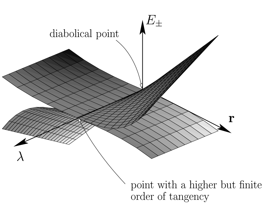
Figure 1: The unfolding shown in this picture illustrates the changes in the geometry of the contact point between two energy surfaces induced by the variation of some control parameter $\lambda$.

If the number of constraints $C$ is finite, in the full $(C+3)$–dimensional parameter space (that includes both the adiabatic and the control parameters), the set of degeneracies is $C$-dimensional and generically crosses transversely at an isolated point located at $\mathbf{r}=\mathbf{0}$ any 3-dimensional space defined by $\lambda=\mathrm{constant}$. It requires an infinite number of constraints to transform $\mathcal{M}$ into a continuous family of points since an infinite number of vanishing derivatives of e is needed. This is the situation when, for instance, the system is invariant under a global symmetry, like the time reversal symmetry. In that case $e_{y}\equiv 0$ at any point in $\mathcal{P}$ and $\mathcal{M}$ is a 1-dimensional sub-manifold of $\mathcal{P}$. Global symmetries that increase the dimension of the contact manifold are not considered here, we restrict to the cases where the number of constraints due to local symmetries is finite.

Under these assumptions, it follows from (8) that $\mathrm{div}\,\mathbf{B}$ is a distribution with support in $\mathbf{r}=\mathbf{0}$. It can therefore be expanded as,

$$\mathrm{div}\,\mathbf{B}=g\,\delta(\mathbf{r})+\text{terms involving derivatives of~{}$\delta(\mathbf{r})$.}$$ (11)

As for an arbitrary circuit in parameter space [Berry84a, p. 55], and in contrast to the diabolical contact, generically in the two–dimensional subspace of the degeneracy the geometric phase is not completely determined by (11) because of the non-vanishing curl of (8). Our purpose is to determine an explicit rule to compute $g$. A more detailed qualitative discussion of the contribution to the geometric phase of the curl of $\mathbf{B}$ and of the additional multipolar terms in (11) will be made in the final section.

4.2 The monopole charge as a sum of winding numbers

One of the most remarkable properties of the monopoles is the quantization of their charge, which can only take integer multiple values of $g_{0}=1/2$. This easily follows from a topological argument given by [Stone76a]. Consider a small loop $\mathcal{L}$ that is smoothly retracted to a point without crossing $\mathcal{D}$. Because the eigenstates remain smooth and single valued, $\Delta\Phi$ must tend to an integer multiple of $2\pi$. But $\Delta\Phi$ is the flux of $\mathbf{B}$ through any surface $\mathcal{S}$ with boundary $\mathcal{L}$. When $\mathcal{L}$ shrinks to a point, $\mathcal{S}$ tends either to a point or to a closed finite surface that possibly encloses a monopole charge $g$. Therefore $\Delta\Phi\to 4\pi g$, which must be an integer multiple of $2\pi$. The quantization of $g$ follows.

This argument is, however, unable to provide a method to compute the charge. One usually has to explicitly compute the integral (5) (using (8) for the magnetic field) over a sphere enclosing the degeneracy. In the case of a conical contact, the structure of the integral is transparent: $\mathbf{B}.\,d\boldsymbol{\Sigma}$ is half the solid angle subtended from the origin by $d\boldsymbol{\Sigma}$. However, for an arbitrary contact point in the presence of additional constraints $\mathbf{B}.\,d\boldsymbol{\Sigma}$ is a complicated function of the polar and azimuthal angles. The structure of the two-dimensional integral is therefore non-trivial and in general difficult to compute. It obscures moreover the simplicity of the result (an integer multiple of $2\pi$).

Rather than the magnetic field $\mathbf{B}$, from now on we work with the potential $\mathbf{A}$. As we will show, the 2D-flux integral across the sphere is replaced by one or several 1D-circulation integrals. This scheme leads to a general and simple rule for calculating the charge that explicitly exhibits the quantization.

When the number of constraints $C$ is finite, the subset in $\mathcal{P}$ defined by $e_{x}(\mathbf{r})=e_{y}(\mathbf{r})=0$ is the union of the algebraic curves defined near $\mathbf{r}=\mathbf{0}$ by the first non-vanishing terms of the Taylor expansion of e. The expected “pathologies” of this subset are intersections of the curves at $\mathbf{r}=\mathbf{0}$. When the conditions $e_{z}(\mathbf{r})\geq 0$ and $e_{z}(\mathbf{r})\leq 0$ – that define the Dirac strings $\mathcal{D}_{+}$ and $\mathcal{D}_{-}$ – are added, the number of curves can possibly be reduced by half. In a small enough neighborhood of $\mathbf{r}=\mathbf{0}$,  $\mathcal{D}_{+}$ and $\mathcal{D}_{-}$ are made of sets of half curves starting at the origin. Locally one cannot determine if a given couple of half strings belongs to the same algebraic curve or not. We also stress that it is the choice of gauge which fixes $\mathcal{D}_{+}$. Adding a gradient to $\mathbf{A}$ will not change the value of $\Delta\Phi$ but can modify $\mathcal{D}_{+}$ significantly by changing the position and the number of half strings. What really matters is the algebraic sum of the flux they carry. To illustrate this point, a useful gauge transformation is to make a rotation $\mathsf{R}\in\mathrm{SO}(3)$ on e: If $U$ denotes a unitary representation of SO(3) in the bidimensional Hilbert subspace, the relation

$$\bigl{[}U(\mathsf{R})\bigr{]}^{\dagger}\,\text{e}\,.\,\boldsymbol{\sigma}\,U(\mathsf{R})=\mathsf{R}(\text{e})\,.\,\boldsymbol{\sigma}\;,$$ (12)

together with (1), implies that such a rotation corresponds to a unitary transform of the eigenvectors of $H$ and hence will not affect the phases. Yet a simple permutation of the components of e can change $\mathcal{D}_{+}$ drastically. For example, a rotation by $\pi$ about $e_{x}$ changes the sign of $e_{z}$ without modifying $e_{x}^{2}$ and $e_{y}^{2}$. One can therefore exchange $\mathcal{D}_{+}$ and $\mathcal{D}_{-}$. It is moreover not excluded that a gauge transformation that considerably simplifies the sets $\mathcal{D}_{+}$ and $\mathcal{D}_{-}$ exists in general, by reducing them for example to a single half Dirac string. But no general rule for constructing such a gauge transformation is available.

From now on we fix the gauge according to Eq. (7). $\mathcal{S}$ is chosen to be a surface which is diffeomorphic to a sphere centered at $\mathbf{r}=\mathbf{0}$ but pierced with $N$ holes at the level of the strings contained in $\mathcal{D}_{+}$. We denote $\mathcal{L}_{l}$ the (oriented) boundary of the $l$th hole. It is a small loop of typical radius $\delta_{l}>0$ that encircles the $l$th half string. Then the integration contour in (4) reduces simply to $\partial\mathcal{S}=\mathcal{L}=\sum_{l=1}^{N}\mathcal{L}_{l}$ (see figure 2).

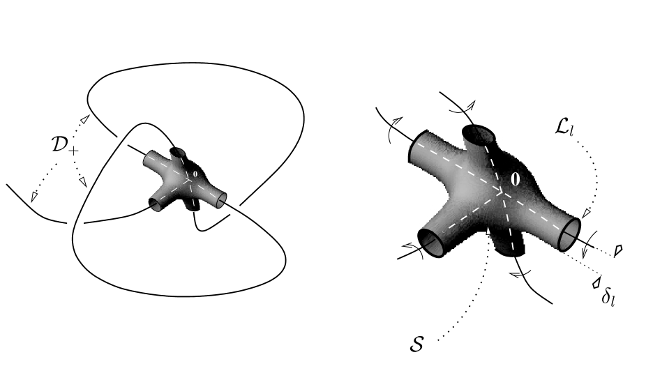
Figure 2: Example of a set $\mathcal{D}_{+}$ in the presence of constraints. On the left part of the figure is displayed a closed Dirac string crossing itself once at $\mathbf{r}=\mathbf{0}$, in addition to a half Dirac string. From a global perspective, one can predict that the former will not contribute to the monopole charge. Nevertheless, in a neighborhood of $\mathbf{r}=\mathbf{0}$ (right figure) one has to compute the winding of $\mathcal{Z}_{l}$ when $\mathbf{r}$ traverses $\mathcal{L}_{l}$ for each of the five half-strings.

Since $\mathcal{L}$ can be taken arbitrarily close to $\mathcal{D}_{+}$, and not intersecting $\mathcal{D}_{-}$, we have

$$\frac{e_{z}(\mathbf{r})}{e(\mathbf{r})}=1+O(\delta_{l})\quad\mathrm{when}\quad\mathbf{r}\in\mathcal{L}_{l}\;.$$ (13)

From this it follows that

$$g=\lim_{\mathcal{S}\to\text{closed sphere}}\frac{\Delta\Phi}{4\pi}\ =\frac{1}{2}\sum_{l=1}^{N}w_{l}\;,$$ (14)

where

$$w_{l}\stackrel{{\scriptstyle\mbox{\rm\scriptsize def}}}{{=}}\frac{1}{2\pi}\ \oint_{\mathcal{L}_{l}}\;\frac{e_{y}\boldsymbol{\nabla_{\!r}}\,e_{x}-e_{x}\boldsymbol{\nabla_{\!r}}\,e_{y}}{e_{x}^{2}+e_{y}^{2}}\;d\mathbf{l}_{l}\;.$$ (15)

$w_{l}$ has a natural topological interpretation. It is the algebraic winding number of the complex number

$$\mathsf{Z}_{l}(\mathbf{r})\stackrel{{\scriptstyle\mbox{\rm\scriptsize def}}}{{=}}e_{x}(\mathbf{r})+\mathrm{i}\,e_{y}(\mathbf{r})$$ (16)

when $\mathbf{r}$ traverses $\mathcal{L}_{l}$. It is a well defined quantity: $\mathsf{Z}_{l}(\mathbf{r})$ never crosses zero because $\mathbf{r}$ never touches $\mathcal{D}$.

Eq. (14) yields an alternative interpretation of the charge as a sum of winding numbers associated to the Dirac strings. It also provides a method to compute the charge, or to generate arbitrary values.

5 Two examples

We end up by illustrating the procedure with several examples (the generic case of section 3 is similar to the second one). In all the cases described below, we will Taylor expand e near the origin and suppose that the terms that we explicitly retain are sufficient to fix the local geometry of $\mathcal{D}$ completely.

5.1 An example with two choices of gauge

Consider a case where in a suitable choice of coordinates we have,

$$\text{e}(x,y,z)\ =\ [x^{2}+z,y^{2}+z,z]+\text{higher order terms}\;.$$ (17)

It follows immediately that $\mathcal{D}_{+}=\{\mathbf{0}\}$ so that $g=0$. To illustrate the importance of the gauge, we now treat the same example but in a gauge that exchanges $\mathcal{D}_{+}$ and $\mathcal{D}_{-}$. $\mathcal{D}_{-}$ is made of four half branches of parabolae: $\bigl{\{}[x=\pm\sqrt{-z},y=\pm\sqrt{-z},z\leq 0]\bigr{\}}$. Close enough to $\mathbf{r}=\mathbf{0}$ they can be assimilated to their tangent, i.e. the two axes $\{x=\pm y,z=0\}$. The surface $\mathcal{S}$ looks topologically like the one in figure 3.

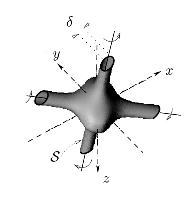
Figure 3: Near $\mathbf{r}=\mathbf{0}$, the Dirac strings in $\mathcal{D}_{-}$ are tangent to the two straight lines $x=\pm y$, and the four loops $\mathcal{L}_{l}$ are circles of radius $\delta$ and constant $y$ with center in one of the lines.

The four small loops $\mathcal{L}_{l}$ can be chosen to be centered on $\mathcal{D}_{-}$ and parametrized by $[x=\pm\epsilon+\delta\cos\theta,y=\pm\epsilon,z=-\epsilon^{2}-\mathrm{sgn}(y)\delta\sin\theta]$. $\theta$ runs from $0$ to $2\pi$, whereas $\epsilon$ and $\delta$ are fixed and small strictly positive quantities measuring the distance to the origin and the radius of the loops, respectively. From the definitions (16) and (17) we get $\mathsf{Z}=\delta[-\mathrm{sgn}(y)(1+\mathrm{i})\sin\theta+2\ \mathrm{sgn}(x)\epsilon\cos\theta]+O(\delta^{2})$. $\mathsf{Z}$ describes (a small perturbation of) an ellipse centered at the origin whose great axis is the segment $[-\delta(1+\mathrm{i}),\delta(1+\mathrm{i})]$ and whose width is proportional to $\epsilon$. The corresponding winding number is $\mathrm{sgn}(x)\mathrm{sgn}(y)$ and therefore the total charge given by (14) vanishes.

5.2 An example with a finite but arbitrarily large number of constraints

Now consider the case

$$\text{e}(x,y,z)\ =\ [(xy)^{n},\frac{1}{2}(x^{2n}-y^{2n}),z]+\text{higher order terms}\ ,$$ (18)

where $n$ is a strictly positive integer. The propagation of light in a twisted anisotropic dielectric medium considered in [Berry86a, see eq. (45)] corresponds to $n=1$. $\mathcal{D}_{+}$ is the half-axis $x=y=0,z\geq 0$. There is only one loop to consider (see figure 4).

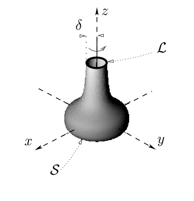
Figure 4: The examples considered in section 5.2 and 6 lead to one half Dirac string $x=y=0$ and $z\geq 0$.

Let us fix $z=z_{0}\geq 0$ and $\delta>0$. Consider the loop

$$\mathcal{L}\equiv[x=\delta\cos\theta,y=\delta\sin\theta,z=z_{0}],\qquad\theta\in[0,2\pi[\;.$$ (19)

Then $\Delta\Phi/(2\pi)$ is the winding number around zero of

$$\mathsf{Z}(\theta)=\delta^{2n}\left[\left(\frac{\sin(2\theta)}{2}\right)^{n}+\frac{\mathrm{i}}{2}\,\bigl{(}\cos^{2n}\theta-\sin^{2n}\theta\bigr{)}\right]\ .$$ (20)

If $n$ is even there is no winding, since the real part of $\mathsf{Z}$ remains always positive. Therefore $g=0$. In contrast, if $n$ is odd $\mathsf{Z}(\theta)$ winds clockwise twice, and therefore $g=-2g_{0}$. Figure 5 illustrates two different contact points corresponding to the two possible charges.

6 Arbitrarily large charges

In order to get arbitrarily large winding numbers for $\mathsf{Z}$, we make use of Chebyshev’s polynomials, defined by [Magnus+66a, chap.V, §5.7]

$$\mathsf{C}_{n}(q)=\cos(n\arccos q)=\frac{1}{2}\left[\left(q+\mathrm{i}\sqrt{1-q^{2}}\right)^{n}+\left(q-\mathrm{i}\sqrt{1-q^{2}}\right)^{n}\right]\;,$$ (21)

where $n$ is an arbitrary integer and $q$ a real number satisfying $-1\leq q\leq 1$. Let us take

$$\text{e}(x,y,z)\ =\ \begin{pmatrix}\displaystyle f(\sqrt{x^{2}+y^{2}})\ \mathsf{C}_{n}\!\!\left[\frac{x}{\sqrt{x^{2}+y^{2}}}\right]\\[21.52771pt] \displaystyle g(\sqrt{x^{2}+y^{2}})\ \mathsf{C}_{n}\!\!\left[\cos\left(\frac{\pi}{2n}\right)\frac{x}{\sqrt{x^{2}+y^{2}}}+\sin\left(\frac{\pi}{2n}\right)\frac{y}{\sqrt{x^{2}+y^{2}}}\right]\\[21.52771pt] \displaystyle z\end{pmatrix}+\text{higher order terms}\;.$$ (22)

$f(q)$ and $g(q)$ are some regularizing real functions that vanish at $q=0$ faster than any singular denominator coming from $\mathsf{C}_{n}$. An appropriate choice is, for instance, $f(q)=g(q)=q^{n}$. Though $\mathsf{C}_{n}$ vanishes $n$ times in $[-1,1]$, one can always choose a small neighborhood where $\mathbf{r}=\mathbf{0}$ is the unique point in $\mathcal{M}$. As in the last example, the set $\mathcal{D}_{+}$ is made of one Dirac half string on the half-axis $x=y=0,z\geq 0$. Constructing the same loop as before one gets

$$\mathsf{Z}(\theta)=f(\delta)\cos(n\theta)+\mathrm{i}\,g(\delta)\sin(n\theta)\ ,$$ (23)

which corresponds to $g=ng_{0}$. This provides an explicit example of a monopole carrying an arbitrarily large charge, and therefore creating arbitrarily large phase shifts for a loop located close to the degeneracy in parameter space. The contact between energy surfaces with $n=2$ is illustrated in part (a) of figure 5, which is identical to the geometry of the contact defined by Eq.(18) with $n=1$ (up to an irrelevant scaling factor).

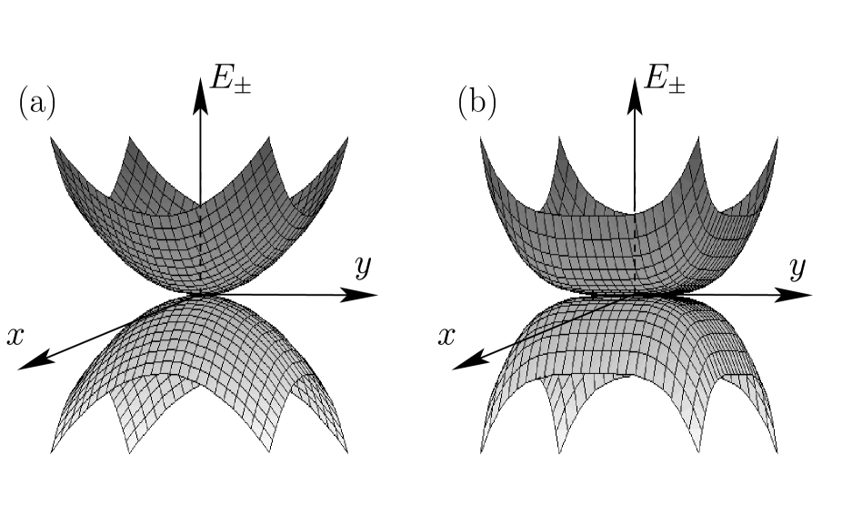
Figure 5: Geometry of the contact point between energy surfaces for $z=0$. Part (a) corresponds to Eq.(18) with $n=1$ and to Eq.(22) with $n=2$. The charge is $g/g_{0}=2$. Part (b) corresponds to Eq.(18) with $n=2$. The charge vanishes. Notice the difference in the geometry of the contact between both cases.

7 Discussion

Spectral degeneracies with charges higher than one have been observed in several contexts. For instance, via the variations of Chern numbers in quantum systems with mixed and chaotic classical dynamics [Leboeuf+90a, Leboeuf+92a]. These integer topological invariants measure the transport (Hall conductivity) of each band of a doubly periodic system. Values of $g/g_{0}=2$ and $3$ were found (cf in Fig. 2 of Ref. [Leboeuf+90a] the contact points at $\gamma=0.7106$ between the second and third levels, and at $\gamma=0.4477$ between the fourth and fifth levels, respectively). A closer analysis of the geometry of the contact points reveals that these two degeneracies coincide with the parabolic and cubic contacts described by Eq.(22) with $n=2$ and $3$, respectively. For instance, the $g/g_{0}=2$ contact is parabolic in the Bloch angles and linear in the parameter $\gamma$.

We have also exhibited the possibility of having a contact point with total charge equal to zero. Although its presence will in general be difficult to detect, it would be interesting to find an explicit quantum mechanical model displaying this curious feature.

In the electromagnetic analogy based on the general formula, the “sources” of the geometric phase in parameter space are the spectral degeneracies plus some additional currents not related to them. In the particular (and generic) case of a diabolical contact, the contribution of the degeneracy is simple: it acts as a pure monopole charge, thus contributing to $\mathrm{div}\,\mathbf{B}$ but not to $\mathbf{curl}\,\mathbf{B}$. However, for an arbitrary contact point – defined by Eq.(8) – the situation is different. On the one hand, the divergence of $\mathbf{B}$ is not simply determined by a charge, but more generally by a charge distribution (cf Eq.(11)). The latter can contain higher multipole moments. Moreover, the $\mathrm{curl}$ of $\mathbf{B}$ need not be zero. In the present study, we have only considered a particular aspect of the sources of geometric phase associated to the field produced by a degeneracy, namely the total charge of the distribution. A more complete classification scheme is clearly needed.

References

- [1] \harvarditemBerry1984Berry84a Berry M V 1984 Proc. Roy. Soc. London Ser. A 392, 45–57. Reprinted in [Shapere/Wilczek89a].
- [2] \harvarditemBerry1986Berry86a Berry M V 1986 in V Gorini & A Frigerio, eds, ‘Fundamental aspects of quantum theory’ Vol. B144 of NATO ASI Series (physics) Proc. of ARW, Villa Olmo/Como (Italy), 1985 Plenum New York pp. 267–278.
- [3] \harvarditemDirac1931Dirac31a Dirac P A M 1931 Proc. Roy. Soc. London Ser. A 133, 60–72.
- [4] \harvarditemDirac1978Dirac78a Dirac P A M 1978 Directions in Physics lectures delivered during a visit to Australia and New Zealand—August/September 1975 John Wiley and sons, Inc. New York.
- [5] \harvarditemFaure & Leboeuf1993Faure/Leboeuf93a Faure F & Leboeuf P 1993 in G. F Dell’Antonio, S Fantoni & V. R Manfredi, eds, ‘Proceedings of the Workshop: From Classical to Quantum Chaos, Trieste, Italy’ Vol. 41 Conference Prooceedings SIF Bologna pp. 75–97.
- [6] \harvarditemKnox & Gold1964Knox/Gold64a Knox R S & Gold A 1964 Symmetry in the solid state Lecture notes and supplements in physics W. A. Benjamin, Inc New York.
- [7] \harvarditemLeboeuf et al.1990Leboeuf+90a Leboeuf P, Kurchan J, Feingold M & Arovas D P 1990 Phys. Rev. Lett. 65(25), 3076–3079.
- [8] \harvarditemLeboeuf et al.1992Leboeuf+92a Leboeuf P, Kurchan J, Feingold M & Arovas D P 1992 Chaos 2(1), 125–130.
- [9] \harvarditemMagnus et al.1966Magnus+66a Magnus W, Oberhettinger F & Soni R P 1966 Formulas and Theorems for the Special Functions of Mathematical Physics Springer-Verlag Berlin. (3rd edition).
- [10] \harvarditemShapere & Wilczek1989Shapere/Wilczek89a Shapere A & Wilczek F, eds 1989 Geometric Phases in Physics Vol. 5 of Advanced Series in Mathematical Physics World Scientific Singapore.
- [11] \harvarditemSimon1983Simon83a Simon B 1983 Phys. Rev. Lett. 51(24), 2167–2170. Reprinted in [Shapere/Wilczek89a].
- [12] \harvarditemStone1976Stone76a Stone A J 1976 Proc. Roy. Soc. London Ser. A 351, 141–150. Reprinted in [Shapere/Wilczek89a].
- [13] \harvarditemvon Neumann & Wigner1929vonNeumann/Wigner29a von Neumann J & Wigner E 1929 Phys. Z. 30, 467–470. English translation in [Knox/Gold64a] pp. 167–172: On the Behavior of the Eigenvalues in Adiabatic Processes.
- [14]