Finite-Time Disentanglement via Spontaneous Emission

Abstract

We show that under the influence of pure vacuum noise two entangled qubits become completely disentangled in a finite time, and in a specific example we find the time to be given by $\ln\Big{(}\frac{2+\sqrt{2}}{2}\Big{)}$ times the usual spontaneous lifetime.

Superposition and entanglement are two basic features that distinguish the quantum world from the classical world. While quantum coherence is recognized as a major resource, decoherence due to the interaction with an environment is a crucial issue that is of fundamental interest defdeco ; zeh ; str ; ah . When coherence exists among several distinct quantum subsystems the issue becomes more complicated because, along with the local coherence of each constituent particle, their entanglement brings a special kind of distributed or nonlocal coherence. It is this distributed coherence that really matters in many important applications of quantum information preskill ; mc . Consequently, the fragility of nonlocal quantum coherence is recognized as a main obstacle to realizing quantum computing and quantum information processing (QIP) viola1 ; plk . Apart from the important link to QIP realizations, a deeper understanding of entanglement decoherence is also expected to lead to new insights into quantum fundamentals, particularly quantum measurement and the quantum-classical transition gisin1 ; hal ; dio . Although quantum decoherence has been extensively studied in recent years, it remains unclear how a local decoherence rate is related to a nonlocal disentanglement rate when a multi-particle quantum state is in contact with one or more noisy environments.

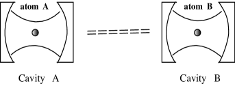
Figure 1: Schematic illustration of a set-up in which two atoms are located inside two spatially separated cavities A and B. The two atoms are initially entangled but have no direct interaction afterwards.

Therefore, a deep understanding of the decoherence in any viable realization of qubits is desirable and it is surprising that few if any fundamental treatments exist of decoherence that include the dynamics of disentanglement on better than an empirical or phenomenological basis.

Here we consider two initially entangled qubits and examine the dynamics of their disentanglement due to spontaneous emission without phenomenological approximation. There is perhaps no simpler realistic bipartite model in which all of the effects of quantum noise can be considered fully analytically. We show that decoherence caused by vacuum fluctuations can affect localized and distributed coherences in very different ways. As one surprising consequence, we show that spontaneous disentanglement may take only a finite time to be completed, while local decoherence (the normal single-atom transverse and longitudinal decay) takes an infinite time.

To make our model and results concrete, we restrict our attention to two two-level atoms $A$ and $B$ coupled individually to two cavities which are initially in their vacuum states (see Fig.  1). In the general framework of system-plus-environment, the two two-level atoms are identified as the system of interest, whereas the two cavities serve as the environments. The interaction between each atom and its environment results in the loss of both local coherence and quantum entanglement of the two atoms. In its simplest form such a model may be formulated with the following total Hamiltonian, which is given by (we set $\hbar=1$): $H_{\rm tot}=H_{\rm at}+H_{\rm int}+H_{\rm cav}$, where the Hamiltonian of the two atoms $H_{\rm at}$, the two cavities $H_{\rm cav}$ and the interaction $H_{\rm int}$ are given by

$$H_{\rm at} = \frac{1}{2}\omega_{A}\sigma^{A}_{z}+\frac{1}{2}\omega_{B}\sigma^{B}_{z}$$ (1)

$$H_{\rm cav} = \sum_{\bm{k}}\omega_{\bm{k}}a_{\bm{k}}^{\dagger}a_{\bm{k}}+\sum_{\bm{k}}\nu_{\bm{k}}b_{\bm{k}}^{\dagger}b_{\bm{k}}$$ (2)

$$H_{\rm int} = \sum_{{\bm{k}}}(g^{*}_{\bm{k}}\sigma^{A}_{-}a^{\dagger}_{\bm{k}}+g_{\bm{k}}\sigma^{A}_{+}a_{\bm{k}})$$ (3)

$$+ \sum_{{\bm{k}}}(f^{*}_{\bm{k}}\sigma^{B}_{-}b^{\dagger}_{\bm{k}}+f_{\bm{k}}\sigma^{B}_{+}b_{\bm{k}})$$

where $g_{\bm{k}},f_{\bm{k}}$ are coupling constants and $\sigma_{z}$ denotes the usual diagonal Pauli matrix, and the standard 2-qubit product basis is given by:

$$|1\rangle_{AB} = |++\rangle_{AB},\quad|2\rangle_{AB}=|+-\rangle_{AB},$$

$$|3\rangle_{AB} = |-+\rangle_{AB},\quad|4\rangle_{AB}=|--\rangle_{AB},$$ (4)

where $|\pm\pm\rangle_{AB}\equiv|\pm\rangle_{A}\otimes|\pm\rangle_{B}$ denote the eigenstates of the product Pauli spin operator $\sigma_{z}^{A}\otimes\sigma_{z}^{B}$ with eigenvalues $\pm 1$. The total Hamiltonian, given by equations (1)-(3), provides us an important solvable model of the atom-field interaction in quantum optics.

Suppose that initially the atoms are entangled with each other but not with the cavities, i.e., we assume that at $t=0$ the two atoms and the cavities are described by the product state,

$$|\Psi_{\rm tot}\rangle=|\psi\rangle_{AB}\otimes|0\rangle_{A}|0\rangle_{B},$$ (5)

where $|\psi\rangle_{AB}$ is the entangled initial state of the two atoms and $|0\rangle_{A}|0\rangle_{B}$ is the vacuum state of two cavities. For simplicity, we will not take into account the spatial degrees of freedom of the two atoms. The convolutionless master equation of the system of two atoms can be obtained as follows com0 :

$$\frac{d}{dt}\rho = -i[H^{\prime}_{\rm at}(t),\rho]$$ (6)

$$+F_{R}(t)\Big{(}[\sigma_{-}^{A},\rho_{t}\sigma_{+}^{A}]+[\sigma_{-}^{A}\rho_{t},\sigma_{+}^{A}]\Big{)}$$

$$+G_{R}(t)\Big{(}[\sigma_{-}^{B},\rho_{t}\sigma_{+}^{B}]+[\sigma_{-}^{B}\rho_{t},\sigma_{+}^{B}]\Big{)}$$

where $H^{\prime}_{\rm at}(t)$ is the system Hamiltonian modified to take into account the Lamb shifts

$$H^{\prime}_{\rm at}(t)=\frac{1}{2}(\omega_{A}+F_{I}(t))\sigma^{A}_{z}+\frac{1}{2}(\omega_{B}+G_{I}(t))\sigma^{B}_{z}$$ (7)

and the coefficients $F_{R,I}$ and $G_{R,I}$ are the real and imaginary parts of $F(t)$ and $G(t)$, which are given by

$$F(t) = \frac{1}{b(t)}\int^{t}_{0}ds\alpha(t-s)b(s)$$ (8)

$$G(t) = \frac{1}{c(t)}\int^{t}_{0}ds\beta(t-s)c(s)$$ (9)

Note that the cavity correlation functions are

$$\alpha(t-s) = \sum_{\bm{k}}|g_{\bm{k}}|^{2}e^{-i\omega_{\bm{k}}(t-s)}$$ (10)

$$\beta(t-s) = \sum_{\bm{k}}|f_{\bm{k}}|^{2}e^{-i\nu_{\bm{k}}(t-s)}$$ (11)

and the functions $b(s)$ and $c(s)$ are the fundamental solutions of the equations of motion:

$$\dot{b}(s) + i\omega_{A}b(s)+\int^{s}_{0}d\lambda\alpha(s-\lambda)b(\lambda)=0$$ (12)

$$\dot{c}(s) + i\omega_{B}c(s)+\int^{s}_{0}d\lambda\beta(s-\lambda)c(\lambda)=0$$ (13)

The master equation (6) is extremely useful for the study of decoherence, and for the purpose of disentanglement analysis it will be very convenient to find an explicit expression for its solution. In the interaction picture, where

$$\tilde{\rho}(t)=e^{i\int^{t}_{0}H^{\prime}_{\rm at}(s)ds}\rho(t)e^{-i\int^{t}_{0}H^{\prime}_{\rm at}(s)ds},$$ (14)

the general solutions of equation (6) can be described in terms of a Kraus representation preskill ; mc ; kra ; wk . As can be seen below, the Kraus representation allows a very elegant analysis of the disentanglement time for arbitrary states. Precisely, for any initial state $\rho(0)$, the density operator at $t$ can be expressed ascom

$$\tilde{\rho}(t)=\sum_{\mu=1}^{4}K_{\mu}(t)\rho(0)K^{\dagger}_{\mu}(t),$$ (15)

where the Kraus operators $K_{\mu}(t)$ satisfy $\sum_{\mu}K^{\dagger}_{\mu}K_{\mu}=I$ for all $t$. The Kraus operators for this model are given by

$$K_{1} = \left(\begin{array}[]{clcr}\gamma_{A}&&0\\ 0&&1\\ \end{array}\right)\otimes\left(\begin{array}[]{clcr}\gamma_{B}&0\\ 0&1\\ \end{array}\right),$$ (20)

$$K_{2} = \left(\begin{array}[]{clcr}\gamma_{A}&&0\\ 0&&1\\ \end{array}\right)\otimes\left(\begin{array}[]{clcr}0&0\\ \omega_{B}&0\\ \end{array}\right),$$ (25)

$$K_{3} = \left(\begin{array}[]{clcr}0&0\\ \omega_{A}&0\\ \end{array}\right)\otimes\left(\begin{array}[]{clcr}\gamma_{B}&0\\ 0&1\\ \end{array}\right),$$ (30)

$$K_{4} = \left(\begin{array}[]{clcr}0&0\\ \omega_{A}&0\\ \end{array}\right)\otimes\left(\begin{array}[]{clcr}0&0\\ \omega_{B}&0\\ \end{array}\right),$$ (35)

and the time-dependent Kraus matrix elements are

$$\gamma_{A}(t) = \exp\left[{-\int^{t}_{0}dsF_{R}(s)}\right],$$ (36)

$$\gamma_{B}(t) = \exp\left[{-\int^{t}_{0}dsG_{R}(s)}\right],$$ (37)

$$\omega_{A}(t) = \sqrt{1-\gamma^{2}_{A}(t)},\,\,\,\,\omega_{B}(t)=\sqrt{1-\gamma^{2}_{B}(t)}$$ (38)

With the preceding discussion, we are now in a position to determine both the local decoherence rate and the disentanglement rate. Multiple interpretations of the term decoherence in the literature can lead to confusion, so we will use global or non-local decoherence (or disentanglement) here when we refer to loss of bipartite entanglement. The terms local decoherence or local relaxation will refer to longitudinal and transverse decay of single-atom density matrix elements. In the present example local and non-local decoherence both arise from the effects of spontaneous emission and in that sense are not independent.

We begin with the coherence decay of a single qubit under the master equation (6). The local decoherence rates of the qubits can be estimated from the reduced density matrices $\rho^{A}\equiv{\rm Tr}_{B}\{\rho\}\quad{\rm and}\quad\rho^{B}\equiv{\rm Tr}_{A}\{\rho\}$. The local decoherence rates are determined by the well-known Bloch equations with general time-dependent functions $F(s),G(s)$. For example,

$$\langle\dot{\sigma}^{A}_{-}\rangle=-\left[F(t)+i\omega_{A}\right]\langle\sigma^{A}_{-}\rangle$$ (39)

and $\langle\dot{\sigma}^{A}_{+}\rangle=\langle\dot{\sigma}^{A}_{-}\rangle^{*}$, where $\sigma^{A}_{-}=\sigma_{-}\otimes I$. Similar equations hold for $\sigma_{\pm}^{B}$. Hence we have

$$|\langle\sigma^{A}_{\pm}(t)\rangle| = |\langle\sigma^{A}_{\pm}(0)\rangle|e^{-\int^{t}_{0}dsF_{R}(s)},$$ (40)

$$|\langle\sigma^{B}_{\pm}(t)\rangle| = |\langle\sigma^{B}_{\pm}(0)\rangle|e^{-\int^{t}_{0}dsG_{R}(s)}.$$ (41)

Given these equations, local decoherence behaviors are determined by the character of the functions $F_{R}(t)$ and $G_{R}(t)$ which we always assume to be positive functions asymptotically. In the familiar Born-Markov approximation one has purely exponential decay with rates given by $F(t)\rightarrow\Gamma_{A}/2$ and $G(t)\rightarrow\Gamma_{B}/2$, where the $\Gamma$’s are the Einstein A coefficients for the two-level atoms in the cavities.

The comparison of interest is with the disentanglement rate. Since entanglement decoherence processes are most generally associated with mixed states, we will use Wootters’s concurrence to quantify the degree of entanglement woo . The concurrence is conveniently defined for both pure and mixed states. Let $\rho$ be a density matrix of the pair of atoms expressed in the standard basis (Finite-Time Disentanglement via Spontaneous Emission). The concurrence may be calculated explicitly from the density matrix $\rho$ for qubits A and B: $C(\rho)=\max\left(0,\sqrt{\lambda_{1}}-\sqrt{\lambda_{2}}-\sqrt{\lambda_{3}}-\sqrt{\lambda_{4}}\,\,\right),$ where the quantities $\lambda_{i}$ are the eigenvalues of the matrix $\zeta$:

$$\zeta\equiv\rho(\sigma^{A}_{y}\otimes\sigma^{B}_{y})\rho^{*}(\sigma^{A}_{y}\otimes\sigma^{B}_{y}),$$ (42)

arranged in decreasing order. Here $\rho^{*}$ denotes the complex conjugation of $\rho$ in the standard basis (Finite-Time Disentanglement via Spontaneous Emission) and $\sigma_{y}$ is the usual (pure imaginary) Pauli matrix expressed in the same basis. It can be shown that the concurrence varies from $C=0$ for a disentangled state to $C=1$ for a maximally entangled state.

We now show two categories of result for entanglement decay. In the first more general category we show that, for all entangled (possibly mixed) states, entanglement decays not only more rapidly than the fastest decoherence rate of an individual qubit, but at least as fast as the sum of the separate rates. In the second category we present a sharper result in a specific mixed state example, in which the entanglement goes exactly to zero in a finite time and remains zero. Both categories of result are a consequence of normal spontaneous emission.

For the first category of result, let us note that the concurrence $C(\rho)$ is a convex function of $\rho$ woo . From (15), one immediately has

$$C(\rho(t))\leq\sum_{\mu=1}^{4}C(K_{\mu}\rho(0)K^{\dagger}_{\mu}),$$ (43)

where $K_{\mu}$ are defined in equations (20) to (35). Let us consider a typical term $C(K_{\mu}\rho(0)K^{\dagger}_{\mu})$ in (43) and denote it by $\rho_{\mu}=K_{\mu}\rho(0)K^{\dagger}_{\mu}.$ From the definition of concurrence, it can be proved that

$$C(\rho_{1}) = e^{-\int^{t}_{0}(F_{R}(s)+G_{R}(s))ds}C(\rho(0)),$$ (44)

$$C(\rho_{\mu}) = 0,\,\,\mu=2,3,4.$$ (45)

Then the inequality (43) immediately leads to,

$$C(\rho(t)) \leq e^{-\int^{t}_{0}(F_{R}(s)+G_{R}(s))ds}C(\rho(0)),$$ (46)

which establishes the first result mentioned. It is not difficult to show that the upper bound is the minimal upper bound. To treat the disentanglement process in general and more completely requires a discussion of the asymptotic behavior of the functions $F_{R}(s)$ and $G_{R}(s)$, which is beyond the scope of the present paper.

In what follows we develop the second result mentioned above. We show that within the general result there are very unusual and striking specific consequences. One example shows that, within the general exponential character evident in (46), disentanglement can be completed in a finite time while the local decoherences need an infinite time. Let us assume that the initial density matrix is only partially coherent, but include an arbitrary degree of non-local coherence of a familiar type (one of the atoms is excited, but it is not certain which one). This is easily expressed in the following form cav

$$\rho=\frac{1}{3}\begin{pmatrix}a(t)&0&0&0\\ 0&b(t)&z(t)&0\\ 0&z^{*}(t)&c(t)&0\\ 0&0&0&d(t)\end{pmatrix},$$ (47)

where the factor 1/3 is for notational convenience. The concurrence for this density matrix is $C=\frac{2}{3}\max\{0,\,\,|z|-\sqrt{ad}\}$. For simplicity, we consider an important class of mixed states with a single parameter $a$ satisfying initially $a\geq 0,\ d=1-a$, and $b=c=z=1$, so then initially $C(\rho(0))=\frac{2}{3}[1-\sqrt{a(1-a)}]$. For $t\geq 0$ the matrix elements are given by

$$a(t) = \gamma^{2}_{A}\gamma^{2}_{B}a,$$ (48)

$$b(t) = \gamma_{A}^{2}+\gamma_{A}^{2}\omega^{2}_{B}a,$$ (49)

$$c(t) = \gamma_{B}^{2}+\omega^{2}_{A}\gamma^{2}_{B}a,$$ (50)

$$d(t) = 1-a+\omega_{A}^{2}+\omega_{B}^{2}+\omega^{2}_{A}\omega_{B}^{2}a,$$ (51)

$$z(t) = \gamma_{A}\gamma_{B}.$$ (52)

To simplify the calculations, we use the Markov limit results and assume the cavities are similar so $\gamma_{A}=\gamma_{B}=\gamma=\exp[-\Gamma t/2],$ and $\omega_{A}=\omega_{B}=\omega=\sqrt{1-\exp[-\Gamma t]}.$ The concurrence for the density matrix $\rho(t)$ is given by

$$C(\rho(t))=\frac{2}{3}\max\{0,\gamma^{2}f(t)\}$$ (53)

where $f(t)=1-\sqrt{a\left(1-a+2\omega^{2}+\omega^{4}a\right)}.$ The sufficient condition for the concurrence (53) to be zero is

$$1-a(1-a+2\omega^{2}+\omega^{4}a)\leq 0.$$ (54)

The simplest case is $a=1$ and from this we can easily show the surprising result that the density matrix (47) has a finite disentanglement time. That is, $C(\rho(t))\equiv 0$ for all $t\geq t_{d}$, where $t_{d}$ is very finite:

$$t_{d}\equiv\frac{1}{\Gamma}\ln\left[\frac{2+\sqrt{2}}{2}\right].$$ (55)

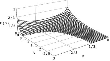
Figure 2: This figure shows the entanglement decay via spontaneous emission starting from the initially entangled states (47) with $a$ between zero and 1, $d=1-a$ and $b=c=z=1$. Finite-time complete disentanglement takes place for $a>1/3$, and when $a\leq 1/3$ disentanglement of the initial state is only completed asymptotically.

In response to this surprising result, a natural question will be: does spontaneous emission cause all initially entangled two-qubit states to disentangle at some finite critical time? The answer is no. To see this, we consider the entire range of different $a$ values, and plot the concurrence decay in Fig. 2. The figure shows that for all $a$ values between 1/3 and 1 concurrence decay is completed in a finite time, but for smaller $a$’s the time for complete decay is infinite. The different behaviors exhibited over the allowed range of $a$ values in Fig. 2 show that our two-level atom model behaves qualitatively differently from the continuous variable two-atom model discussed in hal by Dodd and Halliwell. In that case all initially entangled states become separable after a finite time (see also rus ).

To summarize, we have shown for the physically fundamental and unavoidable process of spontaneous emission that nonlocal disentanglement times are shorter than local decoherence times for arbitrary entangled states (pure or mixed). We based our results on perhaps the simplest realistic decoherence scenario in which two entangled qubits individually interact with vacuum noise. The model allows an exact analysis and also shows, remarkably, that complete disentanglement can be reached after only a finite time, whereas more familiar local decoherence processes take an infinite time to be complete. We believe our results are of generic nature. Undoubtedly a deep understanding of the relation between decoherence and disentanglement will be of importance for both the foundation of quantum mechanics and practical quantum information applications.

We acknowledge constructive correspondence with J. Halliwell and K. Wodkiewicz, and assistance with Fig. 2 from C. Broadbent. We have obtained financial support from NSF Grants PHY-9415582 and PHY-0072359 and important assistance from L.J. Wang of the NEC Research Institute.

References

- (1) W. H. Zurek, Phys. Today 44 (10), 36 (1991); Phys. Rev. D 24, 1516 (1981); 26, 1862 (1982); Prog. Theor. Phys. 89, 281 (1993).
- (2) E. Joos and H. D. Zeh, Z. Phys. B 59, 223 (1985).
- (3) D. Braun, F. Haake, and W. T. Strunz, Phys. Rev. Lett. 86, 2913 (2001).
- (4) C. Anastopoulos and B. L. Hu, Phys. Rev. A 62, 033821 (2000).
-
(5)
J. Preskill, Lecture Notes on Quantum
Information and Quantum Computation
at www.theory.caltech.edupeoplepreskillph229. - (6) M. A. Nielson and I. L. Chuang, Quantum Computation and Quantum Information (Cambridge, England, 2000).
- (7) L. Viola, E. Knill, and S. Lloyd, Phys. Rev. Lett. 83, 4888 (1999).
- (8) A. Beige, D. Braun, B. Tregenna, and P. L. Knight, Phys. Rev. Lett. 85, 1762 (2001).
- (9) N. Gisin, Phys Lett A 210, 151 (1996) and references therein.
- (10) P. J. Dodd and J. J. Halliwell, Phys. Rev. A 69 , 052105 (2004); P. J. Dodd, Phys. Rev. A 69, 052106 (2004).
- (11) L. Diosi, in Irreversible Quantum Dynamics, edited by F. Benatti and R. Floreanini (Springer, Berlin, 2003).
- (12) The derivation and memory effects depicted by and of the master equation will be discussed elsewhere. In this paper, the use of the master equation is limited to the Markov approximation, that is, the correlation functions are functions: and .
- (13) K. Kraus, States, Effect, and Operations: Fundamental Notions in Quantum Theory (Springer-Verlag, Berlin, 1983).
- (14) K. Wódkiewicz, Opt. Express 8, No. 2, 145 (2001); S. Daffer, K. Wódkiewicz, and J. McIver, quant-ph/0211001, (2002). S. Daffer, K. Wódkiewicz, J. D. Cresser, and J. K. McIver, quant-ph/0309081, (2003).
- (15) In this paper, we always assume and to be positive functions. If take negative values, in equation (15) must be replaced with the transpose matrix .
- (16) S. Hill and W. K. Wootters, Phys. Rev. Lett. 78, 5022 (1997); W. K. Wootters, Phys. Rev. Lett. 80, 2245 (1998).
- (17) Preparation of mixed entangled states between the two atoms located in a spatially separated cavities by using QED cavity techniques has been discussed, e.g., see: S. Bose, P. L. Knight, M. B. Plenio and V. Vedral, Phys. Rev. Lett. 83, 5158 (1999).
- (18) M. B. Ruskai, Preprint, arXiv: quant-ph/0302032, (2003).