A new mathematical representation of Game Theory I

Abstract

In this paper, we introduce a framework of new mathematical representation of Game Theory, including static classical game and static quantum game. The idea is to find a set of base vectors in every single-player strategy space and to define their inner product so as to form them as a Hilbert space, and then form a Hilbert space of system state. Basic ideas, concepts and formulas in Game Theory have been reexpressed in such a space of system state. This space provides more possible strategies than traditional classical game and traditional quantum game. So besides those two games, more games have been defined in different strategy spaces. All the games have been unified in the new representation and their relation has been discussed. General Nash Equilibrium for all the games has been proposed but without a general proof of the existence. Besides the theoretical description, ideas and technics from Statistical Physics, such as Kinetics Equation and Thermal Equilibrium can be easily incorporated into Game Theory through such a representation. This incorporation gives an endogenous method for refinement of Equilibrium State and some hits to simplify the calculation of Equilibrium State. The more privileges of this new representation depends on further application on more theoretical and real games. Here, almost all ideas and conclusions are shown by examples and argument, while, we wish, lately, we can give mathematical proof for most results.

Key Words: Game Theory, Quantum Game Theory, Quantum Mechanics, Statistical Physics

Pacs: 02.50.Le, 03.67.-a, 03.65.Yz, 05.20.-y, 05.30.-d

1 Introduction

Game Theory[1, 2] is a subject used to predict the strategy of all players in a game. The simplest game is static and non-cooperative game, which describe by payoff function $G$, a linear mapping from strategy space $S^{1}\times S^{2}\times\cdots S^{N}$ to N-dimension real space $\mathbb{R}^{N}$. For a game in mixture strategy space, in which every player uses mixture strategy $\vec{P}^{i}$, a probability distribution on strategy set $S^{i}$, Nash Theorem proves that there is always some mixture-strategy equilibrium points, on which no player has the willing to make an independent change. Therefor, such equilibrium points can be regarded as a converged points (or at least fixed points) of the system, then as the end state of all players.

On the other hand, Quantum Game Theory[3, 4] has been proposed as a quantum version of Game Theory[6, 5]. A typical two-player quantum game is defined as $\Gamma=\left(\mathcal{H},\rho_{0},S_{A},S_{B},P_{A},P_{B}\right)$, in which $\mathcal{H}$ is the Hilbert space of state of one quantum object, like a photon or electron. Such a quantum object plays an important role in Quantum Game Theory. The quantum strategy set $S_{A}$ or $S_{B}$ usually is defined as a set of unitary operator on state space $\mathcal{H}$, or sometimes subspace of $\mathcal{H}$. It’s believed that because quantum strategy space is usually larger than the corresponding classical strategy space, one can make use of such advantage of quantum strategy to make money over classical player. Generally speaking, a quantum game is not only a quantum version of a classical game. It describes the situation that every player plays game in a strategy space of quantum operators, which transform the state of a quantum object. Probably, someday, some original quantum games can be found alone this direction.

However, both of Classical Game Theory and Quantum Game Theory are expressed in single player strategy space, so the payoff function is a $\left(0,N\right)$ tensor $G^{i}\left(s^{1},s^{2},\dots,s^{N}\right)$, mapping a combination of $N$ single-player strategies onto a real number. On the contrary, in Quantum Statistical Mechanics, a matrix form of Hamiltonian $H$ is used in a any-particle case, and the form of density matrix of equilibrium state is always $\rho=e^{-\beta H}$. So a system-level description will unify our formulas for $N$-player game, and then maybe improve our understanding and calculation.

Starting from such an idea, in this paper, we construct a systematical way to reexpress everything into system-level description, including system state and its space, payoff matrix on system space, and reduced single-player payoff matrix. Then Canonical Quantum Ensemble distribution is used to describe system equilibrium state. So ideas and technics from Statistical Physics can be easily applied onto Game Theory. Such application implies a probability that a Kinetics Equation can be used to describe an evolution that a system ends at the equilibrium state starting from an arbitrary distribution. Because the traditional Game Theory only cares about the macro-equilibrium state, the Kinetics Equation approach is just pseudo-dynamical equation leading to the equilibrium state. The dynamical process itself might be meaningless.

Furthermore, besides providing a new pseudo-dynamical approach, the distribution function description has its own meaning. In Game Theory, maybe general for all economical subjects, usually it’s supposed that even the difference between two choices is very small, the high-value one is chosen. This is unnatural when the difference is smaller than the resolution of human decision. Therefor, we use a distribution function to replace the maximum-point solution. This means player $i$ will choose strategy $s^{i}_{\mu}$ with probability $e^{\beta E^{i}(s^{i}_{\mu})}$, even there are another strategy can make more money. Here, $\beta$ is the meaning of average resolution level, or in Statistical Physics, the average noise level. Unfortunately, although the ensemble description is the second topic of this paper, only some special case study has been investigated. A general form for any game is still waiting for more exploration.

Section $\S$2 constructs the new representation for classical and quantum game. Section $\S$3 use ensemble distribution and pseudo-dynamical approach to study the equilibrium state in this new representation. Discussion of relation between our new representation and quantum, and classical game is included in section $\S$2. A lot of questions are pointed out in the discussion section ($\S$4). Section $\S$5 is a short summary of the conclusions we have reached.

2 Mathematical Structure: Strategy Space, State Density Matrix and Payoff Matrix

Strategy set can be continuous and discrete, and this will effect the mathematical form of all variables, such as the state of player $i$ is $p(s^{i})$ or $p^{i}_{\mu}\delta(s^{i}-s^{i}_{\mu})$, and $G$ will be integrations or matrixes. In order to compare with the Mathematical form of Quantum Mechanics and point out the similarity, and to unify Classical Game Theory and Quantum Game Theory, here we use the discrete strategy, although the corresponding transformation of all ideas and formulas is quite straightforward. Most of our formulas and results can be generalized into $N$-player and $\left(\prod_{i=1}^{N}L_{i}\right)$-strategy game, so for simplicity of expressions, at most time, a $2$-player and $\left(L_{1}\times L_{2}\right)$-strategy game is used as our object.

2.1 The new representation of static classical game

For a $N$-player game, we suppose the strategy space of player $i$ is $S^{i}=\left\{s^{i}_{1},s^{i}_{2},\cdots,s^{i}_{L_{i}}\right\}$. The state of player $i$ is $\left|P^{i}\right>\equiv\left(p^{i}_{1},p^{i}_{2},\cdots,p^{i}_{L_{i}}\right)^{T}$ and $\sum_{\mu=1}^{L_{i}}p^{i}_{\mu}=1$. The payoff function of player $i$ is a $\left(0,N\right)$-tensor — a $N$-linear operator,

$$E^{i}(P^{1},P^{2},\dots,P^{N})=G^{i}\left(\left|P^{1}\right>,\left|P^{2}\right>,\cdots,\left|P^{N}\right>\right).$$ (1)

Specially, for a 2-player game, $G^{i}$ can be written as a matrix ($\left(0,2\right)$-tensor) so that

$$E^{i}(P^{1},P^{2})=\left<P^{1}\right|G^{i}\left|P^{2}\right>,$$ (2)

in which $G^{i}$ is $L_{1}\times L_{2}$ matrix, not necessary a square one. So a classical game is

$$\Gamma_{C}=\left(\left\{S^{i}\right\},\left\{G^{i}\right\}\right),$$ (3)

A general vector in $S^{i}$ can be defined as

$$\left|P^{i}\right>=\sum_{\mu=1}^{L_{i}}p^{i}_{\mu}\left|s^{i}_{\mu}\right>,$$ (4)

in which $\left\{s^{i}_{\mu}\right\}$ is the base vector set of strategy space $S^{i}$. Or in traditional language of Game Theory, it’s a set of all the pure strategies of player $i$.

Inspired by the application of Hilbert Space in Quantum Mechanics, now we introduce two ideas into Game Theory. First, to redefine the strategy space of single player as a Hilbert Space. Second, to use a system state to replace the single player state. Then, at the same time, a new form of payoff function is required to be equivalently defined on the system state.

A single-player state vector $\left|P^{i}\right>$ is written in a new form as

$$\rho^{i}=\sum_{\mu=1}^{L_{i}}p^{i}_{\mu}\left|s^{i}_{\mu}\right>\left<s^{i}_{\mu}\right|.$$ (5)

It’s density matrix form of a mixture state, because a classical strategy of player $i$ is to use strategy $s^{i}_{\mu}$ with probability $p^{i}_{\mu}$. The difference between equ(4) and equ(5) can be regarded as just to replace $\left|s^{i}_{\mu}\right>$ with $\left|s^{i}_{\mu}\right>\left<s^{i}_{\mu}\right|$. The reason of such replacement will be clear when we do it on quantum game. Actually, using density matrix to describe mixture state is a approach in Quantum Mechanics. A system state of all players is defined as

$$\rho^{s}=\prod_{i=1}^{N}\rho^{i}.$$ (6)

A typical form of system state of a $2$-player (player $1$ and player $2$) and $2$-strategy (strategy $\left(\alpha,\beta\right)$ and strategy $\left(\mu,\nu\right)$) classical game looks like

$$\rho^{s}=p^{1}_{\alpha}p^{2}_{\mu}\left|\alpha\mu\right>\left<\alpha\mu\right|+p^{1}_{\alpha}p^{2}_{\nu}\left|\alpha\nu\right>\left<\alpha\nu\right|+p^{1}_{\beta}p^{2}_{\mu}\left|\beta\mu\right>\left<\beta\mu\right|+p^{1}_{\beta}p^{2}_{\nu}\left|\beta\nu\right>\left<\beta\nu\right|.$$ (7)

In fact, the base vector set of Hilbert space of system state of $N$ players can be defined as direct product of single player base vector as

$$\left|S_{\vec{\mu}}\right>:=\left|s^{1}_{\alpha},s^{2}_{\beta},\dots,s^{N}_{\gamma}\right>=\prod_{i=1}^{N}\left|s^{i}_{\mu}\right>.$$ (8)

Then from equ(5) and equ(6), it can be proved that a system state have the form as

$$\rho^{s}=\sum_{\vec{\mu}}P_{S_{\vec{\mu}}}\left|S_{\vec{\mu}}\right>\left<S_{\vec{\mu}}\right|,$$ (9)

in which

$$P_{S_{\vec{\mu}}}=\prod_{i=1}^{N}p^{i}_{\mu}.$$ (10)

One can compare this general form with the specific one of $2\times 2$ game, equ(7). Sometimes, we neglect the subindex and denote $\left|S_{\vec{\mu}}\right>$ as $\left|S\right>$. In such situation, we should notice that a capital $S$ denote a general system base vector.

Such replacement provides a probability to use pure strategy other than the traditional classical pure and mixture strategy. We will discuss this in section $\S$2.3. Now we try to transform payoff function $G^{i}$ into system-level form while the invariant condition is equ(1). In a density matrix form, the formula used to calculate the payoff is

$$E^{i}(\rho^{s})=Tr(\rho^{s}H^{i})=\sum_{S}\left<S\right|\rho^{s}H^{i}\left|S\right>,$$ (11)

The solution of equ(1) and equ(11) gives the relation between $H^{i}$ and $G^{i}$. Since those two equations should give the same value for any state, we can choose the system state as a pure strategy, or in our language, the base vector of system state. Let’s denote $\left|S_{0}\right>=\left|s^{1}_{0},s^{2}_{0},\dots,s^{N}_{0}\right>$, which means every player choose a pure strategy $s^{i}_{0}$, then $P^{i}_{0}=\delta_{s^{i}s^{i}_{0}}$. Then equ(11) give us

$$E^{i}(\left|S_{0}\right>\left<S_{0}\right|)=\sum_{S}\left<S|S_{0}\right>\left<S_{0}\right|H^{i}\left|S\right>=\left<S_{0}\right|H^{i}\left|S_{0}\right>$$

So

$$\left<S_{0}\right|H^{i}\left|S_{0}\right>=G^{i}\left(\left|s^{1}_{0}\right>,\left|s^{2}_{0}\right>,\cdots,\left|s^{N}_{0}\right>\right).$$ (12)

The diagonal elements of $H^{i}$ can be calculated explicitly. And for our general system density matrix as equ(9), only the diagonal terms effect the payoff value $E^{i}$, all others can defined as zero. For example, $H^{i}$ of a 2-player game is

$$H^{i}=\sum_{\alpha\beta,\mu\nu}G^{i}_{\alpha\mu}\delta_{\alpha\beta}\delta_{\mu\nu}\left|\alpha,\mu\right>\left<\beta,\nu\right|.$$ (13)

This means $H^{i}$ is diagonal matrix.

2.2 Prisoner’s Dilemma as an example

Before we continue our further discussion, let’s use one example to present our abstract Mathematics and to compare the traditional and new from of state vector and payoff function. The traditional payoff function of Prisoner’s Dilemma is

$$\begin{array}[]{|c|c|c|}\hline\cr&Cooperate&Defect\\ \hline\cr Cooperate&-2,-2&-5,0\\ \hline\cr Defect&0,-5&-4,-4\\ \hline\cr\end{array}$$

Then

$$G^{1}=\left[\begin{array}[]{cc}-2&-5\\ 0&-4\end{array}\right],G^{2}=\left[\begin{array}[]{cc}-2&0\\ -5&-4\end{array}\right].$$

The traditional state vectors are

$$\begin{array}[]{ll}\left|P^{1}\right>^{old}=p^{1}_{c}\left|C\right>+p^{1}_{d}\left|D\right>,&\left|P^{2}\right>^{old}=p^{2}_{c}\left|C\right>+p^{2}_{d}\left|D\right>\end{array}.$$

By substituting the above two equations into equ(2), we get

$$\begin{array}[]{lll}E^{1}&=&\left[\begin{array}[]{cc}p^{1}_{c}&p^{1}_{d}\end{array}\right]\left[\begin{array}[]{cc}-2&-5\\ 0&-4\end{array}\right]\left[\begin{array}[]{c}p^{2}_{c}\\ p^{2}_{d}\end{array}\right]\\ \\ &=&-2p^{1}_{c}p^{2}_{c}-5p^{1}_{c}p^{2}_{d}+0\cdot p^{1}_{d}p^{2}_{c}-4p^{1}_{d}p^{2}_{d}\end{array}$$ (14)

By the new notations, state of player $1$ is

$$\rho^{1}=p^{1}_{c}\left|C\right>\left<C\right|+p^{1}_{d}\left|D\right>\left<D\right|.$$

and system state is

$$\rho^{s}=p^{1}_{c}p^{2}_{c}\left|CC\right>\left<CC\right|+p^{1}_{c}p^{2}_{d}\left|CD\right>\left<CD\right|+p^{1}_{d}p^{2}_{c}\left|DC\right>\left<DC\right|+p^{1}_{d}p^{2}_{d}\left|DD\right>\left<DD\right|,$$

or in matrix form,

$$\rho^{s}=\left[\begin{array}[]{cccc}p^{1}_{c}p^{2}_{c}&0&0&0\\ 0&p^{1}_{c}p^{2}_{d}&0&0\\ 0&0&p^{1}_{d}p^{2}_{c}&0\\ 0&0&0&p^{1}_{d}p^{2}_{d}\end{array}\right].$$

Then from equ(13), we know the new payoff function,

$$H^{1}=\left[\begin{array}[]{cccc}-2&0&0&0\\ 0&-5&0&0\\ 0&0&0&0\\ 0&0&0&-4\end{array}\right],H^{2}=\left[\begin{array}[]{cccc}-2&0&0&0\\ 0&0&0&0\\ 0&0&-5&0\\ 0&0&0&-4\end{array}\right].$$

We can check it by substituting into equ(11) as,

$$E^{1}=Tr\left(\rho^{s}H^{1}\right)=-2p^{1}_{c}p^{2}_{c}-5p^{1}_{c}p^{2}_{d}+0\cdot p^{1}_{d}p^{2}_{c}-4p^{1}_{d}p^{2}_{d},$$ (15)

which is the same value with equ(14). So the new representation includes all the information in the traditional notation, however, more complex it seems. But such complexity brings some other benefit including Equilibrium State calculation and generalization into Quantum Game Theory.

2.3 Quantized classical game: expanded strategy space

Till now, since the classical strategy is a mixture strategy of the base vector (strategy), we always use density matrix to represent a single player state or a system state, such as in equ(5) and equ(6). Now we ask the question that what’s the pure state of strategy (but other than the classical pure strategy) means in Game Theory? A pure strategy vector of player $i$ in our representation is

$$\left|P^{i}\right>^{pure}=\sum_{\mu}^{L_{i}}x^{i}_{\mu}\left|\mu\right>,$$ (16)

Therefor, the density matrix of such a pure state is

$$\rho^{i,pure}=\left|P^{i}\right>^{pure}\left<P^{i}\right|^{pure}=\sum_{\mu\nu}^{L_{i},L_{i}}x^{i}_{\mu}\bar{x}^{i}_{\nu}\left|\mu\right>\left<\nu\right|.$$ (17)

The density matrix of a pure state has off-diagonal elements while the classical mixture density matrix has only the diagonal elements. It seems that pure strategies expand the strategy space. Whether it has significant result in Game Theory or not? Comparing equ(17) with equ(5), if we suppose

$$\left|x^{i}_{\mu}\right|^{2}=x^{i}_{\mu}\bar{x}^{i}_{\mu}=p^{i}_{\mu},$$ (18)

that every diagonal element of pure density equals to corresponding one of mixture density matrix, then those two states will have similar meaning. Let’s use the Prisoner’s Dilemma as an example again to check if they will give different payoffs. Although we still can follow the calculation of mixture state by density matrix method as in equ(11), there is an equivalent but much simpler formula for pure state calculation,

$$E^{i,pure}=\left<S\right|H^{i}\left|S\right>.$$ (19)

Where $\left|S\right>$ is a pure state vector defined direct product of single player state as

$$\left|S\right>=\left|P^{1}\right>\left|P^{2}\right>\dots\left|P^{N}\right>:=\left|P^{1},P^{2},\dots,P^{N}\right>.$$ (20)

Specially, for Prisoner’s Dilemma, the system state vector is

$$\left|S\right>=x^{1}_{c}x^{2}_{c}\left|CC\right>+x^{1}_{c}x^{2}_{d}\left|CD\right>+x^{1}_{d}x^{2}_{c}\left|DC\right>+x^{1}_{d}x^{2}_{d}\left|DD\right>.$$

Combined with new payoff matrix $H^{1}$,

$$\begin{array}[]{lll}E^{i,pure}&=&\left[\begin{array}[]{cccc}\bar{x}^{1}_{c}\bar{x}^{2}_{c}&\bar{x}^{1}_{c}\bar{x}^{2}_{d}&\bar{x}^{1}_{d}\bar{x}^{2}_{c}&\bar{x}^{1}_{d}\bar{x}^{2}_{d}\end{array}\right]\left[\begin{array}[]{cccc}-2&0&0&0\\ 0&-5&0&0\\ 0&0&0&0\\ 0&0&0&-4\end{array}\right]\left[\begin{array}[]{c}x^{1}_{c}x^{2}_{c}\\ x^{1}_{c}x^{2}_{d}\\ x^{1}_{d}x^{2}_{c}\\ x^{1}_{d}x^{2}_{d}\end{array}\right]\\ &=&-2p^{1}_{c}p^{2}_{c}-5p^{1}_{c}p^{2}_{d}+0\cdot p^{1}_{d}p^{2}_{c}-4p^{1}_{d}p^{2}_{d}\end{array}$$

the same value as equ(14) and equ(15).

Pure state $\rho^{s,pure}$ equals to the diagonal term plus some off-diagonal elements. The same payoff value implies that in our situation, only the diagonal term makes sense. In fact, generally, it’s because of the diagonal property of $H^{i}$ . From equ(11) and equ(12), we know

$$E^{i}=\sum_{S}\left<S\right|\rho H^{i}\left|S\right>=\sum_{S}\left<S\right|\rho\left|S\right>H_{ss}^{i}=\sum_{S}\rho_{ss}H_{ss}^{i}.$$ (21)

It means that even $\rho^{s,pure}$ has off-diagonal elements, only the diagonal parts effect the payoff. In one word, the mathematical form of vectors in Hilbert space, or the equivalent density matrix form, brings nothing new into Game Theory but an equivalent mathematical representation. System state can be a pure state or a mixture state, but since the payoff matrix is diagonal, they make no difference. The quantization of Classical Game is a new game only when both density matrix and payoff matrix have off-diagonal elements. Although density matrix $\rho^{s}$ can have the off-diagonal terms, the relation of equ(12) between the new payoff matrix and the traditional one guarantees that $H^{i}$ can only have the diagonal term. So this quantization condition has no classical meaning in Game Theory.

Now the question is if we quantize it anyway, what’s the meaning? Is it possible to find any real world objects for such a theory? If we find such an object, does the relative phase in state vector play any roles in such situation? And further more, the vector space gives us the freedom to choose our base vectors, does such transformation play any roles? The expanded strategy space provides another class of possible state. In the mixture classical density matrix, a system density matrix ia always has the form as equ(9), which is a direct product of all single players. If pure state is permitted, a general system density matrix may not be a direct product, but an entangled state of all single players. Does such an entangled density matrix have significant effect on Game Theory?

At the last of this section, lets come back to question of the meaning of the off-diagonal term of payoff matrix $H^{i}$ by referring to an example. What’s the meaning of $\epsilon$ in the payoff matrix below?

$$H^{1}=\left[\begin{array}[]{cccc}-2&0&0&\epsilon_{1}\\ 0&-5&0&0\\ 0&0&0&0\\ \epsilon_{2}&0&0&-4\end{array}\right],H^{2}=\left[\begin{array}[]{cccc}-2&0&0&\epsilon_{2}\\ 0&0&0&0\\ 0&0&-5&0\\ \epsilon_{1}&0&0&-4\end{array}\right].$$ (22)

2.4 The new representation of static quantum game, with quantum penny flip game as an example

The representation of classical game above strongly depends on the base vectors of strategy set. But in classical game, such base vectors are predetermined and artificial. They are just the original discrete basic classical strategies. No inner product has been predefined between them before our construction of the new representation. Now we turn to Quantum Game Theory, and fortunately it will provide us a very natural explanation of our base vectors.

The proposed and developing Quantum Game Theory is different with our Quantized Classical Game Theory. While our approach is a representation, the Quantum Game Theory is a quantum version of Game Theory. It use the idea of Game Theory, but all operations (strategies) and the object of such operations are from quantum world[5]. A typical 2-player quantum game is defined by

$$\Gamma=\left(\mathcal{H},\rho_{0},S_{A},S_{B},P_{A},P_{B}\right),$$ (23)

in which $\mathcal{H}$ is the Hilbert space of the state of a quantum object, $\rho_{0}$ is the initial state of such an object, $S_{A},S_{B}$ is player $A$ or $B$’s set of quantum operators acting on $\mathcal{H}$. And $P_{A},P_{B}$ are their payoff functions.

Using well-known Quantum Penny Flip Game[6] as an example, spin of an electron is used as penny, so the base vectors of $H$ are $\left|U\right>,\left|D\right>$. The initial state is chosen as $\rho_{0}=\left|U\right>\left<U\right|$. The classical operators are to flip the penny or not, so they are

$$N=\left[\begin{array}[]{cc}1&0\\ 0&1\end{array}\right],F=\left[\begin{array}[]{cc}0&1\\ 1&0\end{array}\right].$$

The quantum operator can be a general unitary operator

$$\hat{U}\left(\theta,\phi\right)=\left[\begin{array}[]{cc}\cos\theta&\sin\theta e^{-i\phi}\\ \sin\theta e^{i\phi}&-\cos\theta\end{array}\right].$$

The payoff function is usually defined as

$$E^{A}=Tr\left(P_{A}\rho_{e}\right)=-E^{B},$$

in which

$$P_{A}=\left[\begin{array}[]{cc}1&0\\ 0&-1\end{array}\right]=-P_{B}$$

means, player $A$ gets $1$ when the quantum object ends in $\left|U\right>$ state and loses $1$ when in $\left|D\right>$ state.

Considering the relation between classical game and quantum game, we redefined quantum game with a slightly difference with the definition equ(23) as

$$\Gamma=\left(\mathcal{H},\rho_{0},\left(S^{q}_{A},S^{q}_{B}\right),\left(S^{c}_{A},S^{c}_{B}\right),P_{A},P_{B}\right),$$ (24)

in which $S^{q}_{i}$ is the set of quantum operators while $S^{c}_{i}$ is the set of classical operators, usually $S^{c}_{i}$ is a subset of $S^{q}_{i}$, but not necessary.

2.4.1 Base vectors and strategy space

Now let’s use our new mathematical representation to reexpress the Quantum Game Theory. Because Quantum Game Theory is constructed on the basis of quantum state of a quantum object, $\mathcal{H}$, it provides a set of natural base vectors of strategy space. For quantum penny flip game, all strategy are operators with the form of

$$A=A_{uu}\left|U\right>\left<U\right|+A_{ud}\left|U\right>\left<D\right|+A_{du}\left|D\right>\left<U\right|+A_{dd}\left|D\right>\left<D\right|.$$ (25)

So the base vectors are $H^{\mathcal{H}}=\left\{\left|U\right>\left<U\right|,\left|U\right>\left<D\right|,\left|D\right>\left<U\right|,\left|D\right>\left<D\right|\right\}$. Furthermore, if we define the inner product of operator as

$$\left<A|B\right>=Tr\left(A^{{\dagger}}B\right),$$ (26)

$H^{\mathcal{H}}$ is a complete orthogonal base vector set for all quantum operators. Then the operators can be regarded as vectors in Hilbert space, a Hilbert space of operator, which we denote as $H^{\mathcal{H}}=\left\{\left|UU\right>,\left|UD\right>,\left|DU\right>,\left|DD\right>\right\}$.

The classical strategies are

$$\left|N^{c}\right>=\left|UU\right>+\left|DD\right>,\left|F^{c}\right>=\left|UD\right>+\left|DU\right>.$$ (27)

In order to form another complete orthogonal base set, we need to define other two base vectors as

$$\left|N^{q}\right>=\left|UU\right>-\left|DD\right>,\left|F^{q}\right>=-i\left|UD\right>+i\left|DU\right>.$$ (28)

Then operator space can also be expressed by $H^{\mathcal{H}}=\left\{\left|N^{c}\right>,\left|F^{c}\right>,\left|N^{q}\right>,\left|F^{q}\right>\right\}$, while the classical strategy is $H^{c}=\left\{\left|N^{c}\right>,\left|F^{c}\right>\right\}$. $\left|UU\right>$ is the operator to turn the $\left|U\right>$ into $\left|U\right>$, no definition when the initial state is $\left|D\right>$. A meaningful operator should give the end result for starting state both as $\left|U\right>$ and $\left|D\right>$, so operators $\left\{\left|N^{c}\right>,\left|F^{c}\right>,\left|N^{q}\right>,\left|F^{q}\right>\right\}$ are better than $\left\{\left|UU\right>,\left|UD\right>,\left|DU\right>,\left|DD\right>\right\}$ in this. Another advantage is that all the base vector are unitary and hermitian operator. It’s easy to prove that under our definition of inner product, the matrix form of $\left<A\right|$ is just $A^{{\dagger}}$. For such base strategies, $A^{{\dagger}}=A$, so $\left|A\right>$ and $\left<A\right|$ have the same the matrix forms. But $\left<A\left|A\right>\right.=Tr\left(I\right)=2$. So a unitary operator is not in unit magnitude. One way to solve such conflict is redefine base vectors as $A\rightarrow\frac{1}{\sqrt{2}}A$, but here we prefer another way to keep the form of unitary operator, and to redefined inner product as

$$\left(A,B\right)=\frac{Tr\left(A^{{\dagger}}B\right)}{Tr\left(I\right)}.$$ (29)

Applying our representation onto this quantum penny flip game, the system state is

$$\rho^{s}=\rho^{1}\times\rho^{2}.$$ (30)

The single-player state coming from classical sub strategy space is

$$\rho^{i}_{c}=\left(p^{i}_{nc}\left|N^{c}\right>\left<N^{c}\right|+p^{i}_{fc}\left|F^{c}\right>\left<F^{c}\right|\right).$$ (31)

If we quantize it anyway as we did in section $\S$2.3 that in a pure state of quantized classical game, the single-player state is

$$\rho^{i}_{q}=x^{i}_{nc}\bar{x}^{i}_{nc}\left|N^{c}\right>\left<N^{c}\right|+x^{i}_{nc}\bar{x}^{i}_{fc}\left|N^{c}\right>\left<F^{c}\right|+x^{i}_{fc}\bar{x}^{i}_{nc}\left|F^{c}\right>\left<N^{c}\right|+x^{i}_{fc}\bar{x}^{i}_{fc}\left|F^{c}\right>\left<F^{c}\right|$$ (32)

Then $\rho^{s}_{q}$ will have off-diagonal term, while $\rho^{s}_{c}$ only has the diagonal term. Now, applying our representation onto quantum strategy space of this penny flip game, The single-player state is

$$\rho^{i}_{Q}=\sum_{\mu,\nu}x^{i}_{\mu}\bar{x}^{i}_{\nu}\left|\mu\right>\left<\nu\right|.$$ (33)

Here $\mu,\nu$ can be any one of $\left\{\left|F^{c}\right>,\left|N^{c}\right>,\left|F^{q}\right>,\left|N^{q}\right>\right\}$. Next step, we allow our strategy can be mixture state in $H^{\mathcal{H}}$. The single-player state of a general mixture strategy will be

$$\rho^{i}_{Q,q}=\sum_{\mu}p^{i}_{\mu}\left|\mu\right>\left<\mu\right|,$$ (34)

where $\left|\mu\right>$ are quantum pure strategies, may or may not equal to $\left\{\left|N^{c}\right>,\left|F^{c}\right>,\left|N^{q}\right>,\left|F^{q}\right>\right\}$. This means $\rho^{i}_{Q,q}$ is mixture state but maybe diagonal in other set of base vectors. A more general system state can be constructed in the quantum strategy space $H^{\mathcal{H}}$ by destroying equ(30). We ever mentioned in the last part of section $\S$2.3 that density matrix of a general state is not required to be a direct product to density matrix of every single player. But still, the meaning of such state is not clear here.

In the later discussion, we name equ(31), equ(32), equ(33) and equ(34) as classical game (CG), quantized classical game (QCG), pure-strategy quantum game (PQG) and quantum game (QG), respectively. And in the classical game, when the system density matrix is not a direct product, we call the game as entangled classical game (ECG), while for quantum case, entangled quantum game (EQG). The strategy space of all these games have the relation that

$$\left\{\begin{array}[]{cc}\mbox{\bf{CG}}=\mbox{\bf{QCG}}\subseteq\mbox{\bf{ECG}},&\mbox{for classcial game}\\ \mbox{\bf{PQG}}\subseteq\mbox{\bf{QG}}\subseteq\mbox{\bf{EQG}},&\mbox{for quantum game}\end{array}\right.$$ (35)

The relation is ‘$\subseteq$’ not ‘$\subset$’ because it’s possible that the later has no independent meaning other than the former although the later has a larger strategy space. In fact, for classical game, we still have another smaller strategy space — classical pure strategy space, and the game in that space — pure-strategy classical game (PCG). Fortunately, the relation between PCG and CG is already clear enough through Nash Theorem, so it’s not necessary to discuss it anymore.

2.4.2 The payoff matrix and its non-zero off-diagonal elements

Now all games have been unified in our mathematical representation. Everyone has its own strategy space and base strategy vectors. In order to finish presenting our representation, we need to calculate the new payoff function $H^{i}$. Let’s still use the quantum penny flip game as an example. In Quantum Game, because the non-commutative relation between operators (base vectors), the order of acting effects the results. On the contrary, in classical game, usually the base vectors are commutative, so the order of acting doesn’t matter. We can see this by

$$\left[N^{c},F^{c}\right]=0,$$

but

$$\left[N^{q},F^{q}\right]=\left[\begin{array}[]{cc}0&-2i\\ -2i&0\end{array}\right]=-2iF^{c}\neq 0.$$

We define the order is $\left(1,2,1,2,\dots\right)$, then the original payoff function $G^{i}$ is defined to take the value of

$$\left<\hat{U}^{1}\right|G^{i}\left|\hat{U}^{2}\right>=E^{i}(\hat{U}^{1},\hat{U}^{2})=Tr\left(P^{i}\hat{U}^{2}\hat{U}^{1}\rho_{0}\left(\hat{U}^{1}\right)^{{\dagger}}\left(\hat{U}^{2}\right)^{{\dagger}}\right),$$ (36)

where $\hat{U}^{i}$ is anyone of $\left\{N^{c},F^{c},N^{q},F^{q}\right\}$. This will give all $4\times 4$ values of $\left(G^{i}_{\mu\nu}\right)_{L_{1}\times L_{2}}$.

In classical game, we require and notice that $G^{i}$ is naturally a $\left(0,2\right)$-tensor, because the payoff of mixture strategy is the weighted average with their own probability. The linear property of this payoff is a requirement of our new system-level payoff function, which is a $\left(1,1\right)$-tensor, or we say, linear for right vector, anti-linear for left vector. But, here in quantum game, from equ(36) we find $G^{i}$ is definitely not a tensor, not a linear mapping,

$$G\left(\alpha\hat{U}^{1},\cdot\right)=\alpha^{*}\alpha G\left(\hat{U}^{1},\cdot\right)\neq\alpha G\left(\hat{U}^{1},\cdot\right).$$

Then is it possible to transform such payoff into system-level $\left(1,1\right)$-tensor? We need to prove it. From classical game, one thing we already know that in the classical state subspace $H^{c}=\left\{N^{c},F^{c}\right\}$, no matter the strategy is pure or mixture, such transformation exists. So we use three steps to prove that a system-level $\left(1,1\right)$ tensor payoff can be constructed.

First, for system state only staying on one base vectors $\left\{N^{c},F^{c},N^{q},F^{q}\right\}$, so that

$$\begin{array}[]{ccc}\rho^{s}=\left|S\right>\left<S\right|&and&\left|S\right>=\left|s^{1},s^{2}\right>\end{array},$$ (37)

We define the elements

$$\begin{array}[]{c}H^{i}_{SS}:=\left<S\right|H^{i}\left|S\right>=Tr\left(P^{i}s^{2}s^{1}\rho_{0}\left(s^{1}\right)^{{\dagger}}\left(s^{2}\right)^{{\dagger}}\right)=G^{i}_{s^{1}s^{2}}.\\ H^{i}_{SS^{{}^{\prime}}}:=\left<S\left|H^{i}\right|S^{{}^{\prime}}\right>=Tr\left(P^{i}s^{2^{\prime}}s^{1^{\prime}}\rho_{0}\left(s^{1}\right)^{{\dagger}}\left(s^{2}\right)^{{\dagger}}\right)\end{array}.$$ (38)

For example, $H^{1}_{nc,nc;nc,nc}=1$, which means when both player $1$ and player $2$ choose $F^{c}$, player $1$ wins; $H^{1}_{nc,nc;nq,nc}=1$, which has no classical meaning, because it’s a off-diagonal elements. It’s easy to prove that $H^{i}$ is hermitian,

$$\begin{array}[]{ccc}H^{i}_{S^{{}^{\prime}}S}&=&\left<S^{{}^{\prime}}\left|H^{i}\right|S\right>\\ &=&Tr\left(P^{i}s^{2}s^{1}\rho_{0}\left(s^{1^{\prime}}\right)^{{\dagger}}\left(s^{2^{\prime}}\right)^{{\dagger}}\right)\\ &=&\left[Tr\left(P^{i}s^{2}s^{1}\rho_{0}\left(s^{1^{\prime}}\right)^{{\dagger}}\left(s^{2^{\prime}}\right)^{{\dagger}}\right)^{{\dagger}}\right]^{*}\\ &=&\left[Tr\left(s^{2^{\prime}}s^{1^{\prime}}\rho^{{\dagger}}_{0}s^{1}s^{2}\left(P^{i}\right)^{{\dagger}}\right)\right]^{*}\\ &=&\left[Tr\left(P^{i}s^{2^{\prime}}s^{1^{\prime}}\rho^{{\dagger}}_{0}s^{1}s^{2}\right)\right]^{*}\\ &=&\left(H^{i}_{SS^{{}^{\prime}}}\right)^{*},\end{array}$$

in which, we require $\left(P^{i}\right)^{{\dagger}}=P^{i}$. So

$$\left(H^{i}\right)^{{\dagger}}=H^{i}.$$ (39)

Second, we prove that for a system state not staying on the base vector, but on pure state, such as

$$\begin{array}[]{ccc}\rho^{s}=\left|S\right>\left<S\right|&and&\left|S\right>=x^{1}_{1}\left|s^{1}_{1},s^{2}\right>+x^{1}_{2}\left|s^{1}_{2},s^{2}\right>\end{array},$$

we still have $E^{i}\left(S\right)=Tr\left(\rho^{s}H^{i}\right)=\left<S\right|H^{i}\left|S\right>$, in which $H^{i}$ is a $(1,1)$-tensor.

Proof: from payoff definition equ(36),

$$\begin{array}[]{lll}E^{i}(x^{1}_{1}\left|s^{1}_{1}\right>+x^{1}_{2}\left|s^{1}_{2}\right>,\left|s^{2}\right>)&=&Tr\left(P^{i}s^{2}\left(x^{1}_{1}s^{1}_{1}+x^{1}_{2}s^{1}_{2}\right)\rho_{0}\left(x^{1}_{1}s^{1}_{1}+x^{1}_{2}s^{1}_{2}\right)^{{\dagger}}\left(s^{2}\right)^{{\dagger}}\right)\\ &=&x^{1}_{1}\bar{x}^{1}_{1}Tr\left(P^{i}s^{2}s^{1}_{1}\rho_{0}\left(s^{1}_{1}\right)^{{\dagger}}\left(s^{2}\right)^{{\dagger}}\right)+\\ &&x^{1}_{1}\bar{x}^{1}_{2}Tr\left(P^{i}s^{2}s^{1}_{1}\rho_{0}\left(s^{1}_{2}\right)^{{\dagger}}\left(s^{2}\right)^{{\dagger}}\right)+\\ &&x^{1}_{2}\bar{x}^{1}_{1}Tr\left(P^{i}s^{2}s^{1}_{2}\rho_{0}\left(s^{1}_{1}\right)^{{\dagger}}\left(s^{2}\right)^{{\dagger}}\right)+\\ &&x^{1}_{2}\bar{x}^{1}_{2}Tr\left(P^{i}s^{2}s^{1}_{2}\rho_{0}\left(s^{1}_{2}\right)^{{\dagger}}\left(s^{2}\right)^{{\dagger}}\right),\end{array}$$

in which we need the property that $Tr\left(\cdot\right)$ is a linear operator. On the other hand, when $H^{i}$ is a $\left(1,1\right)$-tensor,

$$\begin{array}[]{lll}\left<S\right|H^{i}\left|S\right>&=&\left(\bar{x}^{1}_{1}\left<s^{1}_{1},s^{2}\right|+\bar{x}^{1}_{2}\left<s^{1}_{2},s^{2}\right|\right)H^{i}\left(x^{1}_{1}\left|s^{1}_{1},s^{2}\right>+x^{1}_{2}\left|s^{1}_{2},s^{2}\right>\right)\\ &=&x^{1}_{1}\bar{x}^{1}_{1}\left<s^{1}_{1},s^{2}\right|H^{i}\left|s^{1}_{1},s^{2}\right>+\\ &&x^{1}_{1}\bar{x}^{1}_{2}\left<s^{1}_{2},s^{2}\right|H^{i}\left|s^{1}_{1},s^{2}\right>+\\ &&x^{1}_{2}\bar{x}^{1}_{1}\left<s^{1}_{1},s^{2}\right|H^{i}\left|s^{1}_{2},s^{2}\right>+\\ &&x^{1}_{2}\bar{x}^{1}_{2}\left<s^{1}_{2},s^{2}\right|H^{i}\left|s^{1}_{2},s^{2}\right>\end{array}$$

Using the definition of $H^{i}_{SS^{{}^{\prime}}}$ in equ(38), we know they equal.

At last, we prove for a mixture state, such as

$$\rho^{s}=p^{1}_{1}\left|s^{1}_{1},s^{2}\right>\left<s^{1}_{1},s^{2}\right|+p^{1}_{2}\left|s^{1}_{2},s^{2}\right>\left<s^{1}_{2},s^{2}\right|,$$

we still have $E^{i}\left(S\right)=Tr\left(\rho^{s}H^{i}\right)$.

Proof: using above result,

$$\begin{array}[]{lll}Tr\left(\rho^{s}H^{i}\right)&=&\sum_{\mu,\nu}\left<\mu,\nu\left|\rho^{s}H^{i}\right|\mu,\nu\right>\\ &=&p^{1}_{1}\left<s^{1}_{1},s^{2}\left|H^{i}\right|s^{1}_{1},s^{2}\right>+p^{1}_{2}\left<s^{1}_{2},s^{2}\left|H^{i}\right|s^{1}_{2},s^{2}\right>\\ &=&p^{1}_{1}E^{i}\left(s^{1}_{1},s^{2}\right)+p^{1}_{2}E^{i}\left(s^{1}_{2},s^{2}\right)\\ &=&E^{i}\left(S\right)\end{array}$$

Therefor, for any system state we still have

$$E^{i}\left(S\right)=Tr\left(\rho^{s}H^{i}\right).$$ (40)

The payoff matrix of the quantum penny flip game is a $16\times 16$ matrix

$$H^{1}=\left[\begin{array}[]{cccccccccccccccc}1&0&1&0&0&1&0&i&1&0&1&0&0&-i&0&1\\ 0&-1&0&i&-1&0&1&0&0&-1&0&i&i&0&-i&0\\ 1&0&1&0&0&1&0&i&1&0&1&0&0&-i&0&1\\ 0&-i&0&-1&-i&0&i&0&0&-i&0&-1&-1&0&1&0\\ 0&-1&0&i&-1&0&1&0&0&-1&0&i&i&0&-i&0\\ 1&0&1&0&0&1&0&i&1&0&1&0&0&-i&0&1\\ 0&1&0&-i&1&0&-1&0&0&1&0&-i&-i&0&i&0\\ -i&0&-i&0&0&-i&0&1&-i&0&-i&0&0&-1&0&-i\\ 1&0&1&0&0&1&0&i&1&0&1&0&0&-i&0&1\\ 0&-1&0&i&-1&0&1&0&0&-1&0&i&i&0&-i&0\\ 1&0&1&0&0&1&0&i&1&0&1&0&0&-i&0&1\\ 0&-i&0&-1&-i&0&i&0&0&-i&0&-1&-1&0&1&0\\ 0&-i&0&-1&-i&0&i&0&0&-i&0&-1&-1&0&1&0\\ i&0&i&0&0&i&0&-1&i&0&i&0&0&1&0&i\\ 0&i&0&1&i&0&-i&0&0&i&0&1&1&0&-1&0\\ 1&0&1&0&0&1&0&i&1&0&1&0&0&-i&0&1\end{array}\right]$$

and $H^{2}=-H^{1}$. Compare with the payoff matrix of classical game with the payoff matrix of quantum game, a significant difference is that the later has non-zero off-diagonal elements while the former only has diagonal elements. Through this representation we know the difference between classical game and quantum game is not only the size of strategy space but also the off-diagonal elements of payoff matrix.

From $H^{i}$ above, the sub-matrix related with $\left\{N^{c},F^{c}\right\}$ is

$$H^{1,c}=\left[\begin{array}[]{cccc}1&0&0&1\\ 0&-1&-1&0\\ 0&-1&-1&0\\ 1&0&0&1\end{array}\right]=-H^{2,c}.$$

They are different with the new payoff matrix of the original classical game,

$$H^{i,c}_{original}\left[\begin{array}[]{cccc}1&0&0&0\\ 0&-1&0&0\\ 0&0&-1&0\\ 0&0&0&1\end{array}\right]=-H^{2,c}_{original},$$

which only has diagonal terms. So we can say, the quantization process changes the definition of the original classical game. However, the meaning of quantum game does not completely depends on the equivalence with the original classical game. So even given such difference, quantum game is still probably a new game.

If we defined a quantum game by payoff matrix $H^{i}$, another privilege of this new representation is that the definition of a quantum game is independent on $\left(\mathcal{H},\rho\right)$, the state of a quantum object. Our payoff function can be directly defined on system state $\rho^{S}$. Of course, any payoff defined on $\left(\mathcal{H},\rho\right)$ can be transferred equivalently into a function on $\rho^{S}$. So a quantum game can be defined as

$$\Gamma=\left(\prod_{i}^{N}\left(\times S^{i,q}\right),\prod_{i}^{N}\left(\times S^{i,c}\right),\left\{H^{i}\right\}\right).$$ (41)

in which $S^{i,q}$ has base vectors $\left\{\left|s^{i,q}_{\mu}\right>\right\}$, and $S^{c}_{i}$ has base vectors $\left\{\left|s^{i,c}_{\nu}\right>\right\}$. Usually the later is a subset of the former. A classical payoff function is defined on system base vectors such as $H^{i,c}=\sum_{S}\left|S\right>H^{i,c}_{SS}\left<S\right|$, while a quantum payoff function is defined as $H^{i}=\sum_{SS^{{}^{\prime}}}\left|S\left>H^{i}_{SS^{{}^{\prime}}}\right<S^{{}^{\prime}}\right|$. If $S^{c}_{i}$ is a subspace of $S^{q}_{i}$, the payoff matrix of classical game just take the corresponding diagonal parts whether the corresponding sub-matrix of the quantum game payoff matrix has non-zero off-diagonal terms or not.

In the next part of this paper, we try to make use of this representation and hopefully to find something significant.

3 Pseudo-Dynamical Theory of Equilibrium State

In the new representation, a game seems very similar with an Ising model with global interaction. The payoff of every player is related with everyone else. The state of every player can be represented by a quantum state vector or density matrix. Every player try to stay at point with the maximum payoff, while in Ising model, the whole system try to stay at minimum energy point. The distribution of a quantum system at thermal equilibrium is

$$\begin{array}[]{ccc}\rho=\frac{1}{Z}e^{-\beta H}&and&Z=Tr\left(e^{-\beta H}\right),\end{array}$$ (42)

where $H$ is the system Hamiltonian, $Z$ is so called partition function.

Now as in Statistical Mechanics, we introduce the idea of distribution function of state into Game Theory, but instead of function in $\Gamma$ space in Statistical Mechanics, here in $\mu$ space, the state space of every single player. A natural form is

$$\begin{array}[]{ccc}\rho^{i}=\frac{1}{Z}e^{\beta H^{i}_{R}}&and&Z=Tr\left(e^{\beta H^{i}_{R}}\right),\end{array}$$ (43)

in which $H^{i}_{R}$ is the payoff function of player $i$ in its own strategy space and $Z$ is the partition function in $i$’s strategy space. The payoff matrix $H^{i}$ we have now is defined in system strategy space. So a kind of reduced matrix is what we need to find.

Before the detailed calculation, one thing we should notice that the equilibrium density matrix description is different with the classical mixture strategy. If the eigenvectors of $H^{i}_{R}$ can be found as $\left\{\left|\mu\right>^{\epsilon}\right\}$, then

$$\rho^{i}=\sum_{\mu}p^{i}_{\mu,\epsilon}\left|\mu\right>^{\epsilon}\left<\mu\right|^{\epsilon}$$ (44)

is similar with the classical mixture strategy form, and $p^{i}_{\mu,\epsilon}$ can be regarded as the probability on strategy $\mu^{\epsilon}$. But first, such an set of eigenvectors is not always the same as the classical base vectors, because sometimes, we have non-zero off-diagonal elements. Second, such a density matrix gives the probability of any pure strategies $\left|s\right>$ even being different with the base vector, by

$$p^{i}_{s}=\left<s\left|\rho^{i}\right|s\right>.$$ (45)

This is impossible in mixture strategy description.

3.1 Reduced payoff matrix and Kinetics Equation for Equilibrium State

Now we start to define the reduced payoff matrix and investigate its properties. A Nash Equilibrium state is defined that at that point every player is at the maximum point due to the choices of all other players are fixed. A reduced payoff matrix should describe the payoff of a single person when the choice of all other players. In the traditional language of Game Theory, such a reduced payoff matrix is equivalently to be defined like the end result of equ(14) under any arbitrary fixed $\left|P^{2}\right>^{old}$. But we need a matrix form here.

For pure system strategy, $H^{i}\left(\left<S\right|;\left|S\right>\right)$ is a $\left(1,1\right)$-tensor. In a 2-player game, $H^{i}\left(\left<s^{1}\right|,\left<s^{2}\right|;\left|s^{1}\right>,\left|s^{2}\right>\right)$ can also be regarded as a $\left(2,2\right)$-tensor. A reduced payoff matrix of player $i$ means in the viewpoint of player $i$ it should be a $\left(1,1\right)$-tensor. When both player $1$ and player $2$ stays on pure strategy $\left|s^{1}\right>,\left|s^{2}_{fixed}\right>$ respectively, it has a natural definition, $H^{1}_{R}\left(\left<s^{1}\right|;\left|s^{1}\right>\right)=H^{1}\left(\left<s^{1}\right|,\left<s^{2}_{fixed}\right|;\left|s^{1}\right>,\left|s^{2}_{fixed}\right>\right)$. Since our strategy can be a mixture state, or generally a density matrix form, we need to generalize the above definition. A reduced payoff matrix of player $1$ in a $2$-player game is defined as

$$H_{R}^{1}=Tr^{2}(\rho^{2}_{fixed}H^{1}),$$ (46)

where $Tr^{2}$ is the trace in subsapce of player $2$. From equ(40), the payoff value of player $1$ is

$$\begin{array}[]{lll}E^{1}&=&Tr\left(\rho^{1}\rho^{2}H^{1}\right)\\ &=&\sum_{S}\left<S\right|\rho^{1}\rho^{2}H^{1}\left|S\right>\\ &=&\sum_{\gamma\nu}\sum_{\alpha\beta}\left<\gamma\nu\right|\rho^{1}_{\alpha\beta}\left|\alpha\right>\left<\beta\right|\rho^{2}H^{1}\left|\gamma\nu\right>\\ &=&\sum_{\alpha\beta}\rho^{1}_{\alpha\beta}\sum_{\nu}\left<\nu\right|\left<\beta\right|\rho^{2}H^{1}\left|\alpha\right>\left|\nu\right>\\ &=&\sum_{\alpha\beta}\rho^{1}_{\alpha\beta}\left<\beta\right|Tr^{2}\left(\rho^{2}H^{1}\right)\left|\alpha\right>\\ &=&\sum_{\alpha\beta}\rho^{1}_{\alpha\beta}\left<\beta\right|H^{1}_{R}\left|\alpha\right>\\ &=&Tr^{1}\left(\rho^{1}H^{1}_{R}\right)\end{array}$$

So if we know the reduced payoff matrix of player $1$, the payoff value can be calculated by

$$E^{1}=Tr^{1}(\rho^{1}H^{1}_{R}).$$ (47)

In fact the $Tr^{2}$ action is quite hard to perform, because this requires the result of a trace is a matrix, not a number as usual. An equivalent but easily understood form of equ(46) is

$$\left(H_{R}^{1}\right)_{\alpha\beta}=Tr^{2}(\rho^{2}_{fixed}H_{\alpha\beta}^{1}),$$

in which $H^{1}_{\alpha\beta}$ is a sub matrix with fixed player $1$’s index (here, first and third index). In order to define a general form for $N$-player game, we denote the trace $Tr_{-i}$ as diagonal summation in the space except player $i$’s. So in $2$-player game, $Tr^{1}=Tr_{2}$. Then a general reduced payoff matrix of player $i$ under fixed strategies of all other players is

$$H_{R}^{i}=Tr_{-i}(\rho^{1}\cdots\rho^{i-1}\rho^{i+1}\cdots\rho^{N}H^{i}).$$ (48)

Still using the Prisoner’s Dilemma as example, when player $2$ choose strategy $C$ with $p^{2}_{c}$ and $D$ with $p^{2}_{d}$, the state is

$$\rho^{2}=\left[\begin{array}[]{cc}p^{2}_{c}&0\\ 0&p^{2}_{d}\end{array}\right]$$

Then

$$\begin{array}[]{lll}H_{R}^{1}&=&Tr_{-1}\left(\left[\begin{array}[]{cc}p^{2}_{c}&0\\ 0&p^{2}_{d}\end{array}\right]\left[\begin{array}[]{cc|cc}-2&0&0&0\\ 0&-5&0&0\\ \hline\cr 0&0&0&0\\ 0&0&0&-4\end{array}\right]\right)\\ &=&\left[\begin{array}[]{cc}-2p^{2}_{c}-5p^{2}_{d}&0\\ 0&0\cdot p^{2}_{c}-4p^{2}_{d}\end{array}\right].\end{array}$$

Recalls Metropolis Method and its derivative Heat Bath[8] Method in Monte Carlo Simulation of Statistical Ensemble. In the simulation of equilibrium state of Ising model, every single step, when a random spin is chosen, it faces the same situation with our game player. All other spins have decided one state to stay temporary, it has some choices of its own state by evaluating the energy difference between all its possible states. Then it choose one state to stay by a transition probability or transition rate over all possible states. The Kinetics Equation for such process is not unique, different forms of transition probability can give the same equilibrium state.

Now we face a quantum system, although a similar situation. Every player should make his decision every step with the fixed state of all other players and we also ask for the equilibrium state. The reason that different Kinetics Equations give the same equilibrium state in Statistical Physics is the well-known Detailed Balanced Theorem in thermal equilibrium, but we don’t have a corresponding one in Game Theory. We now just suppose that at equilibrium state, the density matrix of player $i$’s state is

$$\begin{array}[]{ccc}\rho^{i}=\frac{1}{Z}e^{\beta H^{i}_{R}}&and&Z=Tr^{i}\left(e^{\beta H^{i}_{R}}\right).\end{array}$$ (49)

And we choose a heuristic Kinetics Equation as iteration equation,

$$\rho^{i}\left(t\right)=\frac{1}{Z\left(t-1\right)}e^{\beta H^{i}_{R}\left(t-1\right)}$$ (50)

Then the equilibrium state is defined as the fixed point of this iteration if it has fixed point.

3.2 Examples and the effect of $\beta$

In fact, Kinetics Equation equ(50) is $N$ related iteration equations. The existence of the fixed point is not obvious. Even the questions itself is not unique, although the experience in simulation in Statistical Physics implies that such equation should exist probably with different form. The fixed point might be different with Nash Equilibrium even if it exists. In this paper, all these questions are neglected. Let’s first test such idea in some examples, just like what a physicist usually does, not a mathematician, who will pay more attention on a general definition of equilibrium state and the proof of the existence.

Equ(50) of a classical game is much easier to deal with than the one of a quantum game. In classical game, both $H^{i}$ and $H^{i}_{R}$ are diagonal. The density matrix at time $t$ can always be written as $\rho^{i}\left(t\right)=\sum_{\alpha}p^{i}_{\alpha}\left(t\right)\left|\alpha\right>\left<\alpha\right|$, then equ(50) will lead to a series of evolution equations for $p^{i}_{\alpha}\left(t\right)$.

However, in quantum game, since the payoff matrix $H^{i}$ has off-diagonal elements, the reduced payoff matrix $H^{i}_{R}$ also can have off-diagonal elements. Then the density matrix can be equivalently replaced by evolution equation of $p^{i}_{s}\left(t\right)$ only when the density matrix is expressed in the base vector formed by the eigenvectors of $H^{i}_{R}$. But with off-diagonal elements, such eigenvectors are not always the base vector we used to express the game and they might change during the iteration process. So the first step is to solve the eigenvalue equation of $H^{i}$ and $H^{i}_{R}$.

3.2.1 Eigenvalue Problem

The eigenvalue problem in classical game is quite easy. All the eigenvectors are the base vector we used, the eigenvalues are just the corresponding diagonal elements. In a quantum game, it depends on the details of payoff matrix. For example, in the quantum penny flip game, the payoff matrix $H^{1}$ has $16\times 16$ elements. Even when player $2$ choose $\rho^{2,fixed}=\left|N^{c}\right>\left<N^{c}\right|$, the reduced payoff matrix of player $1$ is

$$H^{1}_{R}=\left[\begin{array}[]{cccc}1&0&1&0\\ 0&-1&0&i\\ 1&0&1&0\\ 0&-i&0&-1\end{array}\right]$$

The eigenvalues and the corresponding eigenvectors are

$$\left(\begin{array}[]{lll}-2&\rightarrow&\left[0,-i,0,1\right]^{T}\\ 2&\rightarrow&\left[1,0,1,0\right]^{T}\\ 0&\rightarrow&\left[-1,0,1,0\right]^{T}\\ 0&\rightarrow&\left[0,i,0,1\right]^{T}\end{array}\right).$$

This means a quantum player can make money over the classical player with $\rho^{2,fixed}$ by using strategy $\frac{\sqrt{2}}{2}\left[1,0,1,0\right]^{T}$. And the funny thing is the value of payoff the 2, not $1$ in classical case when player $1$ uses $\left[1,0,0,0\right]^{T}$. It clearly shows the effect of the off-diagonal elements for a quantum player. If the player $1$ is still a classical player, the strategy he can use is just $N^{c},F^{c}$, so he will get $1,-1$ respectively. Anyway, the topic of this section is show the way to do the iteration defined in the Kinetics Equation equ(50), not the reason of such difference.

Now we have the idea. Starting, for instance, from player $2$ choose $\rho^{2}\left(t=0\right)=\rho^{2,fixed}$, the state of player $1$ is then

$$\rho^{1}\left(t=1\right)=\frac{1}{e^{-2\beta}+e^{2\beta}+2e^{0\beta}}\left(e^{-2\beta}\left|-2\right>\left<-2\right|+e^{2\beta}\left|2\right>\left<2\right|+e^{0\beta}\left|0_{1}\right>\left<0_{1}\right|+e^{0\beta}\left|0_{2}\right>\left<0_{2}\right|\right).$$

And then substitute it back to equ(50) and do the iteration. However, from above density matrix we know that even beginning from a pure state, the state after one iteration will be a mixture state. In classical game, it doesn’t matter, because the end state generally can be a mixture state, and a pure state is equivalent with a mixture state with the same diagonal part. But in quantum game, mixture strategy is quite different with a pure one. One way to deal with this problem is to set $\beta=\infty$. Then the Kinetics Equation of quantum game becomes,

$$\rho^{i}\left(t\right)=\left|s^{i}_{Max}\right>\left<s^{i}_{Max}\right|,$$ (51)

in which $\left|s^{i}_{Max}\right>$ is the eigenvector with maximum eigenvalue of the reduced payoff matrix. So only the maximum one is kept after every step. But this will brings new problems when the real equilibrium state is a mixture state. So for quantum game, it’s better to regard the approach shown here just as an idea. Later on, classical game is our main object. The task of this section is just to point out that a quantum game brings new things such as eigenvalue problem while which is quite trivial in classical game.

3.2.2 Equilibrium state calculation of several examples

Now we come to use our Kinetics Equation approach on some examples of classical game. First, let’s finish the discussion about the Prisoner’s Dilemma. We already know

$$\begin{array}[]{ccc}\begin{array}[]{lll}H_{R}^{1}&=&\left[\begin{array}[]{cc}-2p^{2}_{c}-5p^{2}_{d}&0\\ 0&0\cdot p^{2}_{c}-4p^{2}_{d}\end{array}\right]\end{array}&\mbox{and}&\begin{array}[]{lll}H_{R}^{2}&=&\left[\begin{array}[]{cc}-2p^{1}_{c}-5p^{1}_{d}&0\\ 0&0\cdot p^{1}_{c}-4p^{1}_{d}\end{array}\right].\end{array}\end{array}$$

Suppose we start from player $2$ with $\left(p^{2}_{c}\left(0\right),1-p^{2}_{c}\left(0\right)\right)$, then from equ(50),

$$\left\{\begin{array}[]{l}p^{1}_{c}\left(t\right)=\frac{e^{\beta\left(-2p^{2}_{c}\left(t-1\right)-5p^{2}_{d}\left(t-1\right)\right)}}{e^{\beta\left(-2p^{2}_{c}\left(t-1\right)-5p^{2}_{d}\left(t-1\right)\right)}+e^{\beta\left(0\cdot p^{2}_{c}\left(t-1\right)-4p^{2}_{d}\left(t-1\right)\right)}}=\frac{1}{1+e^{\beta\left(1+p^{2}_{c}\left(t-1\right)\right)}}\\ \\ p^{2}_{c}\left(t+1\right)=\frac{1}{1+e^{\beta\left(1+p^{1}_{c}\left(t\right)\right)}}\end{array}\right.$$

When $\beta=\infty$, which means infinite resolution level, or we say, any difference in payoff is significant, then $p^{1}_{c}=0=p^{2}_{c}$. The equilibrium state is $\left(D,D\right)$, which is equivalent with Nash Equilibrium. When $\beta$ is finite, denote the fixed point as $\left(p^{1,*}_{c},p^{2,*}_{c}\right)$. The stability of this fixed point can be analyzed by the linear stability matrix,

$$S=\left[\begin{array}[]{cc}\frac{\partial p^{1}_{c}}{\partial p^{1}_{c}}&\frac{\partial p^{1}_{c}}{\partial p^{2}_{c}}\\ \frac{\partial p^{2}_{c}}{\partial p^{1}_{c}}&\frac{\partial p^{2}_{c}}{\partial p^{2}_{c}}\end{array}\right]_{\left(p^{1,*}_{c},p^{2,*}_{c}\right)}\triangleq\left(\frac{\partial p^{i}_{\alpha}}{\partial p^{j}_{\mu}}\right)_{\left(\prod_{i}L_{i}\right)\times\left(\prod_{i}L_{i}\right)}\left|{}_{\left(p^{i,*}_{\nu}\right)}\right.$$ (52)

In this specific case, it’s unstable, the fixed point graph of the Kinetics Equation is shown in fig(1). When $\beta=0$, which means the players care nothing about the payoff, then $p^{1}_{c}=\frac{1}{2}=p^{2}_{c}$. Of course, such solution is useless, but still consistent with our intuitive result.

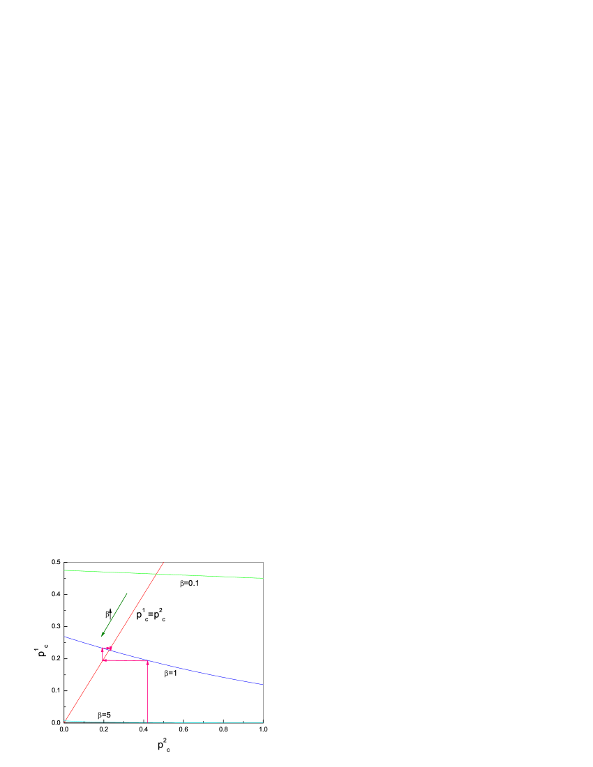
Figure 1: The iteration process defined by the Kinetics Equation of Prisoner’s Dilemma drives the fixed point from a finite number to 0 when $\beta$ growths. Because here only one parameter $p_{c}$ we need to calculate, a simple fixed point graph shows the result. Usually in a multi-strategy game or with more players, we will have more parameters and more complex equations. Then in that situation, we will have to use simulation. The function plotted here is $p_{c}=\frac{1}{1+e^{\beta\left(1+p_{c}\right)}}$. Because the two steps of one iteration use the same function form, it can be regarded as two iteration steps with only one function.

Second example, we choose Hawk-Dove, a two-pure-NE game. The payoff matrix of player $1$ and $2$ are

$$H^{1}=\left[\begin{array}[]{cccc}3&0&0&0\\ 0&1&0&0\\ 0&0&4&0\\ 0&0&0&0\end{array}\right],H^{2}=\left[\begin{array}[]{cccc}3&0&0&0\\ 0&4&0&0\\ 0&0&1&0\\ 0&0&0&0\end{array}\right]$$

The reduced payoff matrix is

$$H^{i}_{R}=\left[\begin{array}[]{cc}3p^{\left(3-i\right)}_{h}+1p^{\left(3-i\right)}_{d}&0\\ 0&4p^{\left(3-i\right)}_{h}\end{array}\right]$$

Then the Kinetics Equation is

$$p^{i}_{h}=\frac{1}{1+e^{\beta\left(p^{\left(3-i\right)}_{h}-p^{\left(3-i\right)}_{d}\right)}}$$

It’s easy to know that when $\beta=\infty$, fixed point are $\left(p^{1}_{h}=0,p^{2}_{h}=1\right)$, $\left(p^{1}_{h}=\frac{1}{2},p^{2}_{h}=\frac{1}{2}\right)$ and $\left(p^{1}_{h}=1,p^{2}_{h}=0\right)$ depending the initial state $p^{2}_{h}>p^{2}_{d}$, $p^{2}_{h}=p^{2}_{d}$ or $p^{2}_{h}<p^{2}_{d}$. For a finite $\beta$, a fixed point graph is shown in fig(2).

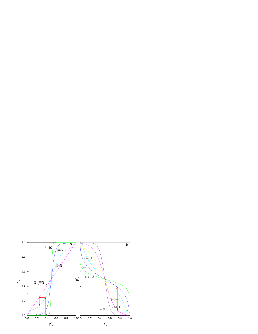
Figure 2: In figure (a), the function plotted is $p_{h}=\frac{1}{1+e^{\beta\left(2\frac{1}{1+e^{\beta\left(2p_{h}-1\right)}}-1\right)}}$. There are three fixed points for this iteration process. One is unstable fixed point, $0.5$, while the other two are stable fixed points closing to $0$ and $1$ respectively, when $\beta$ grows. In figure (b), we explicitly show the two iterations instead of the self-mapping from $p^{1}_{h}$ to $p^{1}_{h}$ in figure (a). It gives more details. $\left(0.5,0.5\right)$ is still an unstable fixed point. While the end state can be a $\left(0,1\right)$ or $\left(1,0\right)$ depending on the initial state.

The third example is the classical penny flip game, which has no pure NE. The payoff matrix are

$$H^{1}=\left[\begin{array}[]{cccc}1&0&0&0\\ 0&-1&0&0\\ 0&0&-1&0\\ 0&0&0&1\end{array}\right]=-H^{2}.$$

The reduced payoff matrix is

$$H^{1}_{R}=\left[\begin{array}[]{cc}p^{2}_{n}-p^{2}_{f}&0\\ 0&p^{2}_{f}-p^{2}_{n}\end{array}\right],H^{2}_{R}=\left[\begin{array}[]{cc}p^{1}_{f}-p^{1}_{n}&0\\ 0&p^{1}_{n}-p^{1}_{f}\end{array}\right].$$

Then the Kinetics Equation is

$$p^{1}_{n}=\frac{1}{1+e^{2\beta\left(p^{2}_{f}-p^{2}_{n}\right)}},p^{2}_{n}=\frac{1}{1+e^{2\beta\left(p^{1}_{n}-p^{1}_{f}\right)}}.$$

From fig(3), $\left(p^{1}_{n}=\frac{1}{2},p^{2}_{n}=\frac{1}{2}\right)$ is the only fixed point no matter $\beta=\infty$ or not. And even the only fixed point is unstable.

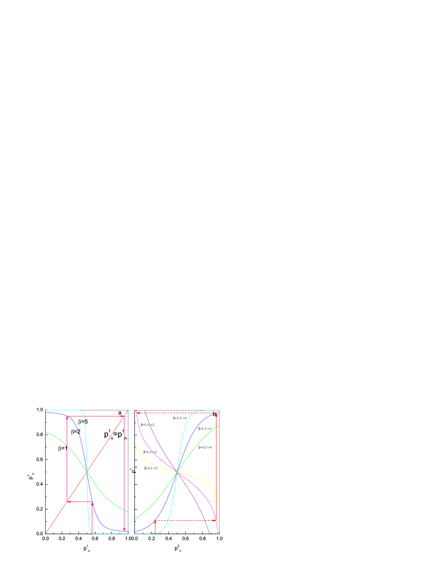
Figure 3: In figure (a), the function plotted here is $p^{1}_{n}=\frac{1}{1+e^{2\beta\left(1-2\frac{1}{1+2\beta\left(2p^{1}_{n}-1\right)}\right)}}$. The only fixed but unstable point is always $0.5$ for different $\beta$. In figure (b), two iteration functions are used to show a clearer but more complex picture, from which we know $\left(0.5,0.5\right)$ is still a fixed point, but if starts from initial state other than this point, the system will jump between $\left(0,0\right)$, $\left(0,1\right)$, $\left(1,1\right)$ and $\left(1,0\right)$.

The Kinetics Equation, its fixed points and the stability analysis of the fixed points gives a method to find equilibrium state and to refine them if we require an applicable equilibrium point is a stable fixed point. From all the trivial cases we tested it seems valid. But questions such as more tests, a general form of such equation, and the relation between such fixed points and Nash Equilibrium is waiting for more detailed discussion.

At last, we have to admit that our simulation is not equivalent with the Kinetics Equation. Pure strategies are included by the Kinetics Equation, but since our algorithm is classical, here we only let it evolute in the subspace of mixture strategy. For classical game, this is not a fatal problem, because we have prove that pure strategy is equivalent with mixture strategy having the same diagonal part. But for a quantum game, pure strategy is totaly different with the mixture classical one because of the off-diagonal elements of payoff matrix. Is it possible to find such a simulation algorithm?

On the other hand, when $\beta\neq\infty$, the fixed point of our Kinetics Equation might not equal to the Nash Equilibrium state. Such fixed points are the end states when the average resolution level of all players is $\beta$, which can be regarded as a typical scale which players care. This concepts may expand the description of Game Theory into the situation that players are not complete rational. They can evaluate the payoff, but not explicitly, only a rough range. And from the experience in Statistical Physics, especially Phase Transition, we know that even when $\beta$ is not very large but large enough the lowest energy mode (here, maximum payoff mode) will dominate the system. This means, under some not extremely restricted conditions, the traditional Nash Equilibrium is still valid. It will be funny if one can prove such conclusion from a general situation in our equilibrium definition.

4 Discussion

It’s quite straightforward to extend our notation into $N$-player game and continuous strategy case. However, although a new representation has been introduced to express everything in a static game, the advantage of such a language and the meaning of all other games is still open. And further more, if it’s acceptable for static game, is it possible to be developed into Evolutionary Game Theory? And cooperative game? Is it related with entangled system state?

As discussed in section 3.2, because of the iteration procedure and the distribution function we used, a natural way of equilibrium calculation and refinement is provided by our pseudo-dynamical method. The non-trivial phase transition happening in Statistical Physics at finite $\beta=\beta_{c}$ implies the probability that when $N>>1$ the traditional equilibrium state can be reached at some finite noise level, not necessary at no-noise infinite-resolution background. In this paper, we only argued such possibility, not by a real example. Further analysis should be done to confirm such statement, although we believe it from the background in Physics.

And as discussed in section 2.4, when our representation is used in Quantum Game Theory, a set of base vectors of strategy (operator) space and their inner product need to be defined to form them as a Hilbert space. Then all the other procedures are quite straightforward. At least, it gives equivalent description. But there are still some open questions, like what’s the meaning of a non-unitary operator in the strategy space? Does physical operator have to be unitary operator? Another interesting question is the effect of base vector transformation of Hilbert space. What happens if base vectors other than our $\left(N^{c},F^{c},N^{q},F^{q}\right)$ are used?

We have to say our present result is a theory far from complete. It stacks in our hands for a very long time, now we want to share the idea with all. In fact, it’s even possible to be nothing than a toy representation of Game Theory. However, even in such case, it’s still of little value to provide a unified description and a possible pseudo-dynamical equation theory which might be completed later so that the end state of iteration from an arbitrary initial will be the Equilibrium State. As you may already noticed our paper is filled with questions other than their answers. Hopefully it will motivate the discussion. Ironically, during the revision of this paper, we found that the idea using a Hilbert space to describe classical and quantum strategies has been proposed in [7] long time before. So our works can be regarded as a realization and development of this idea. In our paper, not only strategies, but also payoff functions has been reexpressed into Hilbert space and operators on it.

5 Conclusions and outlook

Besides lots of questions in above section, here we summarize the reliable conclusions we have till now. First, in the new representation, all games including classical, quantum, even entangled game, under general $N$-player $\left(\prod_{i=1}^{N}L_{i}\right)$ case, can be defined by a unified definition as equ(41). All the difference among the games is at the base vectors of strategy space and the payoff matrix — a $\left(1,1\right)$-tensor. In the traditional form, payoff function of $N$-player classical game is $\left(0,N\right)$-tensor; and for quantum game, it depends on $\mathcal{H}$ and $\rho_{0}$, even not a tensor form. We have to use special language for every specific game.

Second, in our representation, for quantum games, it’s easy to see the role of Off-diagonal elements of payoff matrix when we say a quantum player can make more money over classical player. If the payoff matrix is diagonal, it makes no difference, although a quantum player can make use of quantum pure strategy, which has off-diagonal elements in density matrix. Game Quantum is only possible when both density matrix and payoff matrix have off-diagonal elements. However, unfortunately, as we have pointed out in section $\S\ref{spayoffmatrix}$, quantization of classical game probably changes the definition of original classical game.

Third, with the form of payoff matrix and reduced payoff matrix, equilibrium density matrix in Quantum Statistical Mechanics $e^{\beta H_{R}^{i}}$ gives an equilibrium distribution over strategy space. This provides some flexibility on the application of game theory such as average behavior and collapse into Nash Equilibrium under infinite resolution level ($\beta=\infty$). This helps take partial rationality into our theory. Therefor, for classical game, although our new representation brings nothing new theoretically, it may provide some new technical tools to analyze the NE, to include partial rationality, and to develop evolutionary game.

If such a representation can provide some other insightful advantage besides an equivalent representation of both Classical and Quantum Game Theory, it’s necessary to try more real games, both classical and quantum, in the new framework. From the section $\S$3.2.1, we see that because the system space is the direct space of all players’, the matrix form will be so large that it make all calculations un-convenient. In Quantum Mechanics, the idea to solve such problem is to introduce particle-number representation to replace direct product of base vectors. For undistinguishable particles, such approach significantly reduce the hardwork of calculation. Maybe such simplification can be generalized into Game Theory.

6 Acknowledgement

The author want to thank Dr. Shouyong Pei, Qiang Yuan, Zengru Di, Yougui Wang and Dahui Wang for their inspiring discussion and the great patience to listen to my struggling argument at anytime. Thanks also is given to Prof. Zhanru Yang, Dr. J. Eisert and Dr. L. Marinatto for their suggestions to the revision.

References

- [1] M. J. Osborne and A. Rubinstein, A course in Game Theory, MIT Press, 1994.
- [2] J.W. Friedman, Game Theory with application in Economics, New York: Oxford University Press, 1990.
- [3] E.W. Piotrowski and J. Sladkowski, An invitation to Quantum Game Theory, Int. J. Theor. Phys. 42(2003), 1089.
- [4] A.P. Flitney and D. Abbot, An introduction to quantum game theory, Fluctuation and Noise Letters Vol. 2, No. 4(2002), R175-R187.
- [5] J. Eisert, M. Wilkens, and M. Lewenstein, Quantum Games and Quantum Strategies, Phys. Rev. Lett, 83(1999), 3077.
- [6] D.A. Meyer, Quantum Strategies, Phys. Rev. Lett. 82(1999), 1052.
- [7] L. Marinatto and T. Weber, A quantum approach to static games of complete information, Phys. Lett. A 272(2000), 291.
- [8] M.E.J. Newman and G.T. Barkema, Monte Carlo Method in Statistical Physics, New York: Oxford University Press, 1999.