Adiabatic approximation in open quantum systems

Abstract

We generalize the standard quantum adiabatic approximation to the case of open quantum systems. We define the adiabatic limit of an open quantum system as the regime in which its dynamical superoperator can be decomposed in terms of independently evolving Jordan blocks. We then establish validity and invalidity conditions for this approximation and discuss their applicability to superoperators changing slowly in time. As an example, the adiabatic evolution of a two-level open system is analyzed.

I Introduction

The adiabatic theorem Born:28 ; Kato:50 ; Messiah:book is one of the oldest and most useful general tools in quantum mechanics. The theorem posits, roughly, that if a state is an instantaneous eigenstate of a sufficiently slowly varying Hamiltonian $H$ at one time, then it will remain an eigenstate at later times, while its eigenenergy evolves continuously. Its role in the study of slowly varying quantum mechanical systems spans a vast array of fields and applications, such as energy-level crossings in molecules Landau:32 ; Zener:32 , quantum field theory Gellmann:51 , and geometric phases Berry:84 ; Wilczek:84 . In recent years, geometric phases have been proposed to perform quantum information processing ZanardiRasseti:99 ; ZanardiRasseti:2000 ; Ekert-Nature , with adiabaticity assumed in a number of schemes for geometric quantum computation (e.g., Pachos:00 ; Duan-Science:01 ; Pachos:02 ; Fazio:03 ). Moreover, additional interest in adiabatic processes has arisen in connection with the concept of adiabatic quantum computing, in which slowly varying Hamiltonians appear as a promising mechanism for the design of new quantum algorithms and even as an alternative to the conventional quantum circuit model of quantum computation Farhi:00 ; Farhi:01 .

Remarkably, the notion of adiabaticity does not appear to have been extended in a systematic manner to the arena of open quantum systems, i.e., quantum systems coupled to an external environment Breuer:book . Such systems are of fundamental interest, as the notion of a closed system is always an idealization and approximation. This issue is particularly important in the context of quantum information processing, where environment-induced decoherence is viewed as a fundamental obstacle on the path to the construction of quantum information processors (e.g., LidarWhaley:03 ).

The aim of this work is to systematically generalize the concept of adiabatic evolution to the realm of open quantum systems. Formally, an open quantum system is described as follows. Consider a quantum system $S$ coupled to an environment, or bath $B$ (with respective Hilbert spaces $\mathcal{H}_{S},\mathcal{H}_{B}$), evolving unitarily under the total system-bath Hamiltonian $H_{SB}$. The exact system dynamics is given by tracing over the bath degrees of freedom Breuer:book

$$\rho(t)=\mathrm{Tr}_{B}[U(t)\rho_{SB}(0)U^{{\dagger}}(t)],$$ (1)

where $\rho(t)$ is the system state, $\rho_{SB}(0)=\rho(0)\otimes\rho_{B}(0)$ is the initially uncorrelated system-bath state, and $U(t)=\mathcal{T}\mathsf{\exp}[-i\int_{0}^{t}H_{SB}(t^{\prime})dt^{\prime}]$ ($\mathcal{T}$ denotes time-ordering; we set $\hbar=1$). Such an evolution is completely positive and trace preserving Breuer:book ; Kraus:71 ; Alicki:87 . Under certain approximations, it is possible to convert Eq. (1) into the convolutionless form

$${\dot{\rho}}(t) = \mathcal{L}(t)\rho(t).$$ (2)

An important example is

$${\dot{\rho}}(t) = -i\left[H(t),\rho(t)\right]+\frac{1}{2}\sum_{i=1}^{N}\left([\Gamma_{i}(t),\rho(t)\Gamma^{\dagger}_{i}(t)]\right.$$ (3)

$$\left.+[\Gamma_{i}(t)\rho(t),\Gamma^{\dagger}_{i}(t)]\right).$$

Here $H(t)$ is the time-dependent effective Hamiltonian of the open system and $\Gamma_{i}(t)$ are time-dependent operators describing the system-bath interaction. In the literature, Eq. (3) with time-independent operators $\Gamma_{i}$ is usually referred to as the Markovian dynamical semigroup, or Lindblad equation Breuer:book ; Alicki:87 ; Gorini:76 ; Lindblad:76 [see also Ref. Lidar:CP01 for a simple derivation of Eq. (3) from Eq. (1)]. However, the case with time-dependent coefficients is also permissible under certain restrictions Lendi:86 . The Lindblad equation requires the assumption of a Markovian bath with vanishing correlation time. Equation (2) can be more general; for example, it applies to the case of non-Markovian convolutionless master equations studied in Ref. Breuer:04 . In this work we will consider the class of convolutionless master equations (2). In a slight abuse of nomenclature, we will henceforth refer to the time-dependent generator $\mathcal{L}(t)$ as the Lindblad superoperator, and the $\Gamma_{i}(t)$ as Lindblad operators.

Returning to the problem of adiabatic evolution, conceptually, the difficulty in the transition from closed to open systems is that the notion of Hamiltonian eigenstates is lost, since the Lindblad superoperator – the generalization of the Hamiltonian – cannot in general be diagonalized. It is then not a priori clear what should take the place of the adiabatic eigenstates. Our key insight in resolving this difficulty is that this role is played by adiabatic Jordan blocks of the Lindblad superoperator. The Jordan canonical form Horn:book , with its associated left and right eigenvectors, is in this context the natural generalization of the diagonalization of the Hamiltonian. Specifically, we show that, for slowly varying Lindblad superoperators, the time evolution of the density matrix, written in a suitable basis in the state space of linear operators, occurs separately in sets of Jordan blocks related to each Lindblad eigenvalue. This treatment for adiabatic processes in open systems is potentially rather attractive as it can simplify the description of the dynamical problem by breaking down the Lindblad superoperator into a set of decoupled blocks. In order to clearly exemplify this behavior, we analyze a simple two-level open system for which the exact solution of the master equation (2) can be analytically determined.

The paper is organized as follows. We begin, in Sec. II, with a review of the standard adiabatic approximation for closed quantum systems. In Sec. III we describe the general dynamics of open quantum systems, review the superoperator formalism, and introduce a strategy to find suitable bases in the state space of linear operators. Section IV is devoted to deriving our adiabatic approximation, including the conditions for its validity. In Sec. V, we provide a concrete example which illustrates the consequences of the adiabatic behavior for systems in the presence of decoherence. Finally, we present our conclusions in Sec. VI.

II The adiabatic approximation in closed quantum systems

II.1 Condition on the Hamiltonian

To facilitate comparison with our later derivation of the adiabatic approximation for open systems, let us begin by reviewing the adiabatic approximation in closed quantum systems, subject to unitary evolution. In this case, the evolution is governed by the time-dependent Schrödinger equation

$$H(t)\,|\psi(t)\rangle=i\,|{\dot{\psi}}(t)\rangle,$$ (4)

where $H(t)$ denotes the Hamiltonian and $|\psi(t)\rangle$ is a quantum state in a $D$-dimensional Hilbert space. For simplicity, we assume that the spectrum of $H(t)$ is entirely discrete and nondegenerate. Thus we can define an instantaneous basis of eigenenergies by

$$H(t)\,|n(t)\rangle=E_{n}(t)\,|n(t)\rangle,$$ (5)

with the set of eigenvectors $|n(t)\rangle$ chosen to be orthonormal. In this simplest case, where to each energy level there corresponds a unique eigenstate, adiabaticity is then defined as the regime associated to an independent evolution of the instantaneous eigenvectors of $H(t)$. This means that instantaneous eigenstates at one time evolve continuously to the corresponding eigenstates at later times, and that their corresponding eigenenergies do not cross. In particular, if the system begins its evolution in a particular eigenstate $|n(0)\rangle$, then it will evolve to the instantaneous eigenstate $|n(t)\rangle$ at a later time $t$, without any transition to other energy levels. In order to obtain a general validity condition for adiabatic behavior, let us expand $|\psi(t)\rangle$ in terms of the basis of instantaneous eigenvectors of $H(t)$,

$$|\psi(t)\rangle=\sum_{n=1}^{D}a_{n}(t)\,e^{-i\int_{0}^{t}dt^{\prime}E_{n}(t^{\prime})}\,|n(t)\rangle,$$ (6)

with $a_{n}(t)$ being complex functions of time. Substitution of Eq. (6) into Eq. (4) yields

$$\sum_{n}\left({\dot{a}}_{n}|n\rangle+a_{n}|{\dot{n}}\rangle\right)\,e^{-i\int_{0}^{t}dt^{\prime}E_{n}(t^{\prime})}=0,$$ (7)

where use has been made of Eq. (5). Multiplying Eq. (7) by $\langle k(t)|$, we have

$${\dot{a}}_{k}=-\sum_{n}a_{n}\langle k|{\dot{n}}\rangle\,e^{-i\int_{0}^{t}dt^{\prime}g_{nk}(t^{\prime})},$$ (8)

where

$$g_{nk}(t)\equiv E_{n}(t)-E_{k}(t).$$ (9)

A useful expression for $\langle k|{\dot{n}}\rangle$, for $k\neq n$, can be found by taking the time derivative of Eq. (5) and multiplying the resulting expression by $\langle k|$, which reads

$$\langle k|{\dot{n}}\rangle=\frac{\langle k|{\dot{H}}|n\rangle}{g_{nk}}\quad(n\neq k).$$ (10)

Therefore, Eq. (8) can be written as

$${\dot{a}}_{k}=-a_{k}\langle k|{\dot{k}}\rangle-\sum_{n\neq k}a_{n}\frac{\langle k|{\dot{H}}|n\rangle}{g_{nk}}\,e^{-i\int_{0}^{t}dt^{\prime}g_{nk}(t^{\prime})}.$$ (11)

Adiabatic evolution is ensured if the coefficients $a_{k}(t)$ evolve independently from each other, i.e., if their dynamical equations do not couple. As is apparent from Eq. (11), this requirement is fulfilled by imposing the conditions

$$\max_{0\leq t\leq T}\left|\frac{\langle k|{\dot{H}}|n\rangle}{g_{nk}}\right|\,\ll\,\min_{0\leq t\leq T}\left|{g_{nk}}\right|,$$ (12)

which serves as an estimate of the validity of the adiabatic approximation, where $T$ is the total evolution time. Note that the left-hand side of Eq. (12) has dimensions of frequency and hence must be compared to the relevant physical frequency scale, given by the gap $g_{nk}$ Messiah:book ; Mostafazadeh:book . For a discussion of the adiabatic regime when there is no gap in the energy spectrum see Refs. Avron:98 ; Avron:99 . In the case of a degenerate spectrum of $H(t)$, Eq. (10) holds only for eigenstates $|k\rangle$ and $|n\rangle$ for which $E_{n}\neq E_{k}$. Taking into account this modification in Eq. (11), it is not difficult to see that the adiabatic approximation generalizes to the statement that each degenerate eigenspace of $H(t)$, instead of individual eigenvectors, has independent evolution, whose validity conditions given by Eq. (12) are to be considered over eigenvectors with distinct energies. Thus, in general one can define adiabatic dynamics of closed quantum systems as follows:

Definition II.1

A closed quantum system is said to undergo adiabatic dynamics if its Hilbert space can be decomposed into decoupled Schrödinger eigenspaces with distinct, time-continuous, and noncrossing instantaneous eigenvalues of $H(t)$.

It is conceptually useful to point out that the relationship between slowly varying Hamiltonians and adiabatic behavior, which explicitly appears from Eq. (12), can also be demonstrated directly from a simple manipulation of the Schrödinger equation: recall that $H(t)$ can be diagonalized by a unitary similarity tranformation

$$H_{d}(t)=U^{-1}(t)\,H(t)\,U(t),$$ (13)

where $H_{d}(t)$ denotes the diagonalized Hamiltonian and $U(t)$ is a unitary transformation. Multiplying Eq. (4) by $U^{-1}(t)$ and using Eq. (13), we obtain

$$H_{d}\,|\psi\rangle_{d}=i\,|{\dot{\psi}}\rangle_{d}-i\,{\dot{U}}^{-1}|\psi\rangle,$$ (14)

where $|\psi\rangle_{d}\equiv U^{-1}|\psi\rangle$ is the state of the system in the basis of eigenvectors of $H(t)$. Upon considering that $H(t)$ changes slowly in time, i.e., $dH(t)/dt\approx 0$, we may also assume that the unitary transformation $U(t)$ and its inverse $U^{-1}(t)$ are slowly varying operators, yielding

$$H_{d}(t)\,|\psi(t)\rangle_{d}=i\,|{\dot{\psi}}(t)\rangle_{d}.$$ (15)

Thus, since $H_{d}(t)$ is diagonal, the system evolves separately in each energy sector, ensuring the validity of the adiabatic approximation. In our derivation of the condition of adiabatic behavior for open systems below, we will make use of this semi-intuitive picture in order to motivate the decomposition of the dynamics into Lindblad-Jordan blocks.

II.2 Condition on the total evolution time

The adiabaticity condition can also be given in terms of the total evolution time $T$. We shall consider for simplicity a nondegenerate $H(t)$; the generalization to the degenerate case is possible. Let us then rewrite Eq. (11) as follows Gottfried:book :

$$e^{i\gamma_{k}(t)}\,\frac{\partial}{\partial t}[a_{k}(t)\,e^{-i\gamma_{k}(t)}]=-\sum_{n\neq k}a_{n}\frac{\langle k|{\dot{H}}|n\rangle}{g_{nk}}\,e^{-i\int_{0}^{t}dt^{\prime}g_{nk}(t^{\prime})},$$ (16)

where $\gamma_{k}(t)$ denotes the Berry’s phase Berry:84 associated to the state $|k\rangle$,

$$\gamma_{k}(t)=i\int_{0}^{t}dt^{\prime}\langle k(t^{\prime})|{\dot{k}}(t^{\prime})\rangle.$$ (17)

Now let us define a normalized time $s$ through the variable transformation

$$t=sT,\,\,\,\,\,0\leq s\leq 1.$$ (18)

Then, by performing the change $t\rightarrow s$ in Eq. (16) and integrating, we obtain

$$a_{k}(s)\,e^{-i\gamma_{k}(s)}=$$

$$a_{k}(0)-\sum_{n\neq k}\int_{0}^{s}ds^{\prime}\frac{F_{nk}(s^{\prime})}{g_{nk}(s^{\prime})}e^{-iT\int_{0}^{s^{\prime}}ds^{\prime\prime}g_{nk}(s^{\prime\prime})},$$ (19)

where

$$F_{nk}(s)=a_{n}(s)\,\langle k(s)|\frac{dH(s)}{ds}|n(s)\rangle\,e^{-i\gamma_{k}(s)}.$$ (20)

However, for an adiabatic evolution as defined above, the coefficients $a_{n}(s)$ evolve without any mixing, which means that $a_{n}(s)\approx a_{n}(0)\,e^{i\gamma_{n}(s)}$. Therefore,

$$F_{nk}(s)=a_{n}(0)\,\langle k(s)|\frac{dH(s)}{ds}|n(s)\rangle\,e^{-i[\gamma_{k}(s)-\gamma_{n}(s)]}.$$ (21)

In order to arrive at a condition on $T$, it is useful to separate out the fast oscillatory part from Eq. (19). Thus, the integrand in Eq. (19) can be rewritten as

$$\frac{F_{nk}(s^{\prime})}{g_{nk}(s^{\prime})}e^{-iT\int_{0}^{s^{\prime}}ds^{\prime\prime}g_{nk}(s^{\prime\prime})}=$$

$$\frac{i}{T}\left[\frac{d}{ds^{\prime}}\left(\frac{F_{nk}(s^{\prime})}{g_{nk}^{2}(s^{\prime})}e^{-iT\int_{0}^{s^{\prime}}ds^{\prime\prime}g_{nk}(s^{\prime\prime})}\right)\right.$$

$$\left.-\,e^{-iT\int_{0}^{s^{\prime}}ds^{\prime\prime}g_{nk}(s^{\prime\prime})}\frac{d}{ds^{\prime}}\left(\frac{F_{nk}(s^{\prime})}{g_{nk}^{2}(s^{\prime})}\right)\right].$$ (22)

Substitution of Eq. (22) into Eq. (19) results in

$$a_{k}(s)\,e^{-i\gamma_{k}(s)}=$$

$$a_{k}(0)+\frac{i}{T}\sum_{n\neq k}\left(\frac{F_{nk}(0)}{g_{nk}^{2}(0)}-\frac{F_{nk}(s)}{g_{nk}^{2}(s)}e^{-iT\int_{0}^{s}ds^{\prime}g_{nk}(s^{\prime})}\right.$$

$$\left.+\,\int_{0}^{s}ds^{\prime}\,e^{-iT\int_{0}^{s^{\prime}}ds^{\prime\prime}g_{nk}(s^{\prime\prime})}\frac{d}{ds^{\prime}}\frac{F_{nk}(s^{\prime})}{g_{nk}^{2}(s^{\prime})}\right).$$ (23)

A condition for the adiabatic regime can be obtained from Eq. (23) if the integral in the last line vanishes for large $T$. Let us assume that, as $T\rightarrow\infty$, the energy difference remains nonvanishing. We further assume that $d\{F_{nk}(s^{\prime})/g_{nk}^{2}(s^{\prime})\}/ds^{\prime}$ is integrable on the interval $\left[0,s\right]$. Then it follows from the Riemann-Lebesgue lemma Churchill:book that the integral in the last line of Eq. (23) vanishes in the limit $T\rightarrow\infty$ (due to the fast oscillation of the integrand) RiemannLebesgue . What is left are therefore only the first two terms in the sum over $n\neq k$ of Eq. (23). Thus, a general estimate of the time rate at which the adiabatic regime is approached can be expressed by

$$T\gg\frac{F}{g^{2}},$$ (24)

where

$$F=\max_{0\leq s\leq 1}|a_{n}(0)\,\langle k(s)|\frac{dH(s)}{ds}|n(s)\rangle|,$$

$$g=\min_{0\leq s\leq 1}|g_{nk}(s)|\,,$$ (25)

with $\max$ and $\min$ taken over all $k$ and $n$. A simplification is obtained if the system starts its evolution in a particular eigenstate of $H(t)$. Taking the initial state as the eigenvector $|m(0)\rangle$, with $a_{m}(0)=1$, adiabatic evolution occurs if

$$T\gg\frac{\mathcal{F}}{\mathcal{G}^{2}},$$ (26)

where

$$\mathcal{F}=\max_{0\leq s\leq 1}|\langle k(s)|\frac{dH(s)}{ds}|m(s)\rangle|\,,$$

$$\mathcal{G}=\min_{0\leq s\leq 1}|g_{mk}(s)|\,.$$ (27)

Equation (26) gives an important validity condition for the adiabatic approximation, which has been used, e.g., to determine the running time required by adiabatic quantum algorithms Farhi:00 ; Farhi:01 .

III The dynamics of open quantum systems

In this section, we prepare the mathematical framework required to derive an adiabatic approximation for open quantum systems. Our starting point is the convolutionless master equation (2). It proves convenient to transform to the superoperator formalism, wherein the density matrix is represented by a $D^{2}$-dimensional “coherence vector”

$$|\rho\rangle\rangle=\left(\begin{array}[]{cccc}\rho_{1}&\rho_{2}&\cdots&\rho_{D^{2}}\end{array}\right)^{t},$$ (28)

and the Lindblad superoperator $\mathcal{L}$ becomes a $(D^{2}\times D^{2})$-dimensional supermatrix Alicki:87 . We use the double bracket notation to indicate that we are not working in the standard Hilbert space of state vectors. Such a representation can be generated, e.g., by introducing a basis of Hermitian, trace-orthogonal, and traceless operators [e.g., su($D$)], whence the $\rho_{i}$ are the expansion coefficients of $\rho$ in this basis Alicki:87 , with $\rho_{1}$ the coefficient of $I$ (the identity matrix). In this case, the condition $\mathrm{Tr}\rho^{2}\leq 1$ corresponds to $\left\||\rho\rangle\rangle\right\|\leq 1$, $\rho=\rho^{{\dagger}}$ to $\rho_{i}=\rho_{i}^{\ast}$, and positive semidefiniteness of $\rho$ is expressed in terms of inequalities satisfied by certain Casimir invariants [e.g., of $su(D)$] byrd:062322 ; Kimura:2003-1 ; Kimura:2003-2 . A simple and well-known example of this procedure is the representation of the density operator of a two-level system (qubit) on the Bloch sphere, via $\rho=(I_{2}+\overrightarrow{v}\cdot\overrightarrow{\sigma})/2$, where $\overrightarrow{\sigma}=(\sigma_{x},\sigma_{y},\sigma_{z})$ is the vector of Pauli matrices, $I_{2}$ is the $2\times 2$ identity matrix, and $\overrightarrow{v}\in\mathbb{R}^{3}$ is a three-dimensional coherence vector of norm$\leq 1$. More generally, coherence vectors live in Hilbert-Schmidt space: a state space of linear operators endowed with an inner product that can be defined, for general vectors $u$ and $v$, as

$$(u,v)\equiv\langle\langle u|v\rangle\rangle\equiv\frac{1}{{\mathcal{N}}}{\text{Tr}}\left(u^{\dagger}v\right),$$ (29)

where ${\mathcal{N}}$ is a normalization factor. Adjoint elements $\langle\langle v|$ in the dual state space are given by row vectors defined as the transpose conjugate of $|v\rangle\rangle$: $\langle\langle v|=(v_{1}^{\ast},v_{2}^{\ast},...,v_{D^{2}}^{\ast})$. A density matrix can then be expressed as a discrete superposition of states over a complete basis in this vector space, with appropriate constraints on the coefficients so that the requirements of Hermiticity, positive semidefiniteness, and unit trace of $\rho$ are observed. Thus, representing the density operator in general as a coherence vector, we can rewrite Eq. (2) in a superoperator language as

$$\mathcal{L}(t)\,|\rho(t)\rangle\rangle=|{\dot{\rho}}(t)\rangle\rangle,$$ (30)

where $\mathcal{L}$ is now a supermatrix. This master equation generates nonunitary evolution, since $\mathcal{L}(t)$ is non-Hermitian and hence generally nondiagonalizable. However, it is always possible to obtain an elegant decomposition in terms of a block structure, the Jordan canonical form Horn:book . This can be achieved by the similarity transformation

$$\mathcal{L}_{J}(t)=S^{-1}(t)\,\mathcal{L}(t)\,S(t),$$ (31)

where $\mathcal{L}_{J}(t)=\mathrm{diag}(J_{1},...,J_{m})$ denotes the Jordan form of $\mathcal{L}(t)$, with $J_{\alpha}$ representing a Jordan block related to an eigenvector whose corresponding eigenvalue is $\lambda_{\alpha}$,

$$J_{\alpha}=\left(\begin{array}[]{ccccc}\lambda_{\alpha}&1&0&\cdots&0\\ 0&\lambda_{\alpha}&1&\cdots&0\\ \vdots&\ddots&\ddots&\ddots&\vdots\\ 0&\cdots&0&\lambda_{\alpha}&1\\ 0&\cdots&\cdots&0&\lambda_{\alpha}\end{array}\right).$$ (32)

The number $m$ of Jordan blocks is given by the number of linearly independent eigenstates of $\mathcal{L}(t)$, with each eigenstate associated to a different block $J_{\alpha}$. Since $\mathcal{L}(t)$ is in general non-Hermitian, we generally do not have a basis of eigenstates, whence some care is required in order to find a basis for describing the density operator. A systematic procedure for finding a convenient discrete vector basis is to start from the instantaneous right and left eigenstates of $\mathcal{L}(t)$, which are defined by

$$\mathcal{L}(t)\,|\mathcal{P}_{\alpha}(t)\rangle\rangle = \lambda_{\alpha}(t)\,|\mathcal{P}_{\alpha}(t)\rangle\rangle,$$ (33)

$$\langle\langle Q_{\alpha}(t)|\,\mathcal{L}(t) = \langle\langle Q_{\alpha}(t)|\,\lambda_{\alpha}(t),$$ (34)

where, in our notation, possible degeneracies correspond to $\lambda_{\alpha}=\lambda_{\beta}$, with $\alpha\neq\beta$. In other words, we reserve a different index $\alpha$ for each independent eigenvector since each eigenvector is in a distinct Jordan block. It can immediately be shown from Eqs. (33) and (34) that, for $\lambda_{\alpha}\neq\lambda_{\beta}$, we have $\langle\langle Q_{\alpha}(t)|\mathcal{P}_{\beta}(t)\rangle\rangle=0$. The left and right eigenstates can be easily identified when the Lindblad superoperator is in the Jordan form $\mathcal{L}_{J}(t)$. Denoting $|\mathcal{P}_{\alpha}(t)\rangle\rangle_{J}=S^{-1}(t)\,|\mathcal{P}_{\alpha}(t)\rangle\rangle$, i.e., the right eigenstate of $\mathcal{L}_{J}(t)$ associated to a Jordan block $J_{\alpha}$, then Eq. (33) implies that $|\mathcal{P}_{\alpha}(t)\rangle\rangle_{J}$ is time-independent and, after normalization, is given by

$$\left.|\mathcal{P}_{\alpha}\rangle\rangle_{J}\frac{{}}{{}}\right|_{J_{\alpha}}=\left(\begin{array}[]{c}1\\ 0\\ \vdots\\ 0\\ \end{array}\right),$$ (35)

where only the vector components associated to the Jordan block $J_{\alpha}$ are shown, with all the others vanishing. In order to have a complete basis we shall define new states, which will be chosen so that they preserve the block structure of $\mathcal{L}_{J}(t)$. A suitable set of additional vectors is

$$\left.|\mathcal{D}_{\alpha}^{(1)}\rangle\rangle_{J}\frac{{}}{{}}\right|_{J_{\alpha}}=\left(\begin{array}[]{c}0\\ 1\\ 0\\ \vdots\\ 0\\ \end{array}\right),\,...\,,\,\left.|\mathcal{D}_{\alpha}^{(n_{\alpha}-1)}\rangle\rangle_{J}\frac{{}}{{}}\right|_{J_{\alpha}}=\left(\begin{array}[]{c}0\\ 0\\ 0\\ \vdots\\ 1\\ \end{array}\right),$$ (36)

where $n_{\alpha}$ is the dimension of the Jordan block $J_{\alpha}$ and again all the components outside $J_{\alpha}$ are zero. This simple vector structure allows for the derivation of the expression

$$\mathcal{L}_{J}(t)\,|\mathcal{D}_{\alpha}^{(j)}\rangle\rangle_{J}=|\mathcal{D}_{\alpha}^{(j-1)}\rangle\rangle_{J}+\lambda_{\alpha}(t)\,|\mathcal{D}_{\alpha}^{(j)}\rangle\rangle_{J},$$ (37)

with $|\mathcal{D}_{\alpha}^{(0)}\rangle\rangle_{J}\equiv|\mathcal{P}_{\alpha}\rangle\rangle_{J}$ and  $|\mathcal{D}_{\alpha}^{(-1)}\rangle\rangle_{J}\equiv 0$. The set $\left\{|\mathcal{D}_{\alpha}^{(j)}\rangle\rangle_{J},\text{\thinspace with}\,j=0,...,(n_{\alpha}-1)\right\}$ can immediately be related to a right vector basis for the original $\mathcal{L}(t)$ by means of the transformation $|\mathcal{D}_{\alpha}^{(j)}(t)\rangle\rangle=S(t)\,|\mathcal{D}_{\alpha}^{(j)}\rangle\rangle_{J}$ which, applied to Eq. (37), yields

$$\mathcal{L}(t)\,|\mathcal{D}_{\alpha}^{(j)}(t)\rangle\rangle=|\mathcal{D}_{\alpha}^{(j-1)}(t)\rangle\rangle+\lambda_{\alpha}(t)\,|\mathcal{D}_{\alpha}^{(j)}(t)\rangle\rangle.$$ (38)

Equation (38) exhibits an important feature of the set $\left\{|\mathcal{D}_{\beta}^{(j)}(t)\rangle\rangle\right\}$, namely, it implies that Jordan blocks are invariant under the action of the Lindblad superoperator. An analogous procedure can be employed to define the left eigenbasis. Denoting by ${}_{J}\langle\langle\mathcal{Q}_{\alpha}(t)|=\langle\langle\mathcal{Q}_{\alpha}(t)|S(t)$ the left eigenstate of $\mathcal{L}_{J}(t)$ associated to a Jordan block $J_{\alpha}$, Eq. (34) leads to the normalized left vector

$$\left.{}_{J}\langle\langle\mathcal{Q}_{\alpha}|\frac{{}}{{}}\right|_{J_{\alpha}}=\left(\frac{{}}{{}}0,\,.\,.\,.\,,0,1\frac{{}}{{}}\right).$$ (39)

The additional left vectors are defined as

$$\left.{}_{J}\langle\langle\mathcal{E}_{\alpha}^{(0)}|\frac{{}}{{}}\right|_{J_{\alpha}} = \left(\frac{{}}{{}}1,0,0,\,.\,.\,.\,,0\frac{{}}{{}}\right),$$

$$.\,\,.\,\,.$$

$$\vspace{0.1cm}\left.{}_{J}\langle\langle\mathcal{E}_{\alpha}^{(n_{\alpha}-2)}|\frac{{}}{{}}\right|_{J_{\alpha}} = \left(\frac{{}}{{}}0,\,.\,.\,.\,,0,1,0\frac{{}}{{}}\right),$$ (40)

which imply the following expression for the left basis vector $\langle\langle\mathcal{E}_{\alpha}^{(i)}(t)|=\,_{J}\langle\langle\mathcal{E}_{\alpha}^{(i)}|\,S^{-1}(t)$ for $\mathcal{L}(t)$:

$$\langle\langle\mathcal{E}_{\alpha}^{(i)}(t)|\,\mathcal{L}(t)=\langle\langle\mathcal{E}_{\alpha}^{(i+1)}(t)|+\langle\langle\mathcal{E}_{\alpha}^{(i)}(t)|\,\lambda_{\alpha}(t).$$ (41)

Here we have used the notation ${}_{J}\langle\langle\mathcal{E}_{\alpha}^{(n_{\alpha}-1)}|\equiv\,_{J}\langle\langle\mathcal{Q}_{\alpha}|$ and ${}_{J}\langle\langle\mathcal{E}_{\alpha}^{(n_{\alpha})}|\equiv 0$. A further property following from the definition of the right and left vector bases introduced here is

$$\langle\langle\mathcal{E}_{\alpha}^{(i)}(t)|\mathcal{D}_{\beta}^{(j)}(t)\rangle\rangle=\,_{J}\langle\langle\mathcal{E}_{\alpha}^{(i)}|\mathcal{D}_{\beta}^{(j)}\rangle\rangle_{J}=\delta_{\alpha\beta}\delta^{ij}.$$ (42)

This orthonormality relationship between corresponding left and right states will be very useful in our derivation below of the conditions for the validity of the adiabatic approximation.

IV The adiabatic approximation in open quantum systems

We are now ready to derive our main result: an adiabatic approximation for open quantum systems. We do this by observing that the Jordan decomposition of $\mathcal{L}(t)$ [Eq. (31)] allows for a nice generalization of the standard quantum adiabatic approximation. We begin by defining the adiabatic dynamics of an open system as a generalization of the definition given above for closed quantum systems:

Definition IV.1

An open quantum system is said to undergo adiabatic dynamics if its Hilbert-Schmidt space can be decomposed into decoupled Lindblad–Jordan eigenspaces with distinct, time-continuous, and noncrossing instantaneous eigenvalues of $\mathcal{L}(t)$.

This definition is a natural extension for open systems of the idea of adiabatic behavior. Indeed, in this case the master equation (2) can be decomposed into sectors with different and separately evolving Lindblad-Jordan eigenvalues, and we show below that the condition for this to occur is appropriate “slowness” of the Lindblad superoperator. The splitting into Jordan blocks of the Lindblad superoperator is achieved through the choice of a basis which preserves the Jordan block structure as, for example, the sets of right $\left\{|\mathcal{D}_{\beta}^{(j)}(t)\rangle\rangle\right\}$ and left $\left\{\langle\langle\mathcal{E}_{\alpha}^{(i)}(t)|\right\}$ vectors introduced in Sec. III. Such a basis generalizes the notion of Schrödinger eigenvectors.

IV.1 Intuitive derivation

Let us first show how the adiabatic Lindblad-Jordan blocks arise from a simple argument, analogous to the one presented for the closed case [Eqs. (13)-(15)]. Multiplying Eq. (30) by the similarity transformation matrix $S^{-1}(t)$, we obtain

$$\mathcal{L}_{J}\,|\rho\rangle\rangle_{J}=|{\dot{\rho}}\rangle\rangle_{J}-{\dot{S}}^{-1}\,|\rho\rangle\rangle,$$ (43)

where we have used Eq. (31) and defined $|\rho\rangle\rangle_{J}\equiv S^{-1}|\rho\rangle\rangle$. Now suppose that $\mathcal{L}(t)$, and consequently $S(t)$ and its inverse $S^{-1}(t)$, changes slowly in time so that ${\dot{S}}^{-1}(t)\approx 0$. Then, from Eq. (43), the adiabatic dynamics of the system reads

$$\mathcal{L}_{J}(t)\,|\rho(t)\rangle\rangle_{J}=|{\dot{\rho}}(t)\rangle\rangle_{J}.$$ (44)

Equation (44) ensures that, choosing an instantaneous basis for the density operator $\rho(t)$ which preserves the Jordan block structure, the evolution of $\rho(t)$ occurs separately in adiabatic blocks associated with distinct eigenvalues of $\mathcal{L}(t)$. Of course, the conditions under which the approximation ${\dot{S}}^{-1}(t)\approx 0$ holds must be carefully clarified. This is the subject of the next two subsections.

IV.2 Condition on the Lindblad superoperator

Let us now derive the validity conditions for open-system adiabatic dynamics by analyzing the general time evolution of a density operator under the master equation (30). To this end, we expand the density matrix for an arbitrary time $t$ in the instantaneous right eigenbasis $\left\{|{\mathcal{D}_{\beta}^{(j)}(t)\rangle\rangle}\right\}$ as

$$|\rho(t)\rangle\rangle=\frac{1}{2}\sum_{\beta=1}^{m}\sum_{j=0}^{n_{\beta}-1}r_{\beta}^{(j)}(t)\,|\mathcal{D}_{\beta}^{(j)}(t)\rangle\rangle,$$ (45)

where $m$ is the number of Jordan blocks and $n_{\beta}$ is the dimension of the block $J_{\beta}$. We emphasize that we are assuming that there are no eigenvalue crossings in the spectrum of the Lindblad superoperator during the evolution. Requiring then that the density operator Eq. (45) evolves under the master equation (30) and making use of Eq. (38), we obtain

$$\sum_{\beta=1}^{m}\sum_{j=1}^{n_{\beta}-1}r_{\beta}^{(j)}\,\left(|\mathcal{D}_{\beta}^{(j-1)}\rangle\rangle+\lambda_{\beta}\,|\mathcal{D}_{\beta}^{(j)}\rangle\rangle\right)=$$

$$\sum_{\beta=1}^{m}\sum_{j=0}^{n_{\beta}-1}\left({\dot{r}}_{\beta}^{(j)}\,|\mathcal{D}_{\beta}^{(j)}\rangle\rangle+r_{\beta}^{(j)}\,|{\dot{\mathcal{D}}}_{\beta}^{(j)}\rangle\rangle\right).$$ (46)

Equation (46) multiplied by the left eigenstate $\langle\langle\mathcal{E}_{\alpha}^{(i)}|$ results in

$${\dot{r}}_{\alpha}^{(i)}=\lambda_{\alpha}\,r_{\alpha}^{(i)}+r_{\alpha}^{(i+1)}-\sum_{\beta=1}^{m}\sum_{j=0}^{n_{\beta}-1}r_{\beta}^{(j)}\langle\langle\mathcal{E}_{\alpha}^{(i)}|{\dot{\mathcal{D}}}_{\beta}^{(j)}\rangle\rangle,$$ (47)

with $r_{\alpha}^{(n_{\alpha})}(t)\equiv 0$. Note that the sum over $\beta$ mixes different Jordan blocks. An analogous situation occurred in the closed system case, in Eq. (11). Similarly to what was done there, in order to derive an adiabaticity condition we must separate this sum into terms related to the eigenvalue $\lambda_{\alpha}$ of $\mathcal{L}(t)$ and terms involving mixing with eigenvalues $\lambda_{\beta}\neq\lambda_{\alpha}$. In this latter case, an expression can be found for $\langle\langle\mathcal{E}_{\alpha}^{(i)}|{\dot{\mathcal{D}}}_{\beta}^{(j)}\rangle\rangle$ as follows: taking the time derivative of Eq. (38) and multiplying by $\langle\langle\mathcal{E}_{\alpha}^{(i)}|$ we obtain, after using Eqs. (41) and (42),

$$\langle\langle\mathcal{E}_{\alpha}^{(i)}|{\dot{\mathcal{D}}}_{\beta}^{(j)}\rangle\rangle=\frac{1}{\omega_{\beta\alpha}}\,\left(\,\langle\langle\mathcal{E}_{\alpha}^{(i)}|\,{\dot{\mathcal{L}}}\,|\mathcal{D}_{\beta}^{(j)}\rangle\rangle\,\right.$$

$$\left.+\,\langle\langle\mathcal{E}_{\alpha}^{(i+1)}|{\dot{\mathcal{D}}}_{\beta}^{(j)}\rangle\rangle-\langle\langle\mathcal{E}_{\alpha}^{(i)}|{\dot{\mathcal{D}}}_{\beta}^{(j-1)}\rangle\rangle\,\right),\,\,\,\,$$ (48)

where we have defined

$$\omega_{\beta\alpha}(t)\equiv\lambda_{\beta}(t)-\lambda_{\alpha}(t)$$ (49)

and assumed $\lambda_{\alpha}\neq\lambda_{\beta}$. Note that, while $\omega_{\beta\alpha}$ plays a role analogous to that of the energy difference $g_{nk}$ in the closed case [Eq. (9)], $\omega_{\beta\alpha}$ may be complex. A similar procedure can generate expressions for all the terms $\langle\langle\mathcal{E}_{\alpha}^{(i)}|{\dot{\mathcal{D}}}_{\beta}^{(j-k)}\rangle\rangle$, with $k=0,...,j$. Thus, an iteration of Eq. (48) yields

$$\langle\langle\mathcal{E}_{\alpha}^{(i)}|{\dot{\mathcal{D}}}_{\beta}^{(j)}\rangle\rangle = \sum_{k=0}^{j}\frac{(-1)^{k}}{\omega_{\beta\alpha}^{k+1}}\left(\langle\langle\mathcal{E}_{\alpha}^{(i)}|\,{\dot{\mathcal{L}}}\,|\mathcal{D}_{\beta}^{(j-k)}\rangle\rangle\,\right.$$ (50)

$$\left.+\,\langle\langle\mathcal{E}_{\alpha}^{(i+1)}|{\dot{\mathcal{D}}}_{\beta}^{(j-k)}\rangle\rangle\right).$$

From a second recursive iteration, now for the term $\langle\langle\mathcal{E}_{\alpha}^{(i+1)}|{\dot{\mathcal{D}}}_{\beta}^{(j-k)}\rangle\rangle$ in Eq. (50), we obtain

$$\langle\langle\mathcal{E}_{\alpha}^{(i)}|{\dot{\mathcal{D}}}_{\beta}^{(j)}\rangle\rangle=$$

$$\sum_{p=1}^{(n_{\alpha}-i)}\left(\prod_{q=1}^{p}\sum_{k_{q}=0}^{(j-S_{q-1})}\right)\frac{\langle\langle\mathcal{E}_{\alpha}^{(i+p-1)}|{\dot{\mathcal{L}}}|\mathcal{D}_{\beta}^{(j-S_{p})}\rangle\rangle}{(-1)^{S_{p}}\,\omega_{\beta\alpha}^{p+S_{p}}},$$ (51)

where

$$S_{q}=\sum_{s=1}^{q}k_{s}\,\,\,\,,\,\,\,\,\left(\prod_{q=1}^{p}\sum_{k_{q}=0}^{(j-S_{q-1})}\right)=\sum_{k_{1}=0}^{j-S_{0}}\cdots\sum_{k_{p}=0}^{j-S_{p-1}},$$ (52)

with $S_{0}=0$. We can now split Eq. (47) into diagonal and off-diagonal terms

$${\dot{r}}_{\alpha}^{(i)}=\lambda_{\alpha}r_{\alpha}^{(i)}+r_{\alpha}^{(i+1)}-\sum_{\beta\,|\,\lambda_{\beta}=\lambda_{\alpha}}\sum_{j=0}^{n_{\beta}-1}r_{\beta}^{(j)}\langle\langle\mathcal{E}_{\alpha}^{(i)}|{\dot{\mathcal{D}}}_{\beta}^{(j)}\rangle\rangle\hskip 8.5359pt$$

$$-\sum_{\beta\,|\,\lambda_{\beta}\neq\lambda_{\alpha}}\sum_{j=0}^{n_{\beta}-1}r_{\beta}^{(j)}\langle\langle\mathcal{E}_{\alpha}^{(i)}|{\dot{\mathcal{D}}}_{\beta}^{(j)}\rangle\rangle,$$ (53)

where the terms $\langle\langle\mathcal{E}_{\alpha}^{(i)}|{\dot{\mathcal{D}}}_{\beta}^{(j)}\rangle\rangle$, for $\lambda_{\beta}\neq\lambda_{\alpha}$, are given by Eq. (51). In accordance with our definition of adiabaticity above, the adiabatic regime is obtained when the sum in the second line is negligible. Summarizing, by introducing the normalized time $s$ defined by Eq. (18), we thus find the following from Eqs. (51) and (53).

Theorem IV.2

A sufficient condition for open quantum system adiabatic dynamics as given in Definition IV.1 is:

$$\max_{0\leq s\leq 1}\,\left|\sum_{p=1}^{(n_{\alpha}-i)}\left(\prod_{q=1}^{p}\sum_{k_{q}=0}^{(j-S_{q-1})}\right)\frac{\langle\langle\mathcal{E}_{\alpha}^{(i+p-1)}|\frac{d\mathcal{L}}{ds}|\mathcal{D}_{\beta}^{(j-S_{p})}\rangle\rangle}{(-1)^{S_{p}}\,\omega_{\beta\alpha}^{p+S_{p}}}\right|$$

$$\ll 1,$$ (54)

with $\lambda_{\beta}\neq\lambda_{\alpha}$ and for arbitrary indices $i$ and $j$ associated to the Jordan blocks $\alpha$ and $\beta$, respectively.

The condition (54) ensures the absence of mixing of coefficients $r_{\alpha}^{(i)}$ related to distinct eigenvalues $\lambda_{\alpha}$ in Eq. (53), which in turn guarantees that sets of Jordan blocks belonging to different eigenvalues of $\mathcal{L}(t)$ have independent evolution. Thus the accuracy of the adiabatic approximation can be estimated by the computation of the time derivative of the Lindblad superoperator acting on right and left vectors. Equation (54) can be simplified by considering the term with maximum absolute value, which results in:

Corollary IV.3

A sufficient condition for open quantum system adiabatic dynamics is

$${\cal N}_{ij}^{n_{\alpha}n_{\beta}}\max_{0\leq s\leq 1}\,\left|\frac{\langle\langle\mathcal{E}_{\alpha}^{(i+p-1)}|\frac{d\mathcal{L}}{ds}|\mathcal{D}_{\beta}^{(j-S_{p})}\rangle\rangle}{\omega_{\beta\alpha}^{p+S_{p}}}\right|\ll 1,$$ (55)

where the $\max$ is taken for any $\alpha\neq\beta$, and over all possible values of $i\in\{0,...,n_{\alpha}-1\}$, $j\in\{0,...,n_{\beta}-1\}$, and $p$, with

$${\cal N}_{ij}^{n_{\alpha}n_{\beta}}=\sum_{p=1}^{(n_{\alpha}-i)}\left(\prod_{q=1}^{p}\sum_{k_{q}=0}^{(j-S_{q-1})}\right)1$$ (56)

$$=\left(\begin{array}[c]{c}n_{\alpha}-i+1+j\\ 1+j\end{array}\right)-1=\frac{(n_{\alpha}-i+1+j)!}{(1+j)!(n_{\alpha}-i)!}-1.$$ (59)

Observe that the factor ${\cal N}_{ij}^{n_{\alpha}n_{\beta}}$ defined in Eq. (56) is just the number of terms of the sums in Eq. (54). We have included a superscript $n_{\beta}$, even though there is no explicit dependence on $n_{\beta}$, since $j\in\{0,...,n_{\beta}-1\}$.

Furthermore, an adiabatic condition for a slowly varying Lindblad super-operator can directly be obtained from Eq. (54), yielding the following.

Corollary IV.4

A simple sufficient condition for open quantum system adiabatic dynamics is ${\dot{\mathcal{L}}}\approx 0$.

Note that this condition is in a sense too strong, since it need not be the case that $\dot{\mathcal{L}}$ is small in general (i.e., for all its matrix elements). Indeed, in Sec. V we show via an example that adiabaticity may occur due to the exact vanishing of relevant matrix elements of ${\dot{\mathcal{L}}}$. The general condition for this to occur is the presence of a dynamical symmetry Bohm:88 .

Let us end this subsection by mentioning that we can also write Eq. (54) in terms of the time variable $t$ instead of the normalized time $s$. In this case, the natural generalization of Eq. (54) is

$$\max_{0\leq t\leq T}\,\left|\sum_{p=1}^{(n_{\alpha}-i)}\left(\prod_{q=1}^{p}\sum_{k_{q}=0}^{(j-S_{q-1})}\right)\frac{\langle\langle\mathcal{E}_{\alpha}^{(i+p-1)}|{\dot{\mathcal{L}}}|\mathcal{D}_{\beta}^{(j-S_{p})}\rangle\rangle}{(-1)^{S_{p}}\,\omega_{\beta\alpha}^{p+S_{p}}}\right|$$

$$\ll\,\min_{0\leq t\leq T}\,|\omega_{\beta\alpha}|.$$ (60)

Note that, as in the analogous condition (12) in the closed case, the left-hand side has dimensions of frequency, and hence must be compared to the natural frequency scale $\omega_{\beta\alpha}$. However, unlike the closed systems case, where Eq. (12) can immediately be derived from the time condition (24), we cannot prove here that $\omega_{\beta\alpha}$ is indeed the relevant physical scale. Therefore, Eq. (60) should be regarded as a heuristic criterion.

IV.3 Condition on the total evolution time

As mentioned in Sec. II, for closed systems the rate at which the adiabatic regime is approached can be estimated in terms of the total time of evolution, as shown by Eqs. (24) and (26). We now provide a generalization of this estimate for adiabaticity in open systems.

IV.3.1 One-dimensional Jordan blocks

Let us begin by considering the particular case where $\mathcal{L}(t)$ has only one-dimensional Jordan blocks and each eigenvalue corresponds to a single independent eigenvector, i.e., $\lambda_{\alpha}=\lambda_{\beta}\Rightarrow\alpha=\beta$. Bearing these assumptions in mind, Eq. (53) can be rewritten as

$${\dot{r}}_{\alpha}=\lambda_{\alpha}r_{\alpha}-r_{\alpha}\langle\langle\mathcal{E}_{\alpha}|{\dot{\mathcal{D}}}_{\alpha}\rangle\rangle-\sum_{\beta\neq\alpha}r_{\beta}\langle\langle\mathcal{E}_{\alpha}|{\dot{\mathcal{D}}}_{\beta}\rangle\rangle,$$ (61)

where the upper indices $i,j$ have been removed since we are considering only one-dimensional blocks. Moreover, for this special case, we have from Eq. (51)

$$\langle\langle\mathcal{E}_{\alpha}|{\dot{\mathcal{D}}}_{\beta}\rangle\rangle=\frac{\langle\langle\mathcal{E}_{\alpha}|\,{\dot{\mathcal{L}}}\,|\mathcal{D}_{\beta}\rangle\rangle}{\omega_{\beta\alpha}}.$$ (62)

In order to eliminate the term $\lambda_{\alpha}r_{\alpha}$ from Eq. (61), we redefine the variable $r_{\alpha}(t)$ as

$$r_{\alpha}(t)=p_{\alpha}(t)\,e^{\int_{0}^{t}\lambda_{\alpha}(t^{\prime})dt^{\prime}},$$ (63)

which, applied to Eq. (61), yields

$${\dot{p}}_{\alpha}=-p_{\alpha}\,\langle\langle\mathcal{E}_{\alpha}|{\dot{\mathcal{D}}}_{\alpha}\rangle\rangle-\sum_{\beta\neq\alpha}p_{\beta}\,\langle\langle\mathcal{E}_{\alpha}|{\dot{\mathcal{D}}}_{\beta}\rangle\rangle\,e^{\Omega_{\beta\alpha}},$$ (64)

with

$$\Omega_{\beta\alpha}(t)=\int_{0}^{t}dt^{\prime}\,\omega_{\beta\alpha}(t^{\prime}).$$ (65)

Equation (64) is very similar to Eq. (11) for closed systems, but the fact that $\Omega_{\beta\alpha}$ is in general complex-valued leads to some important differences, discussed below. We next introduce the scaled time $s=t/T$ and integrate the resulting expression. Using Eq. (62), we then obtain

$$p_{\alpha}(s)\,=\,p_{\alpha}(0)-\int_{0}^{s}ds^{\prime}p_{\alpha}(s^{\prime})\,\Phi_{\alpha}(s^{\prime})$$

$$-\sum_{\beta\neq\alpha}\int_{0}^{s}ds^{\prime}\frac{V_{\beta\alpha}(s^{\prime})}{\omega_{\beta\alpha}(s^{\prime})}\,e^{T\,\Omega_{\beta\alpha}(s^{\prime})},$$ (66)

where $\Phi_{\alpha}(s)$ is defined by

$$\Phi_{\alpha}(s)=\langle\langle\mathcal{E_{\alpha}}(s)|\frac{d}{ds}|\mathcal{D_{\alpha}}(s)\rangle\rangle$$ (67)

and $V_{\beta\alpha}(s)$ by

$$V_{\beta\alpha}(s)=p_{\beta}(s)\,\langle\langle\mathcal{E_{\alpha}}(s)|\frac{d\mathcal{L}(s)}{ds}|\mathcal{D_{\beta}}(s)\rangle\rangle.$$ (68)

The integrand in the last line of Eq. (66) can be rearranged in a similar way to Eq. (22) for the closed case, yielding

$$\frac{V_{\beta\alpha}(s)}{\omega_{\beta\alpha}(s)}\,e^{T\,\Omega_{\beta\alpha}(s)}$$ (69)

$$= \frac{1}{T}\left[\frac{d}{ds}\left(\frac{V_{\beta\alpha}}{\omega_{\beta\alpha}^{2}}\,e^{T\,\Omega_{\beta\alpha}(s)}\right)-e^{T\,\Omega_{\beta\alpha}(s)}\frac{d}{ds}\frac{V_{\beta\alpha}}{\omega_{\beta\alpha}^{2}}\right].$$

Therefore, from Eq. (66) we have

$$p_{\alpha}(s)\,=\,p_{\alpha}(0)-\int_{0}^{s}ds^{\prime}p_{\alpha}(s^{\prime})\,\Phi_{\alpha}(s^{\prime})$$

$$+\frac{1}{T}\sum_{\beta\neq\alpha}\left(\frac{V_{\beta\alpha}(0)}{\omega_{\beta\alpha}^{2}(0)}-\frac{V_{\beta\alpha}(s)}{\omega_{\beta\alpha}^{2}(s)}\,e^{T\,\Omega_{\beta\alpha}(s)}\right.$$

$$\left.+\int_{0}^{s}ds^{\prime}\,e^{T\,\Omega_{\beta\alpha}(s^{\prime})}\frac{d}{ds^{\prime}}\frac{V_{\beta\alpha}(s^{\prime})}{\omega_{\beta\alpha}^{2}(s^{\prime})}\right).$$ (70)

Thus a condition for adiabaticity in terms of the total time of evolution can be given by comparing $T$ to the terms involving indices $\beta\neq\alpha$. This can be formalized as follows.

Proposition IV.5

Consider an open quantum system whose Lindblad superoperator $\mathcal{L}(s)$ has the following properties: $(a)$ The Jordan decomposition of $\mathcal{L}(s)$ is given by one-dimensional blocks. $(b)$ Each eigenvalue of $\mathcal{L}(s)$ is associated to a unique Jordan block. Then the adiabatic dynamics in the interval $0\leq s\leq 1$ occurs if and only if the following time conditions, obtained for each Jordan block $\alpha$ of $\mathcal{L}(s)$, are satisfied:

$$T \gg \max_{0\leq s\leq 1}\left|\,\sum_{\beta\neq\alpha}\left(\frac{V_{\beta\alpha}(0)}{\omega_{\beta\alpha}^{2}(0)}-\frac{V_{\beta\alpha}(s)}{\omega_{\beta\alpha}^{2}(s)}\,e^{T\,\Omega_{\beta\alpha}(s)}\right.\right.$$ (71)

$$\left.\left.+\int_{0}^{s}ds^{\prime}\,e^{T\,\Omega_{\beta\alpha}(s^{\prime})}\frac{d}{ds^{\prime}}\frac{V_{\beta\alpha}(s^{\prime})}{\omega_{\beta\alpha}^{2}(s^{\prime})}\right)\right|,$$

Equation (71) simplifies in a number of situations.

• Adiabaticity is guaranteed whenever $V_{\beta\alpha}$ vanishes for all $\alpha\neq\beta$. An example of this case will be provided in Sec. V.

• Adiabaticity is similarly guaranteed whenever $V_{\beta\alpha}(s)$, which can depend on $T$ through $p_{\beta}$, vanishes for all $\alpha,\beta$ such that $\mathrm{Re}(\Omega_{\beta\alpha})>0$ and does not grow faster, as a function of $T$, than $\exp(T|\,{\mathrm{Re}}\Omega_{\beta\alpha}|)$ for all $\alpha,\beta$ such that $\mathrm{Re}(\Omega_{\beta\alpha})<0$.

• When $\mathrm{Re}(\Omega_{\beta\alpha})=0$ and $\mathrm{Im}(\Omega_{\beta\alpha})\neq 0$ the integral in inequality (71) vanishes in the infinite time limit due to the Riemann-Lebesgue lemma Churchill:book , as in the closed case discussed before. In this case, again, adiabaticity is guaranteed provided $p_{\beta}(s)$ [and hence $V_{\beta\alpha}(s)$] does not diverge as a function of $T$ in the limit $T\rightarrow\infty$.

• When $\mathrm{Re}(\Omega_{\beta\alpha})>0$, the adiabatic regime can still be reached for large $T$ provided that $p_{\beta}(s)$ contains a decaying exponential which compensates for the growing exponential due to $\mathrm{Re}(\Omega_{\beta\alpha})$.

• Even if there is an overall growing exponential in inequality (71), adiabaticity could take place over a finite time interval $[0,T_{\ast}]$ and, afterwards, disappear. In this case, which would be an exclusive feature of open systems, the crossover time $T_{\ast}$ would be determined by an inequality of the type $T\gg a+b\exp(cT)$, with $c>0$. The coefficients $a,b$ and $c$ are functions of the system-bath interaction. Whether the latter inequality can be solved clearly depends on the values of $a,b,c$, so that a conclusion about adiabaticity in this case is model dependent.

IV.3.2 General Jordan blocks

We show now that the hypotheses $(a)$ and $(b)$ can be relaxed, providing a generalization of Proposition IV.5 for the case of multidimensional Jordan blocks and Lindblad eigenvalues associated to more than one independent eigenvector. Let us redefine our general coefficient $r_{\alpha}^{(i)}(t)$ as

$$r_{\alpha}^{(i)}(t)=p_{\alpha}^{(i)}(t)\,e^{\int_{0}^{t}\lambda_{\alpha}(t^{\prime})dt^{\prime}},$$ (72)

which, applied to Eq. (53), yields

$${\dot{p}}_{\alpha}^{(i)}\,=\,p_{\alpha}^{(i+1)}$$

$$-\sum_{\beta\,|\,\lambda_{\beta}=\lambda_{\alpha}}\sum_{j=0}^{n_{\beta}-1}p_{\beta}^{(j)}\langle\langle\mathcal{E}_{\alpha}^{(i)}|{\dot{\mathcal{D}}}_{\beta}^{(j)}\rangle\rangle\,e^{\Omega_{\beta\alpha}}$$

$$-\sum_{\beta\,|\,\lambda_{\beta}\neq\lambda_{\alpha}}\sum_{j=0}^{n_{\beta}-1}p_{\beta}^{(j)}\langle\langle\mathcal{E}_{\alpha}^{(i)}|{\dot{\mathcal{D}}}_{\beta}^{(j)}\rangle\rangle\,e^{\Omega_{\beta\alpha}}.$$ (73)

The above equation can be rewritten in terms of the scaled time $s=t/T$. The integration of the resulting expression then reads

$$p_{\alpha}^{(i)}(s)\,=\,p_{\alpha}^{(i)}(0)+T\int_{0}^{s}ds^{\prime}p_{\alpha}^{(i+1)}(s^{\prime})$$

$$-\sum_{\beta\,|\,\lambda_{\beta}=\lambda_{\alpha}}\sum_{j}\int_{0}^{s}ds^{\prime}p_{\beta}^{(j)}(s^{\prime})\,\Phi_{\beta\alpha}^{(ij)}(s^{\prime})\,e^{T\,\Omega_{\beta\alpha}(s^{\prime})}$$

$$-\sum_{\beta\,|\,\lambda_{\beta}\neq\lambda_{\alpha}}\sum_{j,p}\int_{0}^{s}ds^{\prime}\frac{(-1)^{S_{p}}\,V_{\beta\alpha}^{(ijp)}(s^{\prime})}{\omega_{\beta\alpha}^{p+S_{p}}(s^{\prime})}\,e^{T\,\Omega_{\beta\alpha}(s^{\prime})},$$ (74)

where use has been made of Eq. (51), with the sum over $j$ and $p$ in the last line denoting

$$\sum_{j,p}\equiv\sum_{j=0}^{n_{\beta}-1}\sum_{p=1}^{(n_{\alpha}-i)}\left(\prod_{q=1}^{p}\sum_{k_{q}=0}^{(j-S_{q-1})}\right).$$ (75)

The function $\Phi_{\beta\alpha}^{(ij)}(s)$ is defined by

$$\Phi_{\beta\alpha}^{(ij)}(s)=\langle\langle\mathcal{E}_{\alpha}^{(i)}(s)|\frac{d}{ds}|{\mathcal{D}}_{\beta}^{(j)}(s)\rangle\rangle,$$ (76)

and $V_{\beta\alpha}^{(ijp)}(s)$ by

$$V_{\beta\alpha}^{(ijp)}(s)=p_{\beta}^{(j)}(s)\langle\langle\mathcal{E}_{\alpha}^{(i+p-1)}(s)|\frac{d\mathcal{L}(s)}{ds}|\mathcal{D}_{\beta}^{(j-S_{p})}(s)\rangle\rangle.\,$$ (77)

The term $T\int_{0}^{s}ds^{\prime}p_{\alpha}^{(i+1)}(s^{\prime})$ in the first line of Eq. (74), which was absent in the case of one-dimensional Jordan blocks analyzed above, has no effect on adiabaticity, since it does not cause any mixing of Jordan blocks. Therefore, the analysis can proceed very similarly to the case of one-dimensional blocks. Rewriting the integral in the last line of Eq. (74), as we have done in Eqs. (23) and (70), and imposing the absence of mixing of the eigenvalues $\lambda_{\beta}\neq\lambda_{\alpha}$, i.e., the negligibility of the last line of Eq. (74), we find the following general theorem ensuring the adiabatic behavior of an open system.

Theorem IV.6

Consider an open quantum system governed by a Lindblad superoperator $\mathcal{L}(s)$. Then the adiabatic dynamics in the interval $0\leq s\leq 1$ occurs if and only if the following time conditions, obtained for each coefficient $p_{\alpha}^{(i)}(s)$, are satisfied:

$$T \gg \max_{0\leq s\leq 1}\left|\,\sum_{\beta\,|\,\lambda_{\beta}\neq\lambda_{\alpha}}\sum_{j,p}\,(-1)^{S_{p}}\right.$$ (78)

$$\times\left[\frac{V_{\beta\alpha}^{(ijp)}(0)}{\omega_{\beta\alpha}^{p+S_{p}+1}(0)}-\frac{V_{\beta\alpha}^{(ijp)}(s)\,e^{T\,\Omega_{\beta\alpha}(s)}}{\omega_{\beta\alpha}^{p+S_{p}+1}(s)}\right.$$

$$\left.\left.+\int_{0}^{s}ds^{\prime}\,e^{T\,\Omega_{\beta\alpha}(s^{\prime})}\frac{d}{ds^{\prime}}\frac{V_{\beta\alpha}^{(ijp)}(s^{\prime})}{\omega_{\beta\alpha}^{p+S_{p}+1}(s^{\prime})}\right]\right|.$$

Theorem IV.6 provides a very general condition for adiabaticity in open quantum systems. The comments made about simplifying circumstances, in the case of one-dimensional blocks above, hold here as well. Moreover, a simpler sufficient condition can be derived from Eq. (78) by considering the term with maximum absolute value in the sum. This procedure leads to the following corollary:

Corollary IV.7

A sufficient time condition for the adiabatic regime of an open quantum system governed by a Lindblad superoperator $\mathcal{L}(t)$ is

$$T \gg \mathcal{M}_{ij}^{n_{\alpha}n_{\beta}}\,\max_{0\leq s\leq 1}\left|\,\frac{V_{\beta\alpha}^{(ijp)}(0)}{\omega_{\beta\alpha}^{p+S_{p}+1}(0)}-\frac{V_{\beta\alpha}^{(ijp)}(s)\,e^{T\,\Omega_{\beta\alpha}(s)}}{\omega_{\beta\alpha}^{p+S_{p}+1}(s)}\right.$$ (79)

$$\left.+\int_{0}^{s}ds^{\prime}\,e^{T\,\Omega_{\beta\alpha}(s^{\prime})}\frac{d}{ds^{\prime}}\frac{V_{\beta\alpha}^{(ijp)}(s^{\prime})}{\omega_{\beta\alpha}^{p+S_{p}+1}(s^{\prime})}\right|,$$

where $\max$ is taken over all possible values of the indices $\lambda_{\alpha}\neq\lambda_{\beta}$, $i$, $j$, and $p$, with

$$\mathcal{M}_{ij}^{n_{\alpha}n_{\beta}}=\sum_{\beta\,|\,\lambda_{\beta}\neq\lambda_{\alpha}}\sum_{j=0}^{(n_{\beta}-1)}\sum_{p=1}^{(n_{\alpha}-i)}\left(\prod_{q=1}^{p}\sum_{k_{q}=0}^{(j-S_{q-1})}\right)1$$

$$=\Lambda_{\beta\alpha}\left[\frac{(n_{\alpha}+n_{\beta}-i+1)!}{(n_{\alpha}-i+1)!n_{\beta}!}-n_{\beta}-1\right],$$ (80)

where $\Lambda_{\beta\alpha}$ denotes the number of Jordan blocks such that $\lambda_{\alpha}\neq\lambda_{\beta}$.

IV.4 Physical interpretation of the adiabaticity condition

There are various equivalent ways in which to interpret the adiabatic theorem for closed quantum systems Messiah:book . A particularly useful interpretation follows from Eq. (26): the evolution time must be much longer than the ratio of the norm of the time derivative of the Hamiltonian to the square of the spectral gap. In other words, either the Hamiltonian changes slowly, or the spectral gap is large, or both. It is tempting to interpret our results in a similar fashion, which we now do.

The quantity $V_{\beta\alpha}^{(ijp)}$, by Eq. (77), plays the role of the time derivative of the Lindblad superoperator. However, the appearance of $\exp[T\,\mathrm{Re}\,\Omega_{\beta\alpha}(s)]$ in Eq. (78) has no analog in the closed-systems case, because the eigenvalues of the Hamiltonian are real, while in the open-systems case the eigenvalues of the Lindblad superoperator may have imaginary parts. This implies that adiabaticity is a phenomenon which is not guaranteed to happen in open systems even for very slowly varying interactions. Indeed, from Theorems IV.5 and IV.6, possible pictures of such system evolutions include the decoupling of Jordan blocks only over a finite time interval (disappearing afterwards), or even the case of complete absence of decoupling for any time $T$, which implies no adiabatic evolution whatsoever.

The quantity $\omega_{\beta\alpha}$, by Eq. (49), clearly plays the role of the spectral gap in the open-system case. There are two noteworthy differences compared to the closed-system case. First, the $\omega_{\beta\alpha}$ can be complex. This implies that the differences in decay rates, and not just in energies, play a role in determining the relevant gap for open systems. Second, for multidimensional Jordan blocks, the terms $\omega_{\beta\alpha}$ depend on distinct powers for distinct pairs $\beta,\alpha$. Thus certain $\omega_{\beta\alpha}$ (those with the higher exponents) will play a more dominant role than others.

The conditions for adiabaticity are best illustrated further via examples, one of which we provide next.

V Example: The adiabatic evolution of an open quantum two-level system

In order to illustrate the consequences of open quantum system adiabatic dynamics, let us consider a concrete example that is analytically solvable. Suppose a quantum two-level system, with internal Hamiltonian $H=(\omega/2)\,\sigma_{z}$, and described by the master equation (2), is subjected to two sources of decoherence: spontaneous emission $\Gamma_{1}(t)=\epsilon(t)\,\sigma_{-}$ and bit flips $\Gamma_{2}(t)=\gamma(t)\,\sigma_{x}$, where $\sigma_{-}=\sigma_{x}-i\sigma_{y}$ is the lowering operator. Writing the density operator in the basis $\left\{I_{2},\sigma_{x},\sigma_{y},\sigma_{z}\right\}$, i.e., as $\rho=(I_{2}+\overrightarrow{v}\cdot\overrightarrow{\sigma})/2$, Eq. (30) results in

$$|{\dot{\rho}}(t)\rangle\rangle=\frac{1}{2}\left(\begin{array}[]{c}0\\ -\omega v_{y}-2\epsilon^{2}v_{x}\\ \omega v_{x}-2(\gamma^{2}+\epsilon^{2})v_{y}\\ -4\epsilon^{2}-2(\gamma^{2}+2\epsilon^{2})v_{z}\\ \end{array}\right)=\frac{1}{2}\left(\begin{array}[]{c}0\\ {\dot{v}}_{x}\\ {\dot{v}}_{y}\\ {\dot{v}}_{z}\\ \end{array}\right),$$ (81)

where $v_{x}(t)$, $v_{y}(t)$, and $v_{z}(t)$ are real functions providing the coordinates of the quantum state $|\rho(t)\rangle\rangle$ on the Bloch sphere. The Lindblad superoperator is then given by

$$\mathcal{L}(t)=\left(\begin{array}[]{cccc}0&0&0&0\\ 0&-2\,\epsilon^{2}&-\omega&0\\ 0&\omega&-2\epsilon^{2}-2\gamma^{2}&0\\ -4\,\epsilon^{2}&0&0&-4\epsilon^{2}-2\gamma^{2}\end{array}\right).$$ (82)

In order to exhibit an example that has a nontrivial Jordan block structure, we now assume $\gamma^{2}=\omega$ (which can in practice be obtained by measuring the relaxation rate $\gamma$ and correspondingly adjusting the system frequency $\omega$). We then have three different eigenvalues for $\mathcal{L}(t)$,

$$\lambda_{1} = 0,$$

$$\lambda_{2} = -2\epsilon^{2}-\gamma^{2}\text{ }\mathrm{(twofold\,\,degenerate)}$$

$$\lambda_{3} = -4\epsilon^{2}-2\gamma^{2},$$

which are associated with the following three independent (unnormalized) right eigenvectors:

$$|\mathcal{D}_{1}^{(0)}\rangle\rangle=\left(\begin{array}[]{c}f(\gamma,\epsilon)\\ 0\\ 0\\ 1\\ \end{array}\right),|\mathcal{D}_{2}^{(0)}\rangle\rangle=\left(\begin{array}[]{c}0\\ 1\\ 1\\ 0\\ \end{array}\right),|\mathcal{D}_{3}^{(0)}\rangle\rangle=\left(\begin{array}[]{c}0\\ 0\\ 0\\ 1\\ \end{array}\right),$$ (83)

with $f(\gamma,\epsilon)=-1-(\gamma^{2}/2\epsilon^{2})$. Similarly, for the left eigenvectors, we find

$$\langle\langle\mathcal{E}_{1}^{(0)}| = \left(\frac{{}}{{}}1/f(\gamma,\epsilon),0,0,0\frac{{}}{{}}\right),$$

$$\vspace{0.1cm}\langle\langle\mathcal{E}_{2}^{(1)}| = \left(\frac{{}}{{}}0,\gamma^{2},-\gamma^{2},0\frac{{}}{{}}\right),$$

$$\vspace{0.1cm}\langle\langle\mathcal{E}_{3}^{(0)}| = \left(\frac{{}}{{}}-1/f(\gamma,\epsilon),0,0,1\frac{{}}{{}}\right).$$ (84)

The Jordan form of $\mathcal{L}(t)$ can then be written as

$$\mathcal{L}_{J}(t)=\left(\begin{array}[]{cccc}0&0&0&0\\ 0&-2\epsilon^{2}-\gamma^{2}&1&0\\ 0&0&-2\epsilon^{2}-\gamma^{2}&0\\ 0&0&0&-4\epsilon^{2}-2\gamma^{2}\end{array}\right),$$ (85)

(observe the two-dimensional middle Jordan block), with the transformation matrix leading to the Jordan form being

$$S(t)=\left(\begin{array}[]{cccc}f(\gamma,\epsilon)&0&0&0\\ 0&1&\gamma^{-2}&0\\ 0&1&0&0\\ 1&0&0&1\end{array}\right).$$ (86)

Note that, in our example, each eigenvalue of $\mathcal{L}(t)$ is associated to a unique Jordan block, since we do not have more than one independent eigenvector for each $\lambda_{\alpha}$. We then expect that the adiabatic regime will be characterized by an evolution which can be decomposed by single Jordan blocks. In order to show that this is indeed the case, let us construct a right and left basis preserving the block structure. To this end, we need to introduce a right and a left vector for the Jordan block related to the eigenvalue $\lambda_{2}$. As in Eqs. (36) and (40), we define the additional states as

$$|\mathcal{D}_{2}^{(1)}\rangle\rangle_{J}=\left(\begin{array}[]{c}0\\ 0\\ 1\\ 0\\ \end{array}\right),\,\,\,_{J}\langle\langle\mathcal{E}_{2}^{(0)}|=\left(\frac{{}}{{}}0,1,0,0\frac{{}}{{}}\right).$$ (87)

We then obtain, after applying the transformations $|\mathcal{D}_{2}^{(1)}(t)\rangle\rangle=S(t)\,|\mathcal{D}_{2}^{(1)}\rangle\rangle_{J}$ and $\langle\langle\mathcal{E}_{2}^{(0)}(t)|=\,_{J}\langle\langle\mathcal{E}_{2}^{(0)}|\,S^{-1}(t)$, the right and left vectors

$$|\mathcal{D}_{2}^{(1)}\rangle\rangle=\left(\begin{array}[]{c}0\\ \gamma^{-2}\\ 0\\ 0\\ \end{array}\right),\,\,\,\langle\langle\mathcal{E}_{2}^{(0)}|=\left(\frac{{}}{{}}0,0,1,0\frac{{}}{{}}\right).$$ (88)

Expanding the coherence vector in the basis $\left\{|\mathcal{D}_{\alpha}^{(j)}(t)\rangle\rangle\right\}$, as in Eq. (45), the master equation (30) yields

$$f(\gamma,\epsilon)\,{\dot{r}}_{1}^{(0)}+{\dot{f}}(\gamma,\epsilon)\,r_{1}^{(0)}=0,$$

$${\dot{r}}_{2}^{(0)}-2\frac{{\dot{\gamma}}}{\gamma^{3}}r_{2}^{(1)}+\frac{{\dot{r}}_{2}^{(1)}}{\gamma^{2}}=-\left(2\epsilon^{2}+\gamma^{2}\right)r_{2}^{(0)}-2\frac{\epsilon^{2}}{\gamma^{2}}r_{2}^{(1)},$$

$${\dot{r}}_{2}^{(0)}=r_{2}^{(1)}-\left(2\epsilon^{2}+\gamma^{2}\right)r_{2}^{(0)},$$

$${\dot{r}}_{1}^{(0)}+{\dot{r}}_{3}^{(0)}=\left(-4\epsilon^{2}-2\gamma^{2}\right)\,r_{3}^{(0)},$$ (89)

It is immediately apparent from Eq. (89) that the block related to the eigenvalue $\lambda_{2}$ is already decoupled from the rest. On the other hand, by virtue of the last equation, the blocks associated to $\lambda_{1}$ and $\lambda_{3}$ are coupled, implying a mixing in the evolution of the coefficients $r_{1}^{(0)}(t)$ and $r_{3}^{(0)}(t)$. The role of the adiabaticity will then be the suppression of this coupling. We note that in this simple example, the coupling between $r_{1}^{(0)}(t)$ and $r_{3}^{(0)}(t)$ would in fact also be eliminated by imposing the probability conservation condition $\mathrm{Tr}\rho=1$. However, in order to discuss the effects of the adiabatic regime, let us permit a general time evolution of all coefficients (i.e., probability “leakage”) and analyze the adiabatic constraints. The validity condition for adiabatic dynamics, given by Eq. (60), yields

$$\left|\frac{\langle\langle\mathcal{E}_{3}^{(0)}|\,{\dot{\mathcal{L}}}\,|\mathcal{D}_{1}^{(0)}\rangle\rangle}{\lambda_{1}-\lambda_{3}}\right|=\left|\frac{2\gamma^{2}{\dot{\epsilon}}/\epsilon-2\gamma{\dot{\gamma}}}{\gamma^{2}+2\epsilon^{2}}\right|\ll\left|\lambda_{1}-\lambda_{3}\right|.$$ (90)

We first note that we have here the possibility of an adiabatic evolution even without ${\dot{\mathcal{L}}}(t)\approx 0$ in general (i.e., for all its matrix elements). Indeed, solving $\gamma^{2}{\dot{\epsilon}}/\epsilon=\gamma{\dot{\gamma}}$, Eq. (90) implies that independent evolution in Jordan blocks will occur for $\epsilon(t)\propto\gamma(t)$.  Since $f(\gamma,\epsilon)=-1-(\gamma^{2}/2\epsilon^{2})$ is then constant in time, it follows, from Eq. (89), that $r_{1}^{(0)}(t)$ is constant in time, which in turn ensures the decoupling of $r_{1}^{(0)}(t)$ and $r_{3}^{(0)}(t)$. In this case, it is a dynamical symmetry (constancy of the ratio of magnitudes of the spontaneous emission and bit-flip processes), rather than the general slowness of ${\dot{\mathcal{L}}}(t)$, that is responsible for the adiabatic behavior. The same conclusion is also obtained from the adiabatic condition (54). Of course, Eq. (90) is automatically satisfied if $\mathcal{L}(t)$ is slowly varying in time, which means ${\dot{\gamma}}(t)\approx 0$ and ${\dot{\epsilon}}(t)\approx 0$. Assuming this last case, the following solution is found:

$$r_{1}^{(0)}(t)=r_{1}^{(0)}(0),$$

$$r_{2}^{(0)}(t)=\left[r_{2}^{(1)}(0)\,t+r_{2}^{(0)}(0)\right]\,{e}^{(-2\epsilon^{2}-\gamma^{2})\,t},$$

$$r_{2}^{(1)}(t)=r_{2}^{(1)}(0)\,{e}^{(-2\epsilon^{2}-\gamma^{2})\,t},$$

$$r_{3}^{(0)}(t)=r_{3}^{(0)}(0)\,{e}^{(-4\epsilon^{2}-2\gamma^{2})\,t}.$$ (91)

It is clear that the evolution is independent in the three distinct Jordan blocks, with functions $r_{\alpha}^{(i)}(t)$ belonging to different sectors evolving separately. The only mixing is between $r_{2}^{(0)}(t)$ and $r_{2}^{(1)}(t)$, which are components of the the same block. The decoupling of the coefficients $r_{1}^{(0)}(t)$ and $r_{3}^{(0)}(t)$ in the adiabatic limit is exhibited in Fig. 1. Observe that the adiabatic behavior is recovered as the dependence of $\epsilon(t)$ and $\gamma(t)$ on $t$ becomes negligible.

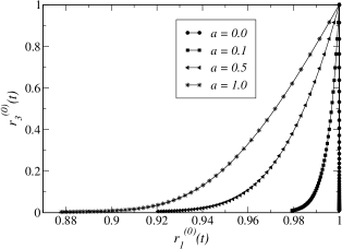
Figure 1: Parametric evolution of the coefficients $r_{3}^{(0)}(t)$ and $r_{1}^{(0)}(t)$ for $0\leq t\leq 1$. The initial conditions are $r_{1}^{(0)}(0)=r_{3}^{(0)}(0)=1.0$ and the decoherence parameters are taken as linear functions of time, i.e., $\epsilon(t)=\epsilon_{0}+at$ and $\gamma(t)=\gamma_{0}+at$, with $\epsilon_{0}=1.0$ and $\gamma_{0}=0.5$. The master equation is solved numerically for $a>0$. In the adiabatic regime, corresponding to $a=0$, the evolution of $r_{1}^{(0)}(t)$ and $r_{3}^{(0)}(t)$ is decoupled, with $r_{1}^{(0)}(t)=1$ independently of the value of $r_{3}^{(0)}(t)$.

The original coefficients $v_{x}$, $v_{y}$, and $v_{z}$ in the Bloch sphere basis $\left\{I_{2},\sigma_{x},\sigma_{y},\sigma_{z}\right\}$ can be written as combinations of the functions $r_{\alpha}^{(i)}$. Equation (91) yields

$$v_{x}(t) = \left(v_{x}(0)+(v_{x}(0)-v_{y}(0))\gamma^{2}\,t\right)\,e^{(-2\epsilon^{2}-\gamma^{2})\,t},$$

$$v_{y}(t) = \left(v_{y}(0)+(v_{x}(0)-v_{y}(0))\gamma^{2}\,t\right)\,e^{(-2\epsilon^{2}-\gamma^{2})\,t},$$

$$v_{z}(t) = \left(v_{z}(0)-\frac{1}{f(\gamma,\epsilon)}\right)e^{(-4\epsilon^{2}-2\gamma^{2})\,t}+\frac{1}{f(\gamma,\epsilon)}$$ (92)

with the initial conditions

$$v_{x}(0)=r_{2}^{(0)}(0)+\gamma^{-2}r_{2}^{(1)}(0),$$

$$v_{y}(0)=r_{2}^{(0)}(0),$$

$$v_{z}(0)=\frac{1}{f(\gamma,\epsilon)}+r_{3}^{(0)}(0),$$ (93)

where now $r_{1}^{(0)}(0)=1/f(\gamma,\epsilon)$ has been imposed in order to satisfy the $\mathrm{Tr}\rho=1$ normalization condition. The Bloch sphere is then characterized by an asymptotic decay of the Bloch coordinates $v_{x}$ and $v_{y}$, with $v_{z}$ approaching the constant value $1/f(\gamma,\epsilon)$.

Finally, let us comment on the analysis of adiabaticity in terms of the conditions derived in Sec. IV.3 for the total time of evolution. Looking at the matrix elements of ${\dot{\cal L}}(t)$, it can be shown that, for $\beta\neq\alpha$, the only term $V_{\beta\alpha}^{(ijp)}$ defined by Eq. (77) which can be a priori nonvanishing is $V_{13}$. Therefore, we have to consider the energy difference $\omega_{13}=4\epsilon^{2}+2\gamma^{2}$. Assuming that the decoherence parameters $\epsilon$ and $\gamma$ are nonvanishing, we have $\omega_{13}>0$ and hence $\Omega_{13}>0$. This signals the breakdown of adiabaticity, unless $V_{13}=0$. However, as we saw above, $V_{13}\propto\langle\langle\mathcal{E}_{3}^{(0)}|\,{\dot{\mathcal{L}}}\,|\mathcal{D}_{1}^{(0)}\rangle\rangle=2\gamma^{2}{\dot{\epsilon}}/\epsilon-2\gamma{\dot{\gamma}}$ and thus $V_{13}=0$ indeed implies the adiabaticity condition $\epsilon(t)\propto\gamma(t)$, in agreement with the results obtained from Theorem IV.2. In this (dynamical symmetry) case adiabaticity holds exactly, while if $\epsilon(t)$ is not proportional to $\gamma(t)$, then there can be no adiabatic evolution. Thus, the present example, despite nicely illustrating our concept of adiabaticity in open systems, does not present us with the opportunity to derive a nontrivial condition on $T$; such more general examples will be discussed in a future publication.

VI Conclusions and outlook

The concept of adiabatic dynamics is one of the pillars of the theory of closed quantum systems. Here we have introduced its generalization to open quantum systems. We have shown that under appropriate slowness conditions the time-dependent Lindblad superoperator decomposes into dynamically decoupled Jordan blocks, which are preserved under the adiabatic dynamics. Our key results are summarized in Theorems IV.2 and IV.6, which state sufficient (and necessary in the case of Theorem IV.6) conditions for adiabaticity in open quantum systems. In particular, Theorem IV.6 also provides the condition for breakdown of the adiabatic evolution. This feature has no analog in the more restricted case of closed quantum systems. It follows here from the fact that the Jordan eigenvalues of the dynamical superoperator – the generalization of the real eigenvalues of a Hamiltonian – can have an imaginary part, which can lead to unavoidable transitions between Jordan blocks. It is worth mentioning that all of our results have been derived considering systems exhibiting gaps in the Lindblad eigenvalue spectrum. It would be interesting to understand the notion of adiabaticity when no gaps are available, as similarly done for the closed case in Refs. Avron:98 ; Avron:99 . Moreover, two particularly intriguing applications of the theory presented here are to the study of geometric phases in open systems and to quantum adiabatic algorithms, both of which have received considerable recent attention Farhi:00 ; Farhi:01 ; Thomaz:03 ; Carollo:04 ; Sanders:04 . We leave these as open problems for future research.

- (1) M. Born and V. Fock, Z. Phys. 51, 165 (1928).
- (2) T. Kato, J. Phys. Soc. Jpn. 5, 435 (1950).
- (3) A. Messiah, Quantum Mechanics (North-Holland, Amsterdam, 1962), Vol. 2.
- (4) L. D. Landau, Zeitschrift 2, 46 (1932).
- (5) C. Zener, Proc. R. Soc. London Ser. A 137, 696 (1932).
- (6) M. Gell-Mann and F. Low, Phys. Rev. 84, 350 (1951).
- (7) M. V. Berry, Proc. R. Soc. London 392, 45 (1989).
- (8) F. Wilczek and A. Zee, Phys. Rev. Lett. 52, 2111 (1984).
- (9) P. Zanardi and M. Rasetti, Phys. Lett. A 264, 94 (1999).
- (10) J. Pachos, P. Zanardi, and M. Rasetti, Phys. Rev. A 61, 010305 (2000).
- (11) J. A. Jones, V. Vedral, A. Ekert, and G. Castagnoli, Nature (London) 403, 869 (2000).
- (12) J. Pachos and S. Chountasis, Phys. Rev. A 62, 052318 (2000).
- (13) L.-M. Duan, J. I. Cirac, and P. Zoller, Science 292, 1695 (2001).
- (14) I. Fuentes-Guridi, J. Pachos, S. Bose, V. Vedral, and S. Choi, Phys. Rev. A 66, 022102 (2002).
- (15) L. Faoro, J. Siewert, and R. Fazio, Phys. Rev. Lett. 90, 028301 (2003).
- (16) E. Farhi, J. Goldstone, S. Gutmann, and M. Sipser, e-print quant-ph/0001106.
- (17) E. Farhi, J. Goldstone, S. Gutmann, J. Lapan, A. Lundgren, and D. Preda, Science 292, 472 (2001).
- (18) H.-P. Breuer and F. Petruccione, The Theory of Open Quantum Systems (Oxford University Press, Oxford, 2002).
- (19) D.A. Lidar and K.B. Whaley, in Irreversible Quantum Dynamics, Vol. 622 of Lecture Notes in Physics, edited by F. Benatti and R. Floreanini (Springer, Berlin, 2003), p. 83 [e-print quant-ph/0301032 (2003)].
- (20) K. Kraus, Ann. Phys. (N.Y.) 64, 311 (1971).
- (21) R. Alicki and K. Lendi, Quantum Dynamical Semigroups and Applications, No. 286 in Lecture Notes in Physics (Springer-Verlag, Berlin, 1987).
- (22) V. Gorini, A. Kossakowski, and E. C. G. Sudarshan, J. Math. Phys. 17, 821 (1976).
- (23) G. Lindblad, Commun. Math. Phys. 48, 119 (1976).
- (24) D.A. Lidar, Z. Bihary, and K.B. Whaley, Chem. Phys. 268, 35 (2001).
- (25) K. Lendi, Phys. Rev. A 33, 3358 (1986).
- (26) H.-P. Breuer, Phys. Rev. A 70, 012106 (2004).
- (27) R. A. Horn and C. R. Johnson, Matrix Analysis (Cambridge University Press, Cambridge, UK, 1999).
- (28) A. Mostafazadeh, Dynamical Invariants, Adiabatic Approximation, and the Geometric Phase (Nova Science Publishers, New York, 2001).
- (29) J. E. Avron and A. Elgart, Phys. Rev. A 58, 4300 (1998).
- (30) J. E. Avron and A. Elgart, Commun. Math. Phys. 203, 445 (1999).
- (31) K. Gottfried and T.-M. Yan, Quantum Mechanics: Fundamentals (Springer, New York, 2003).
- (32) J. W. Brown and R. V. Churchill, Fourier Series and Boundary Value Problems (McGraw-Hill, New York, 1993).
- (33) The Riemann-Lebesgue lemma can be stated through the following proposition: Let be an integrable function on the interval . Then as .
- (34) M. S. Byrd and N. Khaneja, Phys. Rev. A 68, 062322 (2003).
- (35) G. Kimura, Phys. Lett. A 314, 339 (2003).
- (36) G. Kimura, J. Phys. Soc. Jpn. Suppl. C 72, 185 (2003).
- (37) A. Bohm, Y. Ne’eman, and A.O. Barut, Dynamical Groups and Spectrum Generating Algebras: Vol. I (World Scientific, Singapore, 1988).
- (38) A. C. A. Pinto and M. T. Thomaz, J. Phys. A 36, 7461 (2003).
- (39) A. Carollo, I. Fuentes-Guridi, M. F. Santos, and V. Vedral, Phys. Rev. Lett. 92, 020402 (2004).
- (40) I. Kamleitner, J. D. Cresser, and B. C. Sanders, Phys. Rev. A 70, 044103 (2004).