Entangling two mode thermal fields through quantum erasing

Abstract

We investigate a possible scheme for entangling two mode thermal fields through the quantum erasing process, in which an atom is coupled with two mode fields via the interaction governed by the two-mode two-photon Jaynes-Cummings model. The influence of phase decoherence on the entanglement of two mode fields is discussed. It is found that quantum erasing process can transfer part of entanglement between the atom and fields to two mode fields initially in the thermal states. The entanglement achieved by fields heavily depends on their initial temperature and the detuning. The entanglement of stationary state is also investigated.

PACS numbers: 03.67.Mn, 03.67.-a, 03.65.Fd

I. INTRODUCTION

Entanglement, an important resource for quantum information processing [1], is one of the most prominent nonclassical properties in quantum theory. Entanglement can exhibit a nonlocal correlation between quantum systems that have no classical interpretation. Recently, much attention has been focused on the entanglement in bipartite or multipartite systems in which the subsystems are initially in thermal equilibrium [2,3,4,5]. Arnesen et al. have shown that a natural entanglement arises in Heisenberg spin chain in thermal equilibrium, and the entanglement can be improved by increasing the temperature [2]. Instead of attempting to shield the system from the environmental noise, Plenio and Huelge [3] use white noise to play a constructive role and generate the controllable entanglement by incoherent sources. Similar work on this aspect has also been considered by other authors [4,5]. However, very little attention has been paid to the study of entangling two mode thermal fields. In this paper, we investigate a possible scheme for entangling two mode thermal fields through the quantum erasing process, in which an atom is coupled with two mode fields via the interaction governed by the two-mode two-photon Jaynes-Cummings model. The influence of phase decoherence on the entanglement of two mode fields is discussed. It is found that quantum erasing process can transfer part of entanglement between the atom and fields to two mode fields initially in the thermal states. The entanglement achieved by fields heavily depends on their initial temperature and the detuning. The term ”quantum eraser” [6] was invented to describe the loss or gain of interference or, more generally quantum information, in a subensemble, based on the measurement outcomes of two complementary observables. It was reported that the implementation of two- and three-spin quantum eraser using nuclear magnetic resonance, and shown that quantum erasers provide a means of manipulating quantum entanglement [7]. The quantum erasing process discussed in this paper is implemented by measuring the polarizing vector of a two-level atom coupling with two mode quantum fields. The project measurement of an atom has been extensively studied both in the theoretical and experimental aspects.
This paper is organized as follows. In Sec.II, we study the system in which an atom is coupled with two mode fields via the interaction governed by the two-mode two-photon Jaynes-Cummings model by making use of the dynamical algebraical method [8,9] and find the exact solution of the master equation for the system with phase decoherence. Based on the exact solution, we then propose a possible way to entangle two mode thermal fields through the quantum erasing process, which is realized by measuring the atom. In Sec.III, we use the log-negativity to characterize the entanglement between two mode fields. It is shown that quantum erasing process can transfer part of entanglement between the atom and fields to two mode fields initially in the thermal states. The entanglement achieved by fields heavily depends on their initial temperature and the detuning. A conclusion is given in Sec.IV.

II. SOLUTION OF AN ATOM COUPLES TO TWO THERMAL FIELDS WITH PHASE DECOHERENCE

We consider the two-mode two-photon Jaynes-Cummings model [10]. The Hamiltonian for the model can be described by ($\hbar=1$),

$$H=\omega_{1}a^{\dagger}_{1}a_{1}+\omega_{2}a^{\dagger}_{2}a_{2}+\frac{\omega}{2}\sigma_{z}+g(a_{1}a_{2}\sigma_{+}+a^{\dagger}_{1}a^{\dagger}_{2}\sigma_{-}),$$

where $\sigma_{z}$ and $\sigma_{\pm}$ are the atomic spin flip operators characterizing the effective two-level atom with transition frequency $\omega$ and $a_{1}$ ($a_{2}$), $a^{\dagger}_{1}$ ($a^{\dagger}_{2}$) are annihilation and creation operators of the first (second) mode light field of frequencies $\omega_{1}$ ($\omega_{2}$) respectively. The Hamiltonian (1) ignores Stark shifts and the parameter $g$ is the atom-field coupling constant.

It is easy to see that there exist two constants of motion in the Hamiltonian (1),

$$K_{1}=a^{\dagger}_{1}a_{1}+\frac{1+\sigma_{z}}{2},~{}~{}~{}K_{2}=a^{\dagger}_{2}a_{2}+\frac{1+\sigma_{z}}{2},$$

which commute not only with Hamiltonian but also with operators $a_{1}a_{2}\sigma_{+}$ and $a^{\dagger}_{1}a^{\dagger}_{2}\sigma_{-}$. We can introduce the following operators

$$S_{0}=\frac{\sigma_{z}}{2},~{}~{}~{}S_{+}=\frac{a_{1}a_{2}\sigma_{+}}{\sqrt{K_{1}K_{2}}},~{}~{}~{}S_{-}=\frac{a^{\dagger}_{1}a^{\dagger}_{2}\sigma_{-}}{\sqrt{K_{1}K_{2}}}.$$

The operators $S_{\pm}$ and $S_{0}$ satisfy the following commutation relations

$$[S_{0},S_{\pm}]=\pm{S}_{\pm},~{}~{}~{}[S_{+},S_{-}]=2S_{0},$$

where $S_{\pm}$ and $S_{0}$ are the generators of the su(2) algebra. In terms of the su(2) generators, we can rewrite the Hamiltonian (1) as

$$H=\omega_{1}(K_{1}-\frac{1}{2})+\omega_{2}(K_{2}-\frac{1}{2})+\Delta{S}_{0}+g\sqrt{K_{1}K_{2}}(S_{+}+S_{-}),$$

where $\Delta=\omega-\omega_{1}-\omega_{2}$. With the help of the su(2) dynamical algebraic structure, we can diagonalize the Hamiltonian (5) by introducing a unitary transformation

$$U=\exp[\frac{\theta(K_{1},K_{2})}{2}(S_{+}-S_{-})]$$

with $\theta(K_{1},K_{2})=\arctan(2g\sqrt{K_{1}K_{2}}/\Delta)$, and get transformed Hamiltonian

$$H^{\prime}=UHU^{\dagger}=\omega_{1}(K_{1}-\frac{1}{2})+\omega_{2}(K_{2}-\frac{1}{2})+2\Omega(K_{1},K_{2})S_{0},$$

where $\Omega(K_{1},K_{2})=\sqrt{\Delta^{2}/4+g^{2}K_{1}K_{2}}$.

In this paper, we consider the phase decoherence mechanism only. In this situation, the master equation governing the time evolution for the system under the Markovian approximation is given by [11]

$$\frac{d\rho}{dt}=-i[H,\rho]-\frac{\gamma}{2}[H,[H,\rho]],$$

where $\gamma$ is the phase decoherence coefficient. Noted that the equation with the similar form has been proposed to describing the intrinsic decoherence [12]. The formal solution of the master equation (8) can be expressed as follows [13],

$$\rho(t)=\sum^{\infty}_{k=0}\frac{(\gamma{t})^{k}}{k!}M^{k}(t)\rho(0)M^{\dagger{k}}(t),$$

where $\rho(0)$ is the density operators of the initial atom-field system and $M^{k}(t)$ is defined by

$$M^{k}(t)=H^{k}\exp(-iHt)\exp(-\frac{\gamma{t}}{2}H^{2}).$$

By means of the SU(2) dynamical algebraic structure, we obtain the explicit expression for the operator $M^{k}$

$$M^{k}(t)=U^{\dagger}H^{\prime{k}}\exp(-iH^{\prime}t)\exp(-\frac{\gamma{t}}{2}H^{\prime 2})U$$

$$~{}~{}~{}=\frac{1}{2}[\hat{f}^{k}_{+}\exp(-i\hat{f}_{+}t)\exp(-\frac{\gamma{t}\hat{f}^{2}_{+}}{2})+\hat{f}^{k}_{-}\exp(-i\hat{f}_{-}t)\exp(-\frac{\gamma{t}\hat{f}^{2}_{-}}{2})]$$

$$~{}~{}~{}+\frac{1}{2}[\hat{f}^{k}_{+}\exp(-i\hat{f}_{+}t)\exp(-\frac{\gamma{t}\hat{f}^{2}_{+}}{2})-\hat{f}^{k}_{-}\exp(-i\hat{f}_{-}t)\exp(-\frac{\gamma{t}\hat{f}^{2}_{-}}{2})][\frac{\Delta\sigma_{z}}{2\Omega(K_{1},K_{2})}+\frac{g(a_{1}a_{2}\sigma_{+}+a^{\dagger}_{1}a^{\dagger}_{2}\sigma_{-})}{\Omega(K_{1},K_{2})}],$$

where $\hat{f}_{\pm}=\omega_{1}(K_{1}-1/2)+\omega_{2}(K_{2}-1/2)\pm\Omega(K_{1},K_{2})$. Firstly, we assume that the cavity fields are initially in two-mode Fock states $|n_{1}n_{2}\rangle$, and the atom is in the excited state $|e\rangle$. The time evolution of $\rho(t)$ can be written as follows,

$$\rho(t)=\frac{1}{4}[2+\frac{\Delta^{2}}{2\Omega^{2}_{n_{1},n_{2}}}+(2-\frac{\Delta^{2}}{2\Omega^{2}_{n_{1},n_{2}}})e^{-2\gamma{t}\Omega^{2}_{n_{1},n_{2}}}\cos 2\Omega_{n_{1},n_{2}}t]|n_{1},n_{2}\rangle\langle{n_{1}},n_{2}|\otimes|e\rangle\langle{e}|$$

$$~{}~{}~{}+\frac{1}{4}\frac{g^{2}(n_{1}+1)(n_{2}+1)}{\Omega^{2}_{n_{1},n_{2}}}[2-2e^{-2\gamma{t}\Omega^{2}_{n_{1},n_{2}}}\cos 2\Omega_{n_{1},n_{2}}t]|n_{1}+1,n_{2}+1\rangle\langle{n_{1}+1},n_{2}+1|\otimes|g\rangle\langle{g}|$$

$$~{}~{}~{}+\frac{g\sqrt{(n_{1}+1)(n_{2}+1)}}{4\Omega_{n_{1},n_{2}}}\{\frac{\Delta}{\Omega_{n_{1},n_{2}}}[1-e^{-2\gamma{t}\Omega^{2}_{n_{1},n_{2}}}\cos 2\Omega_{n_{1},n_{2}}t]$$

$$~{}~{}~{}+2ie^{-2\gamma{t}\Omega^{2}_{n_{1},n_{2}}}\sin 2\Omega_{n_{1},n_{2}}t\}|n_{1},n_{2}\rangle\langle{n_{1}+1},n_{2}+1|\otimes|e\rangle\langle{g}|$$

$$~{}~{}~{}+\frac{g\sqrt{(n_{1}+1)(n_{2}+1)}}{4\Omega_{n_{1},n_{2}}}\{\frac{\Delta}{\Omega_{n_{1},n_{2}}}[1-e^{-2\gamma{t}\Omega^{2}_{n_{1},n_{2}}}\cos 2\Omega_{n_{1},n_{2}}t]$$

$$~{}~{}~{}-2ie^{-2\gamma{t}\Omega^{2}_{n_{1},n_{2}}}\sin 2\Omega_{n_{1},n_{2}}t\}|n_{1}+1,n_{2}+1\rangle\langle{n_{1}},n_{2}|\otimes|g\rangle\langle{e}|,$$

where $\Omega_{n_{1},n_{2}}=\sqrt{\Delta^{2}/4+g^{2}(n_{1}+1)(n_{2}+1)}$. In the basis $\{|1,1\rangle\equiv|n_{1},n_{2}\rangle\otimes|e\rangle,|0,1\rangle\equiv|n_{1}+1,n_{2}+1\rangle\otimes|e\rangle,|1,0\rangle\equiv|n_{1},n_{2}\rangle\otimes|g\rangle,|0,0\rangle\equiv|n_{1}+1,n_{2}+1\rangle\otimes|g\rangle,\}$, $\rho(t)$ can be regarded as a two qubit mixed state. Then, a quantum erasing is applied to this system by making a project measurement of the atom on the basis $\{\cos\frac{\theta}{2}|e\rangle+e^{i\phi}\sin\frac{\theta}{2}|g\rangle,\cos\frac{\theta}{2}|g\rangle-e^{-i\phi}\sin\frac{\theta}{2}|e\rangle\}$. It is easy to verify that two fields will get the same amount of entanglement corresponding to two different measurement outcomes if the value of $\theta$ is $\pi/2$. In this case, both the probabilities of two projection measurement results are $\frac{1}{2}$. So we can only consider the entanglement of one of the projection results instead of average entanglement between the two fields after the measurement. If the measurement projects the state of the atom onto $\cos\frac{\theta}{2}|e\rangle+e^{i\phi}\sin\frac{\theta}{2}|g\rangle$, the residual state of two mode fields is expressed by (unnormalized)

$$\rho_{f}(n_{1},n_{2},t)=\frac{1}{4}\cos^{2}\frac{\theta}{2}[2+\frac{\Delta^{2}}{2\Omega^{2}_{n_{1},n_{2}}}+(2-\frac{\Delta^{2}}{2\Omega^{2}_{n_{1},n_{2}}})e^{-2\gamma{t}\Omega^{2}_{n_{1},n_{2}}}\cos 2\Omega_{n_{1},n_{2}}t]||n_{1},n_{2}\rangle\langle{n_{1},n_{2}}|$$

$$+\frac{1}{4}\sin^{2}\frac{\theta}{2}\frac{g^{2}(n_{1}+1)(n_{2}+1)}{\Omega^{2}_{n_{1},n_{2}}}[2-2e^{-2\gamma{t}\Omega^{2}_{n_{1},n_{2}}}\cos 2\Omega_{n_{1},n_{2}}t]||n_{1}+1,n_{2}+1\rangle\langle{n_{1}+1,n_{2}+1}|$$

$$+\frac{1}{8}\sin\theta{e}^{i\phi}\frac{g\sqrt{(n_{1}+1)(n_{2}+1)}}{\Omega_{n_{1},n_{2}}}\{\frac{\Delta}{\Omega_{n_{1},n_{2}}}[1-e^{-2\gamma{t}\Omega^{2}_{n_{1},n_{2}}}\cos 2\Omega_{n_{1},n_{2}}t]$$

$$~{}~{}~{}~{}~{}~{}+2ie^{-2\gamma{t}\Omega^{2}_{n_{1},n_{2}}}\sin 2\Omega_{n_{1},n_{2}}t\}||n_{1},n_{2}\rangle\langle{n_{1}+1,n_{2}+1}|$$

$$+\frac{1}{8}\sin\theta{e}^{-i\phi}\frac{g\sqrt{(n_{1}+1)(n_{2}+1)}}{\Omega_{n_{1},n_{2}}}\{\frac{\Delta}{\Omega_{n_{1},n_{2}}}[1-e^{-2\gamma{t}\Omega^{2}_{n_{1},n_{2}}}\cos 2\Omega_{n_{1},n_{2}}t]$$

$$~{}~{}~{}~{}~{}~{}-2ie^{-2\gamma{t}\Omega^{2}_{n_{1},n_{2}}}\sin 2\Omega_{n_{1},n_{2}}t\}||n_{1}+1,n_{2}+1\rangle\langle{n_{1},n_{2}}|$$

For the initial two mode thermal fields, the output state of two fields is replaced by

$$\rho_{f}(t)={\mathcal{N}}\sum^{\infty}_{n_{1},n_{2}=0}\frac{\bar{m}^{n_{1}}_{1}\bar{m}^{n_{2}}_{2}}{(1+\bar{m}_{1})^{n_{1}+1}(1+\bar{m}_{2})^{n_{2}+1}}\rho_{f}(n_{1},n_{2},t),$$

where ${\mathcal{N}}=\{\sum^{\infty}_{n_{1},n_{2}=0}\frac{\bar{m}^{n_{1}}_{1}\bar{m}^{n_{2}}_{2}}{(1+\bar{m}_{1})^{n_{1}+1}(1+\bar{m}_{2})^{n_{2}+1}}{\mathrm{Tr}}[\rho_{f}(n_{1},n_{2},t)]\}^{-1}$ is the normalization constant, and $\bar{m}_{i}=[\exp(\beta_{i}\omega_{i})-1]^{-1}$ ($i=1,2$) is the mean photon number of the $i$th mode thermal field at the inverse temperature $\beta_{i}$.

III. THE LOG-NEGATIVITY OF TWO MODE FIELDS

In order to quantify the degree of entanglement, we adopt the log-negativity $N(\rho)$ to calculate the entanglement between two mode fields, which is defined as [14]

$$N(\rho)=\log_{2}\|\rho^{\Gamma}\|,$$

where $\rho^{\Gamma}$ is the partial transpose of $\rho$ and $\|\rho^{\Gamma}\|$ denotes the trace norm of $\rho^{\Gamma}$, which is the sum of the singular values of $\rho^{\Gamma}$.

For the unnormalized density operator in Eq.(13), it is easy to derive its stationary log-negativity which is given by $\log_{2}[1+2|\sin\theta\frac{g\Delta\sqrt{(n_{1}+1)(n_{2}+1)}}{4\Omega^{2}_{n_{1},n_{2}}+\Delta^{2}\cos\theta}|]$. For simplicity, we will set the value of $\theta$ as $\frac{\pi}{2}$ throughout the following calculation. First of all, one important fact should be pointed that the entanglement between two initial thermal fields can not arise if the quantum erasing processing is not applied and the degree of freedom of the atom is simply traced. The entanglement between the fields is partly transferred from the entanglement between the atom and the fields through the quantum erasing. So, all of the following discussions concerning the entanglement between two fields at any time $t$ are based on the presumption that a projection measurement is just acted on the atom at the time $t^{-}$. In Fig.1, the stationary state log-negativity $N(\rho_{f})$ of the density operator $\rho_{f}(\infty)$ is plotted as a function of the mean photon number $\bar{m}_{1}=\bar{m}_{2}=\alpha$ of initial thermal fields and the detuning $\Delta$. Fig.1 shows that, in the resonant case $\Delta=0$, there is not any entanglement in the stationary state. In the off-resonant case, the entanglement decreases with $\alpha$, and eventually disappears as the value of $\alpha$ goes beyond a threshold value which is dependent on the detuning. A natural question will arise how the entanglement behaves when one mode is initially in the vacuum state and the other mode is in thermal state. In Ref.[15], the authors indicated that the subsystem purity can enforce the entanglement. So, it is easy to understand the result displayed in Fig.2, where the stationary state log-negativity $N(\rho_{f})$ of the density operator $\rho_{f}(\infty)$ is plotted as a function of the mean photon number $\bar{m}_{2}=\alpha$ of initial thermal field of the second mode and the detuning $\Delta$ with $\bar{m}_{1}=0$, i.e., the first mode is initially in a vacuum state. We can find that the entanglement always exists for any high temperature of the second mode in the off-resonant situation. One may also conjecture that the stationary state entanglement can increase with the difference of the mean photon numbers of two thermal fields as the value of $\bar{m}_{1}+\bar{m}_{2}$ is fixed. This seems to be true, and can be seen from the Fig.3, in which we depict the stationary entanglement as a function of $\bar{m}_{1}$ and $\bar{m}_{2}$ with $g=0.5$ and $\Delta=1$. The stationary entanglement always increases with the value of $|\bar{m}_{1}-\bar{m}_{2}|$ along any line characterized by $\bar{m}_{1}+\bar{m}_{2}={\mathrm{const.}}$. We conjecture this phenomenon exists in a wide class of systems, including the thermal modes in different thermal reserviors effectively coupled by the qubits in a quantum register.

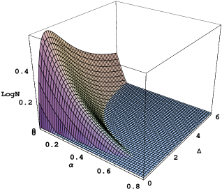
Figure 1: The stationary state log-negativity $N(\rho_{f})$ of the density operator $\rho_{f}(\infty)$ is plotted as a function of the mean photon number $\bar{m}_{1}=\bar{m}_{2}=\alpha$ of initial thermal fields and the detuning $\Delta$ with $g=0.5$ and $\theta=\frac{\pi}{2}$.

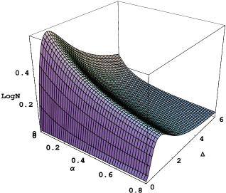
Figure 2: The stationary state log-negativity $N(\rho_{f})$ of the density operator $\rho_{f}(\infty)$ is plotted as a function of the mean photon number $\bar{m}_{2}=\alpha$ of second mode thermal field and the detuning $\Delta$ with $g=0.5$, $\bar{m}_{1}=0$ and $\theta=\frac{\pi}{2}$.

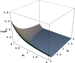
Figure 3: The stationary state log-negativity $N(\rho_{f})$ of the density operator $\rho_{f}(\infty)$ is plotted as a function of the mean photon number $\bar{m}_{1}$ and $\bar{m}_{2}$ of initial thermal fields with $g=0.5$, $\Delta=1$ and $\theta=\frac{\pi}{2}$.

In the resonant case, there is not any stationary state entanglement between the two modes. Nevertheless, the entanglement still arise in the forepart of the evolution, if either the initial temperature of the thermal fields or the phase decoherence coefficient are not too large. In Fig.4, the log-negativity $N(\rho_{f})$ of the time evolution density operator $\rho_{f}(t)$ is plotted as a function of the mean photon number $\bar{m}_{1}=\bar{m}_{2}=\alpha$ of initial thermal fields and the time $t$. It is shown that the two-mode fields can get entangled in the beginning of the time evolution, and become disentangled due to the presence of decoherence. However, in the off-resonant case, the entanglement is robust against the phase decoherence. Fig.5 clearly displays how the two initial thermal fields get entangled and eventually evolve into a stationary entangled state. When the two fields are initially in thermal states, the higher the temperature, the later the onset of entanglement between two fields. There will not be any entanglement appearing between two fields as their initial temperature exceeds certain threshold value which depends on the decoherence coefficient, the coupling strength and the detuning. Furthermore, we plot the log-negativity as the function of the time and the mean number difference $\delta=|\bar{m}_{1}-\bar{m}_{2}|$ with a fixed mean number sum $\bar{m}_{1}+\bar{m}_{2}=1$. It is shown that the log-negativity increases with the number difference at any time. In the case with $\omega_{1}=\omega_{2}$, increasing the difference of initial temperature of two thermal field results in enlarging the value of $\delta$. So, one can improve the entanglement by increasing the temperature difference in the situation that the total energy of the initial thermal fields is fixed. The novel phenomena that increasing the temperature difference of the thermal fields will improve their entanglement may have some applications in the quantum information processing, in which some subsystems are initially in thermal equilibrium.

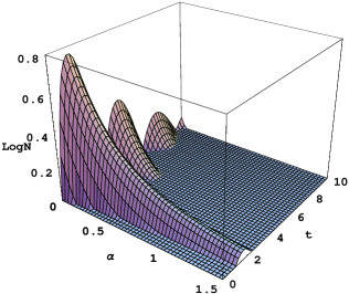
Figure 4: The log-negativity $N(\rho_{f})$ of the time evolution density operator $\rho_{f}(t)$ is plotted as a function of the mean photon number $\bar{m}_{1}=\bar{m}_{2}=\alpha$ of initial thermal fields and the time $t$ with $g=0.5$, $\theta=\frac{\pi}{2}$, $\gamma=0.5$ and $\Delta=0$.

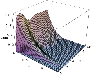
Figure 5: The log-negativity $N(\rho_{f})$ of the time evolution density operator $\rho_{f}(t)$ is plotted as a function of the mean photon number $\bar{m}_{1}=\bar{m}_{2}=\alpha$ of initial thermal fields and the time $t$ with $g=0.5$, $\theta=\frac{\pi}{2}$, $\gamma=0.5$ and $\Delta=1$.

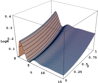
Figure 6: The log-negativity $N(\rho_{f})$ of the time evolution density operator $\rho_{f}(t)$ is plotted as a function of the mean photon number difference $\delta=|\bar{m}_{1}-\bar{m}_{2}|$ of initial thermal fields and the time $t$ with $g=0.5$, $\theta=\frac{\pi}{2}$, $\gamma=0.5$, $\bar{m}_{1}+\bar{m}_{2}=1$ and $\Delta=1$.

IV. CONCLUSION

In this paper, we investigate a possible scheme for entangling two mode thermal fields through the quantum erasing process, in which an atom is coupled with two mode fields via the interaction governed by the two-mode two-photon Jaynes-Cummings model. The influence of phase decoherence on the entanglement of two mode fields is discussed. It is found that quantum erasing process can transfer part of entanglement between the atom and fields to two mode fields initially in the thermal states. The entanglement achieved by fields heavily depends on their initial temperature and the detuning. The entanglement of stationary state is also investigated. It is interesting to study the entanglement in a similar scheme in which the two-mode two-photon Jaynes-Cummings model is replaced by the two-mode Raman coupling Jaynes-Cummings model. Both schemes can be easily realized in the two-dimensional ion trap. The details will be discussed elsewhere.

ACNOWLEDGMENT

This project was supported by the National Natural Science Foundation of China (Project NO. 10174066).

References

• [1] A. Einstein, B. Podolsky and N. Rosen, Phys. Rev. 47, 777(1935).
• [2] M.C. Arnesen, S. Bose, and V. Vedral, Phys. Rev. Lett. 87, 017901 (2001).
• [3] M.B. Plenio, S.F. Huelga, Phys. Rev. Lett. 88, 197901 (2002).
• [4] M.S. Kim, J. Lee, D. Ahn, P.L. Knight, Phys. Rev. A 65, 040101(R) (2002).
• [5] S.-B. Li, J.-B. Xu, Phys. Lett. A 313, 175 (2003).
• [6] M.O. Scully and K. Drüll, Phys. Rev. A 25, 2208 (1982).
• [7] M.H. Rubin, Phys. Rev. A 61, 022311 (2000).
• [8] Jing-Bo Xu and Xu-Bo Zou, Phys. Rev. A 60, 4743 (1999).
• [9] Jing-Bo Xu, Xu-Bo Zou and Ji-Hua Yu, Eur. Phys. J. D 10, 295 (2000).
• [10] S.-C. Gou, Phys. Rev. A 40, 5116 (1989).
• [11] C. W. Gardiner, Quantum Noise (Springer-Verlag, Berlin, 1991).
• [12] G.M. Milburn, Phys. Rev. A 44, 5401 (1991).
• [13] H. Moya-Cessa et al., Phys. Rev. A 48, 3900 (1993).
• [14] G. Vidal, R.F. Werner, Phys. Rev. A 65, 032314 (2002).
• [15] S. Bose, I. Fuentes-Guridi, P.L. Knight, V. Vedral, Phys. Rev. Lett. 87, 05401 (2001).