Matched detectors as definers of force

Abstract

Although quantum states nicely express interference effects, outcomes of experimental trials show no states directly; they indicate properties of probability distributions for outcomes. We prove categorically that probability distributions leave open a choice of quantum states and operators and particles, resolvable only by a move beyond logic, which, inspired or not, can be characterized as a guess.

By recognizing guesswork as inescapable in choosing quantum states and particles, we free up the use of particles as theoretical inventions by which to describe experiments with devices, and thereby replace the postulate of state reductions by a theorem. By using the freedom to invent probe particles in modeling light detection, we develop a quantum model of the balancing of a light-induced force, with application to models and detecting devices by which to better distinguish one source of weak light from another. Finally, we uncover a symmetry between entangled states and entangled detectors, a dramatic example of how the judgment about what light state is generated by a source depends on choosing how to model the detector of that light.

and

1 Introduction

Connecting the bench of experiment and the blackboard of theory offers physicists opportunities for creativity that we propose to make explicit. Traditional views underplay the physicist’s role in making these connections. Although physicists have wished for mathematics that would connect directly to experiments on the bench, the equations of quantum mechanics express quantum states and operators not directly visible in spectrometers or other devices. Here we look into quantum mechanics as mathematical language used to model behaviors of devices arranged on the laboratory bench. After separating models as mathematical objects from any assertion that a certain model describes a given experiment with devices, we ask: given a certain form of model, which models, if any, fit the behavior of some particular devices on the bench? In contrast to any hope for a seamless, unique blackboard description of devices on a laboratory bench, we argue, based on mathematical proofs presented in Sec. 3, that no matter what experimental trials are made, if a quantum model generates calculated probabilities that match given experimentally determined relative frequencies, there are other quantum models that match as well but that differ in their predictions for experiments not yet performed.

The proofs demonstrate what before could only be suspected: between the two pillars of calculation and measurement must stand a third pillar of choice making, involving personal creativity beyond logic, so there can be no reason to expect or demand that any two people choose alike.

What does recognizing choice mean for physicists? In physics, as in artistic work, pleasure and joy come from the choices one makes that lead to something interesting. Looking back, physicists can hardly help noticing that their proudest accomplishments, whether theoretical or experimental, have involved choices made by reaching beyond logic on the basis of intuition, hunches, analogies—some kind of guess, perhaps inspired, but still outside of logic. To understand the proofs is to see opportunities for making guesses. Although hunches and guesses and intuition can be as personal as dreams, the recognition of guesswork as a permanent pillar of physics has more than personal impact:

1. Describing device behavior will be recognized in Sec. 4 as a bi-lingual enterprise, with a language of wrenches and lenses for experimental trials on the bench and a different language of states and operators for the blackboard, linked by metaphors as guesswork. We show how freedom to choose particles as constituents of models of devices both helps in modeling devices and allows us to replace a widespread but questionable postulate of “state reductions” by a theorem.

2. The need for bi-lingual descriptions bridging bench and blackboard gives local color to certain concepts. In Sec. 5 we develop a notion of force in the context of light detection that gives meaning both at the blackboard and the bench not only to expectation values of light forces, but also to higher-order statistics associated with them, with application to models and detecting devices by which to better distinguish one source of weak light from another.

3. In Sec. 6 we uncover a symmetry, pertaining to entanglement, to make vivid the way judgments about how to model light are interdependent with judgments about how to model light-detectors.

2 Models mathematically distinct from experiments

Experimental records can hold: (1) numerals interpreted as the settings of knobs that control an experiment, and (2) numerals interpreted as experimental outcomes, thought of as the clicks and flashes and electronically tallied pulses by which the devices used in the laboratory respond to and measure whatever is at issue. As an abstraction by which one can model experimental outcomes, quantum theory offers what we shall call theoretical outcomes (referred to in the literature variously as outcomes, results, the finding of particles and the finding of states). Probabilities of theoretical outcomes are expressed in terms of states and operators by what we shall call quantum models. We discuss these first, and then distinguish the probabilities expressed by models from relative frequencies of experimental outcomes.

2.1 Definition of quantum-mechanical models

The propositions about linking models to devices (Sec. 3) can be proved using any formulation of quantum mechanics that includes probabilities of theoretical outcomes. Here is a standard formulation taken from Dirac [1] and von Neumann [2], bulwarked by a little measure theory [3]; however, as discussed in Sec. 4, we invoke no postulate of state reductions.

Let $H$ be a Hilbert space, let $\rho$ be any self-adjoint operator of unit trace on $H$ (otherwise known as a density operator), and let $M$ be a $\sigma$-algebra of subsets of a set $\Omega$ of possible theoretical outcomes. By a theoretical outcome we mean a number or a list of numbers as a mathematical object, in contrast to an experimental outcome extracted from an experimental record. Let $E$ be any projective resolution on $M$ of the identity operator on $H$ (which implies that for any $\omega\in M$, $E(\omega)$ is a self-adjoint projection [4]). Let $U(t)$ be a unitary time-evolution operator (typically defined by a Schrödinger equation or one of its relativistic generalizations). These mathematical objects can be combined to define a probability distribution $\mu$ on $M$, parameterized by $t$:

$$\mu(t)(\omega)\stackrel{{\scriptstyle\rm def}}{{=}}\mathrm{Tr}[U(t)\rho U^{\dagger}(t)E(\omega)],$$ (1)

where $\mu(t)(\omega)$ is the probability of an outcome in the subset $\omega$ of $\Omega$, for the parameter value $t$.

For a probability $\mu(t)(\omega)$ to be compared to anything experimental, one needs to make explicit the dependence of the $\rho$ and $E$ that generate it on the experimentally controllable parameters. It is convenient to think of these parameters as the settings of various knobs; to express them we let $A$ and $B$ be mathematically arbitrary sets (interpreted as sets of knob settings). Let $\mathcal{D}$ be the set of functions from $A$ to density operators acting on $H$. Let $\mathcal{E}$ be the set of functions from $B$ to projective resolutions of the identity on $M$ of the identity operator on $H$. Then what we shall call a specific quantum model is a triple of functions $(\rho,E,U)$ together with $\rho\in\mathcal{D}$, $E\in\mathcal{E}$, and $U(t)$ a unitary evolution operator. By the basic rule of quantum mechanics, such a specific quantum model generates a probability-distribution as a function of knob settings and time:

$$(\forall\ a\in A,\ b\in B,\ t\in I,\ \omega\in M)$$

$$\qquad\mu(a,b,t)(\omega)=\mathrm{Tr}[U(t)\rho(a)U^{\dagger}(t)E(b)(\omega)].$$ (2)

Often one needs something less specific than a triple $(\rho,E,U)$. By a model we shall mean a set of properties of that limit but need not fully specify $\rho$, $U$, and $E$. For example, in modeling entangled light, we might construct a model in this sense by specifying relevant symmetry properties of $E$, $U$, and $\rho$, leaving many fine points unspecified.

Remarks

1. An element $a\in A$ can be a list: $a=\{a^{(1)},\dots,a^{(n)}\}$; similarly an element $b\in B$ can be a list.

2. By the domain of a model, we mean the cartesian product of the sets $A\times B\times I\times M$. Models of a given domain can differ as to the functions $\rho$, $E$, and $U$ defined on the sets $A$, $B\times M$, and $I$, respectively, so that different models with a given domain can differ in the states, operators, and probabilities that they assert.

3. In defining the domain of a model, we view $\mu$ as a function from $A\times B\times I\times M\rightarrow[0,1]$, but in writing the left side of Eq. (2) we take the alternative view of $\mu$ as a function $A\times B\times I\rightarrow\{\mbox{probability measures on }M\}$.

4. Different specific models can be distinguished by labels: a model $\alpha$ consisting of $(\rho_{\alpha},U_{\alpha},E_{\alpha})$ generates a probability function $\mu_{\alpha}$. Because $\mu_{\alpha}$ is invariant under any unitary transformation applied to all three of $\rho_{\alpha}$, $E_{\alpha}$, and $U_{\alpha}$, an important feature of the states asserted by a specific model $\alpha$ is the unitary-invariant overlap between pairs of them. The measure of overlap convenient to Sec. 3 is

   $$\mathrm{Overlap}(\rho_{\alpha}(a_{1}),\rho_{\alpha}(a_{2}))\mathop{\stackrel{{\scriptstyle\mathrm{def}}}{{=}}}\nolimits\mathrm{Tr}[\rho_{\alpha}(a_{1})^{1/2}\rho_{\alpha}(a_{2})^{1/2}].$$ (3)

   We express the difference in state preparations asserted by specific models $\alpha$ and $\beta$ having the same domain for elements $a_{1},a_{2}\in A_{\alpha}\cap A_{\beta}$ by $|\mathrm{Overlap}(\rho_{\alpha}(a_{1}),\rho_{\alpha}(a_{2}))-\mathrm{Overlap}(\rho_{\beta}(a_{1}),\rho_{\beta}(a_{2}))|$.

5. We call a model $\beta$ a restriction of a model $\alpha$ if the domain of model $\beta$ is a subset of the domain of model $\alpha$.

2.2 Domains of models and of experimental records

So much for quantum models as mathematical objects; how do we compare probabilities from these models with results of an experiment with lasers and lenses and other devices? First one contrives to view the experiment as consisting of trials, each for certain settings of some knobs, yielding at each trial one of several possible experimental outcomes. By tallying the experimental outcomes for various knob settings, one extracts from the experimental record the relative frequencies of experimental outcomes as a function on a domain of experimental knob settings and outcomes.

To compare experimental relative frequencies with probabilities calculated from a model, both viewed as functions on domains of knob settings and outcome bins, it is necessary to identify the experimental domain as a subset of the model domain. This entails associating to each experimental outcome $c$ some model outcome $\omega_{c}\in M$. For the experimental relative-frequency of outcome $c$ for each setting of knobs $(a,b,t)$ in the experimentally covered subset of $A\times B\times I$ we write $\nu_{r}(a,b,t)(c)$; this is the ratio of the number of trials with knob settings and time $(a,b,t)$ and an experimental outcome in $c$ to the number of trials with knob settings and time $(a,b,t)$ regardless of the outcome. Letting $C$ denote the set of experimental outcomes, one has

$$(\forall\ t\in I,\ a\in A,\ b\in B)\quad\sum_{c\in C}\nu_{r}(a,b,t)(c)=1.$$ (4)

By virtue of the mapping $c\mapsto\omega_{c}\subset\Omega$, one can compare the experimental relative-frequency function $\nu_{r}$ with the probability function $\mu_{\alpha}$ asserted by any model $\alpha$ having a domain containing a subset identified with the domain of the experimental relative frequencies. Because of this need for identification, a choice of model domain constrains the design, or at least the interpretation, of experimental records to which models of that domain can be compared. In compensation, committing oneself to thinking about an experimental endeavor in terms of a particular model domain makes it possible to:

1. organize experiments to generate data that can be compared with models having that domain;

2. express the results of an experiment mathematically without having to assert that the results fit any particular model;

3. pose the question of whether the experimental data fit one model having that domain better than they fit another model [5].

3 Choosing a model to fit given probabilities

What can relative frequencies of outcomes of experimental trials of devices tell us about how to model those devices? At best, from relative frequencies of experimental outcomes as a function of knob settings, as in Eq. (4), one abstracts an approximation to a probability-distribution function of knob settings. By ignoring statistical and other error, we picture an ideal case of arriving at some $\mu_{\alpha}(a,b)(\omega)$, but without any further information concerning the states or operators that generate it. This raises a question inverse to the text-book task of calculating probabilities from states and operators: given the probability function $\mu_{\alpha}(a,b)(\omega)$, what states and operators generate it via the rule of Eq. (2)? Put another way, what are the constraints and freedoms on a density-operator function $\rho$, an evolution operator $U(t)$, and a measurement-function $E$ if these are to generate a given probability function $\mu_{\alpha}(a,b)(\omega)$ via the rule of Eq. (2)? Here are some answers.

3.1 Constraint on density operators

If for some values $a_{1}$, $a_{2}$, $b$, and $\omega$ one has $\mu(a_{1},b,t)(\omega)$ large and $\mu(a_{2},b,t)(\omega)$ small, then Eq. (2) implies that $\rho(a_{1})$ is significantly different from $\rho(a_{2})$. This can be quantified in terms of the overlap of two density operators $\rho(a_{1})$ and $\rho(a_{2})$ defined in Eq. (3).

Proposition 1:  For a specific model $(\rho,E,U)$ to be consistent with a probability function $\mu$ in the sense of Eq. (2), the overlap of density operators for distinct knob settings $a_{1}$ and $a_{2}$ has an upper bound given by

$$(\forall\ a_{1},a_{2}\in A)$$

$$\mathrm{Tr}[\rho(a_{1})^{1/2}\rho(a_{2})^{1/2}]\leq\min_{b,t,\omega}\{[\mu(a_{2},b,t)(\omega)]^{1/2}+[1-\mu(a_{1},b,t)(\omega)]^{1/2}\}.$$

Proof:  For purposes of the proof, abbreviate $\rho(a_{1})$ by $a_{1}$, $\rho(a_{2})$ by $a_{2}$, and $U^{\dagger}(t)E(b)U(t)(\omega)$ by $E$. Because $E$ is a projection, $E=E^{2}$. Then the Schwarz inequality and a little algebra implies

$$|\mathrm{Tr}(a_{1}^{1/2}a_{2}^{1/2})| = |\mathrm{Tr}(a_{1}^{1/2}Ea_{2}^{1/2})+\mathrm{Tr}(a_{1}^{1/2}(1-E)a_{2}^{1/2})|$$ (6)

$$\leq |\mathrm{Tr}(a_{1}^{1/2}Ea_{2}^{1/2})|+|\mathrm{Tr}(a_{1}^{1/2}(1-E)a_{2}^{1/2})|$$

$$\leq (\mathrm{Tr}\,a_{1})^{1/2}[\mathrm{Tr}(Ea_{2}^{1/2}a_{2}^{1/2}E)]^{1/2}$$

$$\mbox{}+[\mathrm{Tr}(a_{1}^{1/2}(1-E)(1-E)a_{1}^{1/2})]^{1/2}(\mathrm{Tr}\,a_{2})^{1/2}$$

$$= [\mathrm{Tr}(Ea_{2}^{1/2}a_{2}^{1/2}E)]^{1/2}+[\mathrm{Tr}(a_{1}^{1/2}(1-E)(1-E)a_{1}^{1/2})]^{1/2}$$

$$= [\mathrm{Tr}(a_{2}E)]^{1/2}+[1-\mathrm{Tr}(a_{1}E)]^{1/2}.$$

Expanding the notation, we have

$$(\forall\ a_{1},a_{2}\in A)$$

$$\qquad\mathrm{Tr}[\rho(a_{1})^{1/2}\rho(a_{2})^{1/2}]\leq\min_{b,t,\omega}\{[\mathrm{Tr}(\rho(a_{2})U^{\dagger}(t)E(b)(\omega)U(t))]^{1/2}$$

$$\hskip 133.69994pt\mbox{}+[1-\mathrm{Tr}(\rho(a_{1})U^{\dagger}(t)E(b)(\omega)U(t))]^{1/2}\},$$ (7)

which, with Eq. (2), completes the proof. $\Box$

Example:  For $0\leq\epsilon,\delta\ll 1$, if for some $b$ and $\omega$, $\mu(a_{2},b,t)(\omega)=\epsilon$ and $\mu(a_{1},b,t)(\omega)$ $=1-\delta$, then it follows that $\mathrm{Tr}[\rho(a_{1})^{1/2}\rho(a_{2})^{1/2}]\leq\epsilon^{1/2}+\delta^{1/2}$. If, in addition, $\rho(a_{1})=|a_{1}\rangle\langle a_{1}|$ and $\rho(a_{2})=|a_{2}\rangle\langle a_{2}|$, then we have $|\langle a_{1}|a_{2}\rangle|^{2}\leq\epsilon^{1/2}+\delta^{1/2}$.

3.2 Freedom of choice for density operators

The preceding proof of an upper bound invites the question: is there a corresponding positive lower bound? The answer turns out to be “no.”

Proposition 2:  For any specific model $(\rho_{\alpha},E_{\alpha},U_{\alpha})$ and any knob settings $a_{1},a_{2}\in A$, regardless of Overlap$(\rho_{\alpha}(a_{1}),\rho_{\alpha}(a_{2}))$ there is a specific model $(\rho_{\beta},E_{\beta},U_{\beta})$ with $\mu_{\beta}=\mu_{\alpha}$ and Overlap$(\rho_{\beta}(a_{1}),\rho_{\beta}(a_{2}))=0$.

Proof by construction:  Let $H_{\beta}$ be the direct sum of three Hilbert spaces $H_{0}$, $H_{1}$, and $H_{2}$, each a copy of the Hilbert space $H_{\alpha}$ of model $\alpha$: $H_{\beta}=H_{0}\oplus H_{1}\oplus H_{2}$. Let $E_{\beta}(b)(c)$ be the direct sum of three copies of $E_{\alpha}(b)(c)$, one for each of the $H_{j}$; similarly, let $U_{\beta}$ be the direct sum of three copies of $U_{\alpha}$. Define $\rho_{\beta}$ by

$$\rho_{\beta}(a)=\begin{cases}\ \rho_{\alpha}\oplus 0\oplus 0&\mbox{\ if \ }a\neq a_{1}\mbox{\ and\ }a\neq a_{2};\\ \ 0\oplus\rho(a_{1})\oplus 0&\mbox{\ if \ }a=a_{1};\\ \ 0\oplus 0\oplus\rho(a_{2})&\mbox{\ if \ }a=a_{2}.\end{cases}$$ (8)

This defines a model $\beta$ of the form of Eq. (2) for which we have

$$(\forall\ a\in A,\ b\in B,\ t\in I,\ \omega\in M)\hskip 10.00002pt\mu_{\alpha}(a,b,t)(\omega)=\mu_{\beta}(a,b,t)(\omega),$$ (9)

but for the Overlap as defined in Eq. (3), $\mathrm{Overlap}(\rho_{\beta}(a_{1}),\rho_{\beta}(a_{2}))=0$, regardless of the value of $\mathrm{Overlap}(\rho_{\alpha}(a_{1}),\rho_{\alpha}(a_{2}))$. $\Box$

This proof shows the impossibility of establishing by experiment a positive lower bound on state overlap without reaching outside of logic to make an assumption, or, to put it baldly, to guess [5]. The need for a guess, no matter how educated, has the following interesting implication. Any experimental demonstration of quantum superposition depends on showing that two different settings of the $A$-knob produce states that have a positive overlap. For example, a superposition $|a_{3}\rangle=(|a_{1}\rangle+e^{i\phi}|a_{2}\rangle)/\sqrt{2}$ has a positive overlap with state $|a_{1}\rangle$. Because, by Proposition 2, no positive overlap is experimentally demonstrable without guesswork, we have the following:

Corollary to Proposition 2:  Experimental demonstration of the superposition of states requires resort to guesswork.

3.3 Constraint on resolutions of the identity

Much the same story of constraint and freedom holds for resolutions of the identity. For the norm of an operator $A$ we take $\|A\|=\sup_{u}\|Au\|$, where $u$ ranges over all unit vectors. Then we have:

Proposition 3:  In order for a specific model $(\rho,E,U)$ to generate a given probability function $\mu$, the resolution of the identity must satisfy the constraint

$$\|E(b_{1})(\omega_{c})-E(b_{2})(\omega_{c})\|\geq\max_{a\in A,\,t\in I}|\mu(a,b_{1},t)(c)-\mu(a,b_{2},t)(c)|.$$

Proof:  Replacing unit vectors by density operators in the definition of the norm results in the same norm, from which we have

$$\|E(b_{1})(\omega_{c})-E(b_{2})(\omega_{c})\| \geq \max_{a\in A,\,t\in I}|\mathrm{Tr}[U(t)\rho(a)U^{\dagger}(t)E(b_{1})(\omega_{c})]$$

$$\mbox{}-\mathrm{Tr}[\rho(a)E(b_{2})(\omega_{c})]|$$

$$= \max_{a\in A,\,t\in I}|\mu(a,b_{1})(c)-\mu(a,b_{2})(c)|.$$

$$\hskip 209.58255pt\Box$$

3.4 Freedom of choice for resolutions of the identity

The difference of any two commuting projections has norm less than or equal to 1. Can requiring a model $\alpha$ to generate a given probability function $\mu$ impose any upper bound less than 1 on $\|E_{\alpha}(b_{1})(\omega_{c})-E_{\alpha}(b_{2})(\omega_{c})\|$?

Proposition 4: For any specific model $(\rho_{\alpha},E_{\alpha},U_{\alpha})$ and any knob settings $b_{1}$ and $b_{2}$, regardless of $\|E_{\alpha}(b_{1})(\omega_{c})-E_{\alpha}(b_{2})(\omega_{c})\|$ there is a specific model $(\rho_{\beta},E_{\beta},U_{\beta})$ with $\mu_{\beta}=\mu_{\alpha}$ and $\|E_{\beta}(b_{1})(\omega_{c})-E_{\beta}(b_{2})(\omega_{c})\|=1$.

Proof by construction:  Let the Hilbert space for model $\beta$ be $H_{\beta}=H_{\alpha}\oplus H_{\perp}$ where $H_{\perp}$ is a space orthogonal to $H_{\alpha}$. Let $E_{\beta}(b_{1})(\omega_{c})=E_{\alpha}(b_{1})(\omega_{c})\oplus\mathbf{1}_{\perp}$ and $E_{\beta}(b_{2})(\omega_{c})=E_{\alpha}(b_{2})(\omega_{c})\oplus\mathbf{0}_{\perp}$, where $\mathbf{1}_{\perp}$ is the unit operator on $H_{\perp}$ and $\mathbf{0}_{\perp}$ is the zero operator on $H_{\perp}$. Let $\rho_{\beta}=\rho_{\alpha}\oplus\mathbf{0}_{\perp}$. Then, $\|E_{\alpha}(b_{1})(\omega_{c})-E_{\alpha}(b_{2})(\omega_{c})\|$$=1$. $\Box$

Remark: Suppose, as displayed in the proof of Proposition 2, models $\alpha$ and $\beta$ have the same domain and $\mu_{\alpha}$ = $\mu_{\beta}$, but the $\alpha$-states have overlaps differing from those of the $\beta$-states. Then there is always a resolution of the identity $E^{\prime}$ outside the range of $E_{\alpha}$ and $E_{\beta}$, such that for some $a$, $\,\mbox{Tr}[\rho_{\alpha}(a)E^{\prime}]\neq\mbox{Tr}[\rho_{\alpha}(a)E^{\prime}]$. In this sense the models $\alpha$ and $\beta$ conflict concerning their predictions [6].

4 Impact on quantum physics

The connection of any specific quantum model to experiments is via a probability function. This and the proofs of Propositions 2 and 4 show something that experiments cannot show, namely that modeling an experiment takes guesswork, and that a model, once guessed, is subject to surprises arising in experiments not yet performed. Some guesses get tested (one speaks of hypotheses), but testing a guess requires other guesses not tested. By way of example, to guide the choice of a density operator by which to model the light emitted by a laser, one sets up the laser, filters, and a detector on a bench to produce experimental outcomes. But to arrive at any but the coarsest properties of a density operator one needs, in addition to these outcomes, a model of the detector, and concerning this model, there must always be room for doubt; we can try to characterize the detector better, but for that we have to assume a model for one or more sources of light. When we link bench and blackboard, we work in the high branches of a tree of assumptions, holding on by metaphors, where we can let go of one assumption only by taking hold of others. Because of the guesswork needed to bridge between models and experiments, describing device behavior is forever a bi-lingual enterprise, with a language of wrenches and lenses for the bench and a different language of states and operators for the blackboard.

We will show how some words work as metaphors, straddling bench and blackboard, where by ‘words’ we mean to include whatever mathematical symbols are used to describe devices. We consider the mathematics of quantum mechanics not in contrast to words but as blackboard language, words of which are sometimes borrowed for use at the bench to describe devices. By showing some choices of metaphorical uses of the words state, operator, spacetime, outcome, and particle, we promote freedom to invent particles as needed to describe interesting features of device behavior. Recognizing choices in word use reflects back on how we formulate quantum mechanics: the notion of repeated measurements ‘of a state’ will be revealed as neither necessary nor sensible, and the so-called postulate of state reductions will evaporate, leaving in its place a theorem.

4.1 Word use at blackboard and lab bench

We start by looking at several related but distinct uses of spacetime coordinates. In the laboratory one uses clocks and rulers to assign coordinates to acts of setting knobs, transmitting signals, recording detections, etc, and one thinks of these experimentally generated coordinates as points of a spacetime—something mathematical. We call this a ‘linear spacetime’ to distinguish it from a second spacetime, that we call ‘cyclic,’ onto which the linear spacetime is folded, like a thread wound around a circle, so that experimental outcomes for different trials can be tallied in bins labeled by coordinates. Distinct from linear and cyclic spacetimes, any quantum-mechanical model involves a third spacetime on which are defined solutions of a Schrödinger equation (or one of its relativistic generalizations), and it is with reference to this spacetime that particles as theoretical constructs are defined.

Any quantum model written in terms of particles generates probabilities, and if the probabilities of the model fit the relative frequencies of experimental outcomes well enough, one is tempted to say that one has “seen the particles”; however, because particles in their mathematical sense are creatures of models, and multiple, conflicting models are consistent with any given experimental data, this “seeing of particles” stands on guesswork and metaphor, needed, for example, to bind the electron as a solution of the Dirac equation defined on a model spacetime to a flash from a phosphor on a screen. This metaphorical role of electron, photon, etc., though habitual and easily overlooked, can be noticed when a surprise prompts one to make a change in the use of the word electron at the blackboard while leaving the use at the bench untouched, or vice versa.

Next we address notions of (a) components of a theoretical outcome, (b) a distinction between signal particles and probe particles, and (c) various measurement times. We take these in order.

4.1.1 Multiple components of an outcome

The term theoretical outcome pertains to a vector space of multi-particle wave functions defined on a model spacetime. This vector space is a tensor product of factors, one factor for each particle. For a resolution of the identity that factors accordingly, we shall view each theoretical outcome for this resolution as consisting of a list of components, one component for each of the factors. A probability density for such multi-component outcomes can be viewed as a joint probability density for the component parts of the outcome, modeling the joint statistics of the detection of many particles.

4.1.2 Signal and probe particles

We who model are always free to shift the boundary between states (as modeled by density operators) and measuring devices (as modeled by resolutions of the identity) so as to include more of the measuring devices within the scope of the density-operator part of the model [2]. Consider for example a coarse model $\alpha$ that portrays a detecting device by a resolution of the identity. While a resolution of the identity has no innards, detecting devices do. To model, say, a photo-diode and its accompanying circuitry, we can replace model $\alpha$ by a more detailed model $\beta$: the quantum state asserted by model $\alpha$ becomes what we call a signal state, a factor in a tensor product (or more generally a sum of tensor products) accompanied by factors for one or more probe-particle states. According to this model $\beta$, the signal state is measured only indirectly, via a probe state with which it has interacted, followed by a measurement of the probe states, as modeled by “a resolution of the identity” that works on the probe factor, not the signal factor.

4.1.3 Measurement times

Recognizing probe-states as free choices in modeling clarifies a variety of times relevant to quantum measurements. For any quantum model $\alpha$, the form of Eq. (2) links an outcome (whether single- or multi-component) to some point time $t_{\alpha}$; however, the use of such a model is to describe an actual or anticipated experiment, and for this, as described above, one is always free to choose a more detailed model $\beta$, in which the state of model $\alpha$ appears as the signal state that interacts with a probe state, followed by a measurement of the probe state at some time $t_{\beta}$ after the interaction. Thus model $\beta$ replaces the point time $t_{\alpha}$ by a time stretch during which the signal and probe states interact, thus separating the time during which the signal state interacts with the probe from the time at which the probe state is measured.

In more complex models involving more probe states, a succession of “times of measurement” in the sense of interactions can be expressed by a single resolution of the identity. Finally, in modeling spatially dispersed signal states that interact with entangled probe particles [7], one can notice a prior “probe-interaction time” during which the probe particles must interact with one another, in order to have become entangled.

4.2 State reduction as a theorem, not a postulate

Recognizing choice in modeling allows one to sidestep a long-troubling issue in formulating quantum language. In logical conflict with the Schrödinger equation as the means of describing time evolution [8], Dirac and other authors introduce state reductions by a special postulate that asserts an effect on a quantum state of a resolution of the identity; allegedly needed to express repeated measurements of a system. Once we recognize the modeling freedom to make signal-probe interactions explicit, we can always replace any story about devices involving a “state to be measured repeatedly” by a model in which a signal state interacts with a succession of probe states, followed by a simultaneous measurement of all the probe states, as expressed by a single resolution of the identity and a composite state that incorporates both signal and probe states. Thus any apparent need for a postulate to do with “repeated measurements” evaporates, and with it the unfortunate appearance of state reductions in a postulate.

Although inconsistent as a postulate, state reduction still works in many cases as a trick of calculation, as justified by the following theorem.

Theorem: Assume any specific model of the form Eq. (2), and assume $\omega=(j,k)$ is an outcome with components $j$ and $k$. If $E(b)(j,k)$ is a tensor product $E(b)(j,k)=E_{A}(b)(j)\otimes E_{B}(b)$, then for any density-operator function $\rho(a)$, the joint probability distribution $\mu(a,b)(j,k)$ induces a conditional probability distribution for $k$ given $j$ that matches the quantum probability of $k$ obtained using a “reduced density operator” obtained by the usual rule for state reduction applied to $\rho$.

Proof: Streamline notation by suppressing the dependence on $a$ and $b$, and incorporate $U$ into $\rho$, so that the relevant form is that of Eq. (1). For any state $\rho$ it follows from Eq. (1) that $\Pr(j,k)=\mbox{Tr}[\rho(E_{A}(j)\otimes E_{B}(k))]$. The conditional probability of $k$ given $j$ is defined by Bayes rule [9]:

$$\Pr(k|j) = \frac{\Pr(j,k)}{\Pr(j)}=\frac{\Pr(j,k)}{\sum_{k^{\prime}}\Pr(j,k^{\prime})}=\frac{\mbox{Tr}[\rho(E_{A}(j)\otimes E_{B}(k))]}{\mbox{Tr}[\rho(E_{A}(j)\otimes\sum_{k^{\prime}}E_{B}(k^{\prime}))]}.$$ (10)

By the definition of a resolution of the identity, we have $\sum_{k^{\prime}}E_{B}(k^{\prime})=1$; recalling that $E_{B}(k)$ is a projection that commutes with $E_{A}(j)$, one then has

$$\Pr(k|j)=\mbox{Tr}[\rho_{\rm red}E_{B}(k)],$$ (11)

for an operator

$$\rho_{\rm red}\stackrel{{\scriptstyle\rm def}}{{=}}\frac{E_{A}(j)\rho E_{A}(j)}{\mbox{Tr}[E_{A}(j)\rho E_{A}(j)]}.$$ (12)

This $\rho_{\rm red}$ matches the ‘reduced density operator’ obtained by the usual rule of state reduction. Q.E.D.

Remarks:

1. In case $\rho=|\psi\rangle\langle\psi|$ is a pure state, then $\rho_{\rm red}=|\psi_{\rm red}\rangle\langle\psi_{\rm red}|$, where the reduced state

   $$|\psi_{\rm red}\rangle=\frac{E_{A}(j)|\psi\rangle}{\|E_{A}(j)|\psi\rangle\|},$$ (13)

   which is one form of the usual rule for state reduction, but here obtained by calculation with no need for any postulate.

2. Either of the outcome components can be a composite, so the theorem applies to cases involving more than two outcome components.

3. In relativistic formulations of quantum mechanics, detections at spatially separated locations $A$ and $B$ can be modeled by projections of the form assumed.

5 Balancing forces in the detection of weak light

Of interest in particle physics, astrophysics, and emerging practical applications, sources of weak light are characterized experimentally by the experimental outcomes of detectors [10]. Because detector outcomes are statistical, trial-to-trial differences in outcomes can arise both from trial-to-trial irregularity in the sources and from quantum indeterminacy in their detection. As we shall see, detecting devices work in two parts, one of which balances a light-induced force against some reference. By taking advantage of the freedom to invent probe particles when we model particle detectors, we are led to a quantum mechanical expression of force in the context of balancing devices, with application to models and detecting devices by which to better distinguish one source of weak light from another.

In Newtonian physics, the word force is used both on the blackboard and with balancing devices. In quantum physics, force, as used at the blackboard, gets re-defined in terms of the expectation values pertaining to dynamics of wave functions [11]. We will find useful a concept of force in characterizing light. Because of its employment in experimental work, our concept of force necessarily takes on local coloring special to one or another experimental bench; we develop a notion of force in the context of light detection that gives meaning both at the blackboard and the bench not only to expectation values of forces, but also to higher-order statistics associated with them. These higher-order statistics allow the expression, within quantum mechanics, of the teetering of a balance that happens when forces are nearly equal. We begin by reviewing some details of detector behavior.

5.1 Balancing in detectors

Under circumstances to be explored, particle detectors employed to decide among possible quantum states produce unambiguous experimental outcomes. Seen up close, a detecting device consists of two components. The first is a transducer such as a photo-diode that responds to light by generating a small current pulse. To tally a transducer response as corresponding to one or another theoretical outcome in the sense of quantum mechanics, one has to classify the response using some chosen criterion. As phrased in the engineering language of inputs and outputs, the response of the transducer is fed as an input to a second component of the detector, in effect an unstable balance implemented as a flip flop (made of transistors organized into a cross-coupled differential amplifier). The flip-flop produces an output intended to announce a decision between two possible experimental outcomes, say 0 and 1.

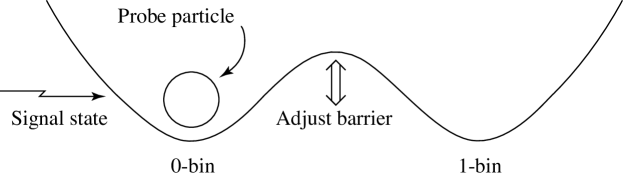
Figure 1: Detector as probe particle in a double well.

If we think classically, we picture the flip-flop as a ball and two bins, one bin for each possible outcome, separated by a barrier, the height of which can be adjusted, as shown in Fig. 1. The ball, starting in bin 0 is kicked by the transducer; an outcome of 1 is recorded if and only if the balance is tipped and the ball rolls past the barrier into bin 1. This ball-and-bin technique avoids ambiguity by virtue of a convention that gives the record a certain leeway: it does not matter if the ball is a little off center in its bin, so long as the ball does not teeter on the barrier between bins.

Although usually producing an unambiguous outcome, the flip-flop, seen up close, can teeter in its balancing, perhaps for a long time, before slipping into one bin or the other [12, 13]. Absent some special intervention, two parties (people or machines) to which a teetering output fans out can differ in how they classify this output as an outcome: one finds a 0, the other finds a 1. To reduce the risk of disagreement, the two parties have to delay their reading of the output, hopefully until the ball slips into one or the other bin.

Ugly in this classical cartoon are two related features: (1) the ball can teeter forever, so that waiting is no help, and (2) the mean time for teetering to end is entirely dependent on some ad hoc assumption about “noise” [12, 13]. Although we have described the flip-flop classically, it is built of silicon and glass presumably amenable to quantum modeling. To see what quantum models offer us, the first step is to recall that a quantum model implies probabilities to be related to an experiment, so that inventing a quantum model and choosing an experimental design go hand in hand. Thirty years ago, thinking not in quantum but in circuit terms, we designed and carried out an experiment to measure teetering of the output of a flip-flop. As we recognized only recently, the record of this experiment is compatible with some quantum models. A quantum model to be offered shortly describes the experiment already performed and serves as a guide for designing future experiments to exploit what can be called a statistical texture of force, previously obscured by the “noise” invoked in classical analysis.

5.2 Experimental design

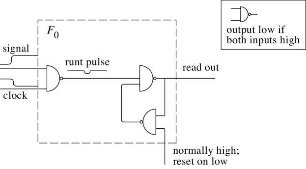
Figure 2: Flip-flop exposed to race between signal going high and clock going low.

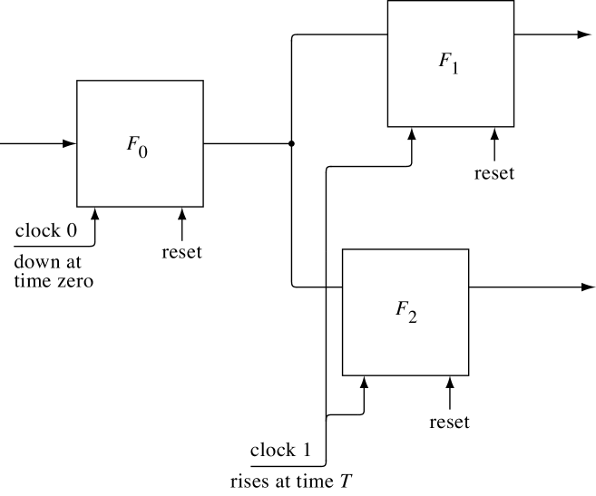
Figure 3: Flip-flops $F_{1}$ and $F_{2}$ used to read $F_{0}$ after a delay $T$.

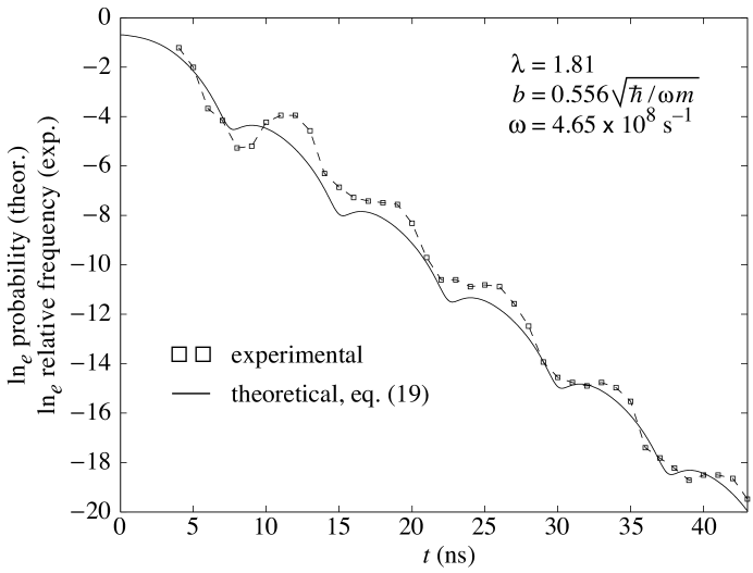
Figure 4: Probability of disagreement vs. settling time.

To experiment with the teetering of a detecting device comprised of a transducer $D_{0}$ (for diode) connected to a flip-flop $F_{0}$, shown in Fig. 2, we replace the transducer $D_{0}$ by a laboratory generator of weak electrical pulses to drive $F_{0}$. Putting the flip-flop $F_{0}$ into a teetering state takes very sensitive adjustment of the pulse generator, achieved by feedback from a running average of the outcomes produced by $F_{1}$ and $F_{2}$ to the pulse generator. The output of $F_{0}$ is made to fan out, as shown in Fig. 3, to a matched pair of flip-flops, $F_{1}$ and $F_{2}$, each of which acts as an auxiliary detector, not of the incoming light but of the output of $F_{0}$. The flip-flops $F_{1}$ and $F_{2}$ are clocked at a time $T$ later than is $F_{0}$. The experimental outcome consists of two binary components, one from $F_{1}$ and the other from $F_{2}$. If after the waiting time $T$ the output of $F_{0}$ is still teetering, the flip-flops $F_{1}$ and $F_{2}$ can differ, one registering a 1 while the other registers a 0; the disagreement between the two flip-flops registers the teetering of the output of $F_{0}$. The measured relative frequency of disagreements between $F_{1}$ and $F_{2}$ is shown in Fig. 4.

5.3 Quantum modeling of balancing in detectors

We want to model the teetering statistics that we will use to discriminate among various sources of weak signals. Traditional analyses of solid-state detecting devices and their flip-flops invoke quantum mechanics only to determine parameters for classical stories involving voltage and current. Analyzed that way, teetering in a photo-diode-based detector that employs a flip-flop made of transistors arises in two ways: first, there can be teetering in the entry of electrons and holes into the conduction band of the photo-diode; second, there can be teetering in the response of $F_{0}$ to whatever amplified pulse comes from the photo-diode. Although both these teeterings involve electrons and holes going into a conduction band, the statistical spread of outputs for a given state is blamed on noise unconnected with the signal, and known analyses of a flip-flop invoke noise to evade the embarrassment of a possible infinite hesitation.

Avoiding the invocation of ‘noise,’ we picture $F_{0}$ quantum mechanically as a pair of probe particles. Light acting via the transducer applies a force to the two probe particles. This scattering process transforms an initially prepared state of the light and probes to an out-state consisting of a sum (or integral) of products, each of which has a factor for the light and a factor for the two probe particles of $F_{0}$. After some waiting time of evolution $T$, the two probe particles are measured, as expressed by a resolution of the identity that ignores the signal state; thus the probabilities of theoretical outcomes of the detection after the interaction are expressible by a reduced density operator obtained by tracing over the signal states. In this view, teetering shows up in the probability of detecting the two probe particles on different sides of a reference; we will show how this probability depends on both the signal detected and a waiting time $T$, and how in this dependence Planck’s constant enters.

In the model presented here, we simplify the effect of the signal state to that of preparing, at time 0, a pair of probe-particle wave functions. For simplicity, the probe-particle wave functions have only one space dimension. Let $x$ be the space coordinate for one probe particle and $y$ be the space coordinate for the other. The difference between one possible signal state and another is reflected by concentrating the initial probe-state wave functions slightly to one side or the other of an energy hump centered at the origin $x=0$, $y=0$. (As might be expected, teetering is most pronounced in the borderline case of a signal state that puts the initial probe-particle wave functions evenly over the energy hump.) We model the flip-flop $F_{1}$ as a resolution of the identity that has an theoretical outcome of 1 for $x>0$ and 0 for $x<0$; similarly $F_{2}$ is modeled as a resolution of the identity for $y$. Thus the two-component theoretical outcomes are 00 for $x,y<0$; 01 for $x<0$, $y>0$; 10 for $x>0$, $y<0$; and 11 for $x,y>0$. By assuming a coupling between the two probe particles, we will model how increasing the waiting until time $T$ to detect the probe particles decreases the probability of disagreement between $F_{1}$ and $F_{2}$, i.e. diminishes the probability of $x$ and $y$ being measured with different signs.

Thinking of the $x$-probe particle as a wave-function concentrated near an energy hump, assuming that the long-time behavior of the particle depends only on the hump curvature, and for the moment neglecting coupling between the two probe particles, we express the dynamics of the $x$-particle by the Schrödinger equation for an unstable oscillator:

$$i\hbar\,\frac{\partial\;}{\partial t}\,\psi(x,t)=\left(-\frac{\hbar^{2}}{2m}\,\frac{\partial^{2}\;}{\partial x^{2}}-\frac{kx^{2}}{2}\right)\psi(x,t),$$ (14)

where the instability comes from the minus sign in the term proportional to $x^{2}$. We express the $y$ probe particle similarly. In order to produce growth over time in the correlation of the detection probabilities, we put in the coupling term $\frac{1}{4}k\lambda(x-y)^{2}$. This produces the following two-particle Schrödinger equation which is the heart of our model:

$$i\hbar\,\frac{\partial\;}{\partial t}\,\psi(x,y,t) = -\frac{\hbar^{2}}{2m}\left(\frac{\partial^{2}\;}{\partial x^{2}}+\frac{\partial^{2}\;}{\partial y^{2}}\right)\psi(x,y,t)$$ (15)

$$\mbox{}+\frac{k}{2}\left(-x^{2}-y^{2}+\frac{\lambda}{2}(x-y)^{2}\right)\psi(x,y,t).$$

The natural time parameter for this equation is $\omega^{-1}$ defined here by $\omega\mathop{\stackrel{{\scriptstyle\mathrm{def}}}{{=}}}\nolimits$$\sqrt{k/m}$; similarly there is a natural distance parameter $\sqrt{\hbar/m\omega}$.

5.4 Initial conditions

For the initial condition, we will explore a wave packet of the form:

$$\psi(x,y,0)=\frac{1}{\pi^{1/2}b}\exp[-(x-c)^{2}/2b^{2}]\exp[-(y-c)^{2}/2b^{2}].$$ (16)

For $c=0$, this puts the recording device exactly on edge, while positive or negative values of $c$ bias the recording device toward 1 or 0, respectively.

5.5 Solution

As discussed in Appendix A, the solution to this model is

$$|\psi(x,y,t)|^{2} = \frac{1}{\pi B_{1}(t)B_{2}(t)}$$

$$\mbox{}\times\exp\left\{-\left(\frac{x+y}{\sqrt{2}}-c\sqrt{2}\cosh t\right)^{2}\Bigg{/}B^{2}_{1}(t)-\frac{(x-y)^{2}}{2B^{2}_{2}(t)}\right\},$$

with

$$B_{1}^{2}(t) = b^{2}\left[1+\left(\frac{\hbar^{2}}{\omega^{2}m^{2}b^{4}}+1\right)\sinh^{2}t\right],$$

$$B_{2}^{2}(t) = b^{2}\left[1+\left(\frac{\hbar^{2}}{\omega^{2}m^{2}b^{4}(\lambda-1)}-1\right)\sin^{2}\sqrt{\lambda-1}\,t\right].$$ (18)

The probability of two detections disagreeing is the integral of this density, $|\psi(x,y,t)|^{2}$, over the second and fourth quadrants of the $(x,y)$-plane. For the especially interesting case of $c=0$, this integral can be evaluated explicitly as shown in Appendix A:

$$\Pr(F_{1}\mbox{ and }F_{2}\mbox{ disagree at }t)$$ (19)

$$= \frac{2}{\pi}\tan^{-1}\left(\frac{\displaystyle 1+\left[\frac{\hbar^{2}}{\omega^{2}m^{2}b^{4}(\lambda-1)}-1\right]\sin^{2}\sqrt{\lambda-1}\,\omega t}{\displaystyle 1+\left(\frac{\hbar^{2}}{\omega^{2}m^{2}b^{4}}+1\right)\sinh^{2}\omega t}\right)^{1/2}.$$

This formula works for all real $\lambda$. For $\lambda>1$, it shows an oscillation, as illustrated in Fig. 4. For the case $0<\lambda<1$, the numerator takes on the same form as the denominator, but with a slower growth with time and lacking the oscillation, so that the probability of disagreement still decreases with time, but more slowly. Picking values of $b$ and $\lambda$ to fit the experimental record, we get the theoretical curve of Fig. 4, shown in comparison with the relative frequencies (dashed curve) taken from the experimental record. For the curve shown, $\,\lambda=1.81$ and $b=0.556$ times the characteristic distance $\sqrt{\hbar/\omega m}$. According to this model $\alpha$, a design to decrease the half-life of disagreement calls for making both $k/m$ and $\lambda$ large. Raising $\lambda$ above 1 has the consequence of the oscillation, which can be stronger than that shown in Fig. 4. When the oscillation is pronounced, the probability of disagreement, while decreasing with the waiting time $t$, is not monotonic, so in some cases judging sooner has less risk of disagreement than judging later.

5.6 An alternative to model $\alpha$

As Proposition 2 of Sec. 3 suggests, one can construct alternatives to the above model $\alpha$ of a flip-flop. Instead of initial probe states specified by “locating blobs,” expressed in the choice of the value of $c$ in Eq. (16), a model $\beta$ can employ initial probe states specified by momenta. In this “shooting of probe particles at an energy hump,” the initial wave functions are concentrated in a region $x,y<0$ and propagate toward the energy saddle at $x,y=0$. Writing a 0 is expressed by an expectation momentum for the initial state less than that for the initial state that corresponds to writing a 1. Hints for this approach are in the paper of Barton [14], which contains a careful discussion of the energy eigenfunctions for the single inverted oscillator of Eq. (A.38), as well as of wave packets constructed from these eigenfunctions. Such a model $\beta$ based on an energy distinction emphasizes the role of a flip-flop as a decision device: it “decides” whether a signal is above or below the energy threshold.

5.7 The dependence of probability of disagreement on $\hbar$

For finite $b$, the limit of Eq. (19) as $\hbar\rightarrow 0$ is

$$\Pr(F_{1}\mbox{ and }F_{2}\mbox{ disagree at }t)=\frac{2}{\pi}\tan^{-1}\left(\left|\frac{\cos\sqrt{\lambda-1}\,\omega t}{\cosh\omega t}\right|\right).$$ (20)

This classical limit of model $\alpha$ contrasts with the quantum-mechanical Eq. (19) in how the disagreement probability depends on $\lambda$. Quantum behavior is also evident in entanglement exhibited by the quantum-mechanical model. At $t=0$ the wave function is the unentangled product state of Eq. (16). Although it remains in a product state when viewed in $(u,v)$-coordinates discussed in Appendix A, as a function of $(x,y)$-coordinates it becomes more and more entangled with time, as it must to exhibit correlations in detection probabilities for the $x$- and $y$-particles. By virtue of a time-growing entanglement and the stark contrast between Eq. (19) and its classical limit, the behavior of the 1-bit recording device exhibits quantum-mechanical effects significantly different from any classical description.

The alternative model $\beta$ based on energy differences can be expected to depend on a sojourn time with its interesting dependence on Planck’s constant, as discussed by Barton [14]. Both models $\alpha$ and $\beta$ thus bring Planck’s constant into the description of decision and recording devices, not by building up the devices atom by atom, so to speak, but by tying quantum mechanics directly to the experimentally recorded relative frequencies of outcomes of uses of the devices.

5.8 Balancing and the characterization of light force

Detection of teetering in a detector of weak light pulses allows finer distinctions by which to characterize a source of that light. Without teetering, a first measure of a weak light source is its mean intensity, expressed operationally as the fraction of 1’s detected in a run of trials in which it illuminates a detector. Now comes a refinement that draws on teetering. If the detector’s balancing flip-flop $F_{0}$ fans out to auxiliary flip-flops $F_{1}$ and $F_{2}$, two sources $A$ and $B$ that produce the same fraction of 1’s can be tested for a finer-grained distinction as follows. For each source, using feedback to stabilize the relation between the source and $F_{0}$, so that the running fraction of 1’s detected is held nearly steady, conduct one run of trials for a fixed waiting time $T_{1}$, a second run of trials for a fixed waiting time $T_{2}$, etc. Let $\nu_{A}(T_{k})$ denote the fraction of trials of source $A$ for which the outcome components from $F_{1}$ and $F_{2}$ disagree in the run of trials with waiting time $T_{k}$; similarly, $\nu_{B}(T_{k})$ denotes this fraction for source $B$. These additional data express additional statistical “texture” by which to compare source $A$ against source $B$. Even when they produce the same overall fractions of 1’s, they are still measurably distinguishable if they consistently show strong differences, for some $T_{k}$, between $\nu_{A}(T_{k})$ and $\nu_{B}(T_{k})$. For example, if source $B$ has more classical jitter than source $A$, so that the $B$ quantum state bounces up and down in expectation energy from pulse to pulse, then source $B$ is more apt than source $A$ to push the probe particles both over the hill or neither over the hill. In other words, source $A$ will produce more teeterings, and hence we would find $\nu_{A}(T_{k})$ significantly greater than $\nu_{B}(T_{k})$.

6 Entangled signals vs. entangled balances

With the the freedom to invoke probe particles as developed in Secs. 4 and 5, we can show a striking additional freedom of choice in modeling, resolvable only by going beyond the application of logic to experimental data. This freedom pertains to entanglement.

Suppose that experimental trials yield outcomes consistent with a model, according to which a source of entangled weak light illuminates a pair of unentangled detectors at two separate locations, $A$ and $B$. Models of detectors detailed enough to invoke probe-particle states, as in Sec. 5, must specify how these probes are prepared. As discussed in a different context long ago [7], there is the possibility of entangling the probe particles, amounting to entangling the detectors. This possibility of an entangled pair of detectors points to a symmetry relation between entanglement of signals and entanglement of probes.

To see how this works, consider first modeling a single detector involving a probe state prepared by choosing some $|p(q)\rangle$, where $q$ is a parameter such as the expectation momentum for this state. Consider also a set of possible signal states $|s(q)\rangle$. Assume that the detector model calls for detecting the probe particle after its interaction with the signal particle, as expressed by a measurement operator $E$ acting on the probe alone. Then the probability of outcome $j$ resulting from an initial signal $|s(q)\rangle$ interacting with a probe $|p(q^{\prime})\rangle$ has the form of the square of a complex amplitude that depends on both $s(q)$ that labels the signal state and $p(q^{\prime})$ that labels the probe state:

$$\Pr(j|s(q),p(q^{\prime}))=\|\mbox{Amp}(j|s(q),p(q^{\prime}))\|^{2},$$ (21)

with

$$\mbox{Amp}(j|s(q),p(q^{\prime}))=(1_{s}\otimes E(j))U(|s(q)\rangle\otimes|p(q^{\prime})\rangle).$$ (22)

Here $U$, acting on the combined signal-probe space of wave functions, expresses the signal-probe interaction. Assume for the moment that the probability in Eq. (21) is symmetric under interchange of signal and probe:

$$\Pr(j|s(q),p(q^{\prime}))=\Pr(j|s(q^{\prime})p(q)),$$ (23)

which implies that for some real-valued phase-function $\phi$,

$$\mbox{Amp}(j|s(q),p(q^{\prime}))=e^{i\phi(q,q^{\prime};j)}\mbox{Amp}(j|s(q^{\prime})p(q)).$$ (24)

To see how this symmetry impacts on modeling a pair of detectors, consider two such detectors, one at location $A$, the other at $B$, having identical initial probe states $|p_{A}(q_{0})\rangle$ and $|p_{B}(q_{0})\rangle$, respectively. For unentangled signals having initial states $|s_{A}(q_{1})\rangle$ and $|s_{B}(q_{2})\rangle$, the amplitude for the joint outcome $j_{A}$ at $A$ and $j_{B}$ at $B$ is then

$$\mbox{Amp}(j_{A},j_{B}|s_{A}(q_{1})s_{B}(q_{2});p_{A}(q_{0})p_{B}(q_{0}))=$$ (25)

$$[(1_{sA}\otimes E_{A}(j))\otimes(1_{sB}\otimes E_{B}(k))](U_{A}\otimes U_{B})$$

$$\quad[(|s_{A}(q_{1})\rangle|p_{A}(q_{0})\rangle)\otimes(|s_{B}(q_{2})\rangle|p_{B}(q_{0})\rangle)]$$

(which can be written as a product of $A$- and $B$-factors, expressing the lack of correlation when there is no entanglement). Now consider the same pair of detectors responding to an entangled signal state

$$\mathcal{N}[s_{A1}s_{B2}+e^{i\theta}s_{A2}s_{B1}],$$ (26)

where $\mathcal{N}$ is a normalizing constant, dependent on $q$ and $q^{\prime}$, and we have condensed the notation by writing $p_{A1}$ for $|p_{A}(q_{1})\rangle$, etc. The combined signal-probe state written with the tensor products in the order assumed in Eq. (25) is then

$$\mathcal{N}[s_{A1}p_{A0}s_{B2}p_{B0}+e^{i\theta}s_{A2}p_{A0}s_{B1}p_{B0}];$$ (27)

thus the joint probability of outcomes for the entangled signal state is

$$\Pr(j_{A},j_{B}|\mathcal{N}[s_{A1}s_{B2}+e^{i\theta}s_{A2}s_{B1}],p_{A0}p_{B0})=$$ (28)

$$\|\mathcal{N}[(1_{sA}\otimes E_{A}(j))\otimes(1_{sB}\otimes E_{B}(k))](U_{A}\otimes U_{B})$$

$$\;\;[s_{A1}p_{A0}s_{B2}p_{B0}+e^{i\theta}s_{A2}p_{A0}s_{B1}p_{B0}]\|^{2}.$$

Assuming the invariance up to phase of Eq. (24), the exchange of signal and probe parameters results only in phases that leave the probability unaffected, leading to the relation

$$\Pr(j_{A},j_{B}|\mathcal{N}[s_{A1}s_{B2}+e^{i\theta}s_{A2}s_{B1}],p_{A0}p_{B0})$$ (29)

$$= \Pr(j_{A},j_{B}|s_{A0}s_{B0},\mathcal{N}[p_{A1}p_{B2}+e^{i\theta}p_{A2}p_{B1}]),$$

so that outcome probabilities are the same for an entangled state measured by untangled detectors as they are for an unentangled state measured by entangled detectors.

Without assuming Eqs. (23), (24), one can still ask: given a model $\alpha$ that ascribes probabilities of outcomes to an entangled signal measured via an unentangled probe state $p_{A0}p_{B0}$, is there an alternative model $\beta$ that ascribes the same probabilities to an unentangled signal state measured via an entangled probe state? We conjecture that the answer is “yes,” in which case no experiment can distinguish between a model of it that asserts entangled signal states measured via unentangled probes and a model that asserts unentangled signal states measured via entangled probes.

7 Acknowledgments

Tai Tsun Wu called our attention to the conflict between the Schrödinger equation and state reductions. We thank Howard E. Brandt for discussions of quantum mechanics. We thank Dionisios Margetis for analytic help.

This work was supported in part by the Air Force Research Laboratory and DARPA under Contract F30602-01-C-0170 with BBN Technologies.

Appendix A.  Solution to Model $\alpha$ of a 1-bit recording device

Starting with Eq. (15), and writing $t$ as the time parameter times a dimensionless “$t$” and $x$ and $y$ as the distance parameter times dimensionless “$x$” and “$y$,” respectively, we obtain

$$i\,\frac{\partial\;}{\partial t}\,\psi(x,y,t)=\frac{1}{2}\left(-\frac{\partial^{2}\;}{\partial x^{2}}-\frac{\partial^{2}\;}{\partial y^{2}}-x^{2}-y^{2}+\frac{\lambda}{2}(x-y)^{2}\right)\psi(x,y,t).$$ (A.30)

This equation is solved by introducing a non-local coordinate change:

$$u=\frac{x+y}{\sqrt{2}}\quad\mbox{and}\quad v=\frac{x-y}{\sqrt{2}}.$$ (A.31)

With this change of variable, Eq. (A.30) becomes

$$i\,\frac{\partial\;}{\partial t}\,\psi(u,v,t)=\frac{1}{2}\left(-\frac{\partial^{2}\;}{\partial u^{2}}-\frac{\partial^{2}\;}{\partial v^{2}}-u^{2}+(\lambda-1)v^{2}\right)\psi(u,v,t),$$ (A.32)

for which separation of variables is immediate, so the general solution is a sum of products, each of the form

$$\psi(u,v,t)=\phi(u,t)\chi(v,t).$$ (A.33)

The function $\phi$ satisfies its own Schrödinger equation,

$$\left(i\,\frac{\partial\;}{\partial t}+\frac{1}{2}\,\frac{\partial^{2}\;}{\partial u^{2}}+\frac{u^{2}}{2}\right)\phi(u,t)=0,$$ (A.34)

which is the quantum-mechanical equation for an unstable harmonic oscillator, while $\chi$ satisfies

$$\left(i\,\frac{\partial\;}{\partial t}+\frac{1}{2}\,\frac{\partial^{2}\;}{\partial v^{2}}+\frac{1-\lambda}{2}\,v^{2}\right)\chi(v,t)=0,$$ (A.35)

which varies in its interpretation according to the value of $\lambda$, as follows: (a) for $\lambda<1$, it expresses an unstable harmonic oscillator; (b) for $\lambda=1$, it expresses a free particle; and (c) for $\lambda>1$, it expresses a stable harmonic oscillator. The last case will be of interest when we compare behavior of the model with an experimental record.

By translating Eq. (16) into $(u,v)$-coordinates, one obtains initial conditions

$$\phi(u,0) = \pi^{-1/4}b^{-1/2}\exp\left\{-\frac{(u-\sqrt{2}c)^{2}}{2b^{2}}\right\},$$ (A.36)

$$\chi(v,0) = \pi^{-1/4}b^{-1/2}\exp\left\{-\frac{v^{2}}{2b^{2}}\right\}.$$ (A.37)

The solution to Eq. (A.34) with these initial conditions is given by Barton [14]; we deal with $\phi$ and $\chi$ in order. From (5.3) of Ref. [14], one has

$$|\phi(u,t)|^{2}=\frac{1}{\pi^{1/2}B_{1}(t)}\,\exp\left\{\frac{-(u-c\sqrt{2}\cosh t)^{2}}{B_{1}^{2}(t)}\right\},$$ (A.38)

where

$$B_{1}^{2}(t)=b^{2}\left[1+\left(\frac{1}{b^{4}}+1\right)\sinh^{2}t\right].$$ (A.39)

Similarly, integrating the Green’s function for the stable oscillator ($\lambda>1)$ over the initial condition for $\chi$ yields

$$|\chi(v,t)|^{2}=\frac{1}{\pi^{1/2}B_{2}(t)}\,\exp\left\{\frac{-v^{2}}{B_{2}^{2}(t)}\right\},$$ (A.40)

where

$$B_{2}^{2}(t)=b^{2}\left[1+\left(\frac{1}{b^{4}(\lambda-1)}-1\right)\sin^{2}\sqrt{\lambda-1}\,t\right].$$ (A.41)

Multiplying these and changing back to $(x,y)$-coordinates yield the joint probability density

$$|\psi(x,y,t)|^{2} = \frac{1}{\pi B_{1}(t)B_{2}(t)}$$

$$\mbox{}\times\exp\left\{-\left(\frac{x+y}{\sqrt{2}}-c\sqrt{2}\cosh t\right)^{2}\Bigg{/}B^{2}_{1}(t)-\frac{(x-y)^{2}}{2B^{2}_{2}(t)}\right\}.$$

The probability of two detections disagreeing is the integral of this density over the second and fourth quadrants of the $(x,y)$-plane. This is most conveniently carried out in $(u,v)$-coordinates. For the especially interesting case of $c=0$ (and $\lambda>1)$, this integral can be transformed into

$$\Pr(F_{1}\mbox{ and }F_{2}\mbox{ disagree at }t)$$ (A.43)

$$= \frac{1}{\pi B_{1}(t)B_{2}(t)}\int^{\infty}_{-\infty}dv\int^{v}_{-v}du\,\exp\left\{\frac{-u^{2}}{B_{1}^{2}(t)}-\frac{v^{2}}{B_{2}^{2}(t)}\right\}$$

$$= \frac{4}{\pi}\int_{0}^{\infty}e^{-V^{2}}\,dV\int_{0}^{B_{2}(t)V/B_{1}(t)}dU\,e^{-U^{2}}$$

$$= \frac{2}{\pi}\tan^{-1}\left(\frac{B_{2}(t)}{B_{1}(t)}\right)$$

$$= \frac{2}{\pi}\tan^{-1}\left(\frac{\displaystyle 1+\left[\frac{1}{b^{4}(\lambda-1)}-1\right]\sin^{2}\sqrt{\lambda-1}\,t}{\displaystyle 1+\left(\frac{1}{b^{4}}+1\right)\sinh^{2}t}\right)^{1/2}.\qquad$$

It is easy to check that this formula works not only when $\lambda>1$ but also for the case $\lambda<1$. For $0<\lambda<1$, the numerator takes on the same form as the denominator, but with a slower growth with time, so that the probability of disagreement still decreases with time exponentially, but more slowly.

Converting Eq. (LABEL:eq:jointxy) from dimensionless back to physical time and distance variables results in Eq. (LABEL:eq:jointxyphys) with Eqs. (18), and similarly Eq. (A.43) leads to Eq. (19).

References

- [1] P. A. M. Dirac, The Principles of Quantum Mechanics, 4th ed., Clarendon Press, Oxford, 1958.
- [2] J. von Neumann, Mathematical Foundations of Quantum Mechanics (translated by R. T. Beyer), Princeton University Press, Princeton, 1955.
- [3] W. Rudin, Real and Complex Analysis, 3rd ed., McGraw-Hill, New York, 1966.
- [4] W. Rudin, Functional Analysis, 2nd ed., McGraw-Hill, New York, 1973.
- [5] J. M. Myers and F. H. Madjid, in: Quantum Computation and Information, S. J. Lomonaco, Jr. and H. E. Brandt (Eds.), Contemporary Mathematics Series, Vol. 305, American Mathematical Society, Providence, 2002, pp. 221–244.
- [6] J. M. Myers and F. H. Madjid, J. Opt. B: Quantum Semiclass. Opt. 4 (2002), S109.
- [7] Y. Aharonov and D. Z. Albert, Phys. Rev. D 24 (1981), 359.
- [8] T. T. Wu, personal communication.
- [9] W. Feller, An Introduction to Probability Theory and Its Applications, Vol I, 3rd ed., Wiley & Sons, New York, 1968.
- [10] A. Verevkin, G. N. Gol’tsman, and R. Sobolewski, in: OPTO-Canada: SPIE Regional Meeting on Optoelectronic, Photonics, and Imaging, Technical Digest of SPIE, Vol. TD01, SPIE, Bellingham, WA, 2002, pp. 39–40.
- [11] R. Feynman, Lectures on Physics, Vol III, Addison-Wesley, Reading, MA, 1965, chap. 7, p. 10.
- [12] H. J. Gray, Digital Computer Engineering, Prentice Hall, Englewood Cliffs, NJ, 1963, pp. 198–201.
- [13] T. J. Chaney and C. E. Molnar, IEEE Trans. Computers C-22 (1973), 421.
- [14] G. Barton, Annals of Physics (NY) 166 (1986), 322.