Robust generation of entanglement in Bose-Einstein condensates by collective atomic recoil

Abstract

We address the dynamics induced by collective atomic recoil in a Bose-Einstein condensate in presence of radiation losses and atomic decoherence. In particular, we focus on the linear regime of the lasing mechanism, and analyze the effects of losses and decoherence on the generation of entanglement. The dynamics is that of three bosons, two atomic modes interacting with a single-mode radiation field, coupled with a bath of oscillators. The resulting three-mode dissipative Master equation is solved analytically in terms of the Wigner function. We examine in details the two complementary limits of high-Q cavity and bad-cavity, the latter corresponding to the so-called superradiant regime, both in the quasi-classical and quantum regimes. We found that three-mode entanglement as well as two-mode atom-atom and atom-radiation entanglement is generally robust against losses and decoherence,thus making the present system a good candidate for the experimental observation of entanglement in condensate systems. In particular, steady-state entanglement may be obtained both between atoms with opposite momenta and between atoms and photons.

I Introduction

The experimental realization of Bose-Einstein condensation opened the possibility to generate macroscopic atomic fields whose quantum statistical properties can in principle be manipulated and controlled MeyBOOK . The system considered here to this purpose is an elongated Bose-Einstein Condensate (BEC) driven by a far off-resonant pump laser of wave vector $k_{p}=\omega_{p}/c$ along the condensate long axis and coupled to a single mode in an optical ring cavity. The mechanism at the basis of this kind of physics is the so-called Collective Atomic Recoil Lasing (CARL)CARL in his full quantized version Moore:1 ; Moore:2 ; PRA . In CARL the scattered radiation mode and the atomic momentum side modes become macroscopically occupied via a collective instability. A peculiar aspect of the quantum regime is the possibility of populating single momentum modes separated by $\Delta p=2\hbar k_{p}$ off the condensate ground state with zero initial momentum. The experimental observation of CARL in a BEC has been until now realized in the so-called superradiant regime MIT ; Tokio ; LENS , i.e. without the optical cavity. In this case the radiation is emitted along the ’end-fire modes’ of the condensate Moore:3 with very large radiation losses (in the mean field model, with $\kappa\approx c/L$, where $\kappa$ is the cavity decay rate and $L$ is the condensate length). In a recent work PRA it has been shown that atom-atom and atom-photon entanglement can be produced in the linear regime of CARL, in which the ground state of the condensate remains approximately undepleted. In this regime the atomic multi-mode system can be described by only two momentum side modes, with $p=\pm 2\hbar k_{p}$. This source of entanglement has been also proposed for a quantum teleportation scheme among atoms and photons telebec . The results presented in PRA refer to the ideal case of a perfect optical cavity and an atomic system free of decoherence. However, in view of an experimental observation of entanglement, a detailed analysis of the sources of noise is in order, which in turn may be a serious limitation for entanglement in CARL Gasenzer . Also, it has not yet been proved that BEC superradiance experiments may generate entangled atom-photon states, as suggested in Moore:3 . This issue is investigated for the first time in this paper, where we demonstrate the entangled properties of the atom-atom and atom-photon pairs produced in the linear stage of the superradiant CARL regime in a BEC.

The aim of the present work is to analyze systematically, by solving the three-mode Master equation in the Wigner representation, the effects of losses and decoherence on the generation of entanglement. We will first investigate the effects of either a small atomic decoherence or a finite mirror transmission of the optical cavity, and then analyze in details the generation of entanglement in the superradiant regime, where the cavity losses are important.

The paper is structured as follows. In Section II we briefly review the ideal dynamics and derive the general solution of the Master equation. In Section III we consider the evolution of the system starting from the vacuum and calculate the relevant expectation values, such as average and variance of the occupation number and two-mode squeezing parameters. In Section IV the different working regimes are introduced and the dynamics analyzed, whereas in Section V we investigate three- and two-mode entanglement properties of the system as a function of loss and decoherence parameters. Section VI closes the paper with some concluding remarks.

II Dissipative Master Equation

We consider a $1$D geometry in which a off-resonant laser pulse, with Rabi frequency $\Omega_{0}=dE_{0}/\hbar$ (where $d$ is the dipole matrix element and $E_{0}$ is the electric field amplitude) and detuned from the atomic resonance by $\Delta_{0}=\omega_{p}-\omega_{0}$, is injected in a ring cavity aligned with the symmetry $z$-axis of an elongated BEC. The dimensionless position and momentum of the atom along the axis $\hat{z}$ are $\theta=2k_{p}z$ and $p=p_{z}/2\hbar k_{p}$. The interaction time is $\tau=\rho\omega_{r}t$, where $\omega_{r}=2\hbar k_{p}^{2}/m$ is the recoil frequency, $m$ is the atomic mass, $\rho=\left(\Omega_{0}/2\Delta_{0}\right)^{2/3}\left(\omega_{p}d^{2}N/V\hbar\epsilon_{0}\omega_{r}^{2}\right)^{1/3}$ is the CARL parameter, $N$ is the number of atoms in the cavity mode volume $V$ and $\epsilon_{0}$ is the permittivity of the free space.

In a second quantized model for CARL PRA ; Moore:2 the atomic field operator $\hat{\Psi}(\theta)$ obeys the bosonic equal-time commutation relations $[\hat{\Psi}(\theta),\hat{\Psi}^{{\dagger}}(\theta^{\prime})]=\delta(\theta-\theta^{\prime})$, $[\hat{\Psi}(\theta),\hat{\Psi}(\theta^{\prime})]=0$ and the normalization condition is $\int_{0}^{2\pi}d\theta\hat{\Psi}(\theta)^{{\dagger}}\hat{\Psi}(\theta)=N$. We assume that the atoms are delocalized inside the condensate and that, at zero temperature, the momentum uncertainty $\sigma_{p_{z}}\approx\hbar/\sigma_{z}$ can be neglected with respect to $2\hbar k_{p}$. This approximation is valid for $L\gg\lambda_{p}$, where $L$ is the condensate length and $\lambda_{p}=2\pi/k_{p}$ is the laser radiation wavelength. In this limit, we can introduce creation and annihilation operators for an atom with a definite momentum $p$, i.e. $\hat{\Psi}(\theta)=\sum_{m}\hat{c}_{m}\langle\theta|m\rangle$, where $p|m\rangle=m|m\rangle$ (with $m=-\infty,\dots,\infty$), $\langle\theta|m\rangle=(1/\sqrt{2\pi})\exp(im\theta)$ and $\hat{c}_{m}$ are bosonic operators obeying the commutation relations $[\hat{c}_{m},\hat{c}^{{\dagger}}_{n}]=\delta_{mn}$ and $[\hat{c}_{m},\hat{c}_{n}]=0$. The Hamiltonian in this case is PRA

$$\hat{H}=\sum_{n=-\infty}^{\infty}\left\{\frac{n^{2}}{\rho}\hat{c}_{n}^{{\dagger}}\hat{c}_{n}+i\sqrt{\frac{\rho}{2N}}\left(\hat{a}^{{\dagger}}\hat{c}_{n}^{{\dagger}}\hat{c}_{n+1}-{\rm h.c.}\right)\right\}-\delta\hat{a}^{{\dagger}}\hat{a}$$ (1)

where $\hat{a}$ is the annihilation operator (with $[\hat{a},\hat{a}^{{\dagger}}]=1$) for the cavity mode (propagating along the positive direction of the $z$-axis) with frequency $\omega_{s}$ and $\delta=(\omega_{p}-\omega_{s})/\rho\omega_{r}$ is the detuning with respect to the pump frequency $\omega_{p}$. Let us now consider the equilibrium state with no photons and all the atoms at rest, i.e. with $|\Psi_{0}\rangle=\sqrt{N}|0\rangle$. Linearizing around this equilibrium state and defining the operators $\hat{a}_{1}=\hat{c}_{-1}e^{i\delta\tau}$, $\hat{a}_{2}=\hat{c}_{1}e^{-i\delta\tau}$ and $\hat{a}_{3}=\hat{a}e^{-i\delta\tau}$, the Hamiltonian (1) reduces to that for three parametrically coupled harmonic oscillator operators:

$$\hat{H}=\delta_{+}\hat{a}_{2}^{{\dagger}}\hat{a}_{2}-\delta_{-}\hat{a}_{1}^{{\dagger}}\hat{a}_{1}+i\sqrt{\frac{\varrho}{2}}\;\left[(\hat{a}_{1}^{{\dagger}}+\hat{a}_{2})\hat{a}_{3}^{{\dagger}}-(\hat{a}_{1}+\hat{a}_{2}^{{\dagger}})\hat{a}_{3}\right],$$ (2)

where $\delta_{\pm}=\delta\pm 1/\rho$. In Ref.PRA we have explicitly evaluated the state evolved from the vacuum of the three modes, $|0_{1},0_{2},0_{3}\rangle$, as

$$|\psi(\tau)\rangle=\frac{1}{\sqrt{1+\langle\hat{n}_{1}\rangle}}\sum_{n,m=0}^{\infty}\left(\frac{\langle\hat{n}_{3}\rangle}{1+\langle\hat{n}_{1}\rangle}\right)^{m/2}\left(\frac{\langle\hat{n}_{2}\rangle}{1+\langle\hat{n}_{1}\rangle}\right)^{n/2}e^{-i(n\phi_{2}+m\phi_{3})}\sqrt{\frac{(m+n)!}{m!n!}}|m+n,n,m\rangle\;,$$ (3)

where $\langle\hat{n}_{i}\rangle=\langle\hat{a}^{\dagger}_{i}\hat{a}_{i}\rangle$ with $i=1,2,3$ are the expectation values of the occupation numbers of the three modes, related by the constant of motion $\hat{C}=\hat{n}_{1}-\hat{n}_{2}-\hat{n}_{3}$. In this paper we extend our previous analysis to include the effects of atomic decoherence and cavity radiation losses. In this case the dynamics of the system in described by the following Master equation:

$$\frac{d\hat{\varrho}}{d\tau}=-i\left[\hat{H},\hat{\varrho}\right]+2\gamma_{1}L[\hat{a}_{1}]\hat{\varrho}+2\gamma_{2}L[\hat{a}_{2}]\hat{\varrho}+2\kappa L[\hat{a}_{3}]\hat{\varrho},$$ (4)

where $\gamma_{1}$, $\gamma_{2}$ and $\kappa$ are the damping rates for the modes $a_{i}$ and $L[\hat{a}_{i}]$ is the Lindblad superoperator

$$L[\hat{a}_{i}]\hat{\varrho}=\hat{a}_{i}\hat{\varrho}\hat{a}_{i}^{{\dagger}}-\frac{1}{2}\hat{a}_{i}^{{\dagger}}\hat{a}_{i}\hat{\varrho}-\frac{1}{2}\hat{\varrho}\hat{a}_{i}^{{\dagger}}\hat{a}_{i}.$$ (5)

The atomic decay stems from coherence loss between the undepleted ground state with $p_{z}=0$ and the side modes with $p_{z}=\pm 2\hbar k_{p}$. In general, we assume that the two atomic modes may have different decoherence rates, depending on the direction of recoil LENS . The radiation decay constant is $\kappa=cT/2\cal{L}$, where $T$ is the transmission of the cavity and $\cal{L}$ is the cavity length. Through a standard procedure Carmichael , the Master equation can be transformed into a Fokker-Planck equation for the Wigner function of the state $\hat{\varrho}$,

$$W(\alpha_{1},\alpha_{2},\alpha_{3},\tau)=\int\prod_{i=1}^{3}\frac{d^{2}\xi_{i}}{\pi^{2}}\;e^{\xi_{i}^{*}\alpha_{i}-\alpha_{i}^{*}\xi_{i}}\chi(\xi_{1},\xi_{2},\xi_{3},\tau)\>,$$ (6)

where $\alpha_{j}$ and $\xi_{j}$ are complex numbers and $\chi$ is the characteristic function defined as

$$\chi(\xi_{1},\xi_{2},\xi_{3}) = \hbox{Tr}\Big{[}\hat{\varrho}\>\hat{D}_{1}(\xi_{1})\hat{D}_{2}(\xi_{2})\hat{D}_{3}(\xi_{3})\Big{]},$$ (7)

where $\hat{D}_{j}(\xi_{j})=\exp(\xi_{j}\hat{a}^{\dagger}_{j}-\xi^{*}_{j}\hat{a}_{j})$ is a displacement operator for the $j$-th mode. Using the differential representation of the Lindblad superoperator, the Fokker-Planck equation is:

$$\frac{\partial W}{\partial\tau}=-\left(\textbf{u}^{\prime T}\mathbf{A}\textbf{u}+{\rm c.c.}\right)W+\textbf{u}^{\prime T}\mathbf{D}\textbf{u}^{\prime*}W$$ (8)

where

$$\textbf{u}^{T}=\left(\alpha_{1}^{*},\alpha_{2},\alpha_{3}\right)\qquad\textbf{u}^{\prime T}=\left(\frac{\partial}{\partial\alpha_{1}^{*}},\frac{\partial}{\partial\alpha_{2}},\frac{\partial}{\partial\alpha_{3}}\right)$$ (9)

and $\mathbf{A}$ and $\mathbf{D}$ are the following drift and diffusion matrices:

$$\mathbf{A}=\left(\begin{array}[]{ccc}\gamma_{1}+i\delta_{-}&0&-\sqrt{\rho/2}\\ 0&\gamma_{2}+i\delta_{+}&\sqrt{\rho/2}\\ -\sqrt{\rho/2}&-\sqrt{\rho/2}&\kappa\end{array}\right)\qquad\mathbf{D}=\left(\begin{array}[]{ccc}\gamma_{1}&0&0\\ 0&\gamma_{2}&0\\ 0&0&\kappa\end{array}\right)\>.$$ (10)

The solution of the Fokker-Planck equation (8) reads as follows

$$W(\mathbf{u},\tau)=\int d^{2}\mathbf{u}_{0}\>W(\mathbf{u}_{0},0)\>G(\mathbf{u},\tau;\mathbf{u}_{0},0)$$ (11)

where $W(\mathbf{u}_{0},0)$ is the Wigner function for the initial state and the Green function $G(\mathbf{u},t;\mathbf{u}_{0},0)$ is the solution of Eq.(8) for the initial condition $G(\mathbf{u},0;\mathbf{u}_{0},0)=\delta^{(3)}(\mathbf{u}-\mathbf{u}_{0})$. The calculation of the Green function, solution of Eq.(8), is reported in detail in Appendix A and yields the following result:

$$G(\mathbf{u},\tau;\mathbf{u}_{0},0)=\frac{1}{\pi^{3}\det\mathbf{Q}(\tau)}\exp\left\{-\left[\mathbf{u}-\mathbf{M}(\tau)\mathbf{u}_{0}\right]^{\dagger}\mathbf{Q}^{-1}(\tau)\left[\mathbf{u}-\mathbf{M}(\tau)\mathbf{u}_{0}\right]\right\}.$$ (12)

where

$$\mathbf{M}(\tau)\equiv e^{\mathbf{A}\tau}=\left(\begin{array}[]{rrc}f_{11}(\tau)&f_{12}(\tau)&f_{13}(\tau)\\ -f_{12}(\tau)&f_{22}(\tau)&f_{23}(\tau)\\ f_{13}(\tau)&-f_{23}(\tau)&f_{33}(\tau)\end{array}\right)$$ (13)

and

$$\mathbf{Q}(\tau)=\int_{0}^{\tau}d\tau^{\prime}\>\mathbf{M}(\tau^{\prime})\>\mathbf{D}\>\mathbf{M}^{\dagger}(\tau^{\prime})\>.$$ (14)

In Eq.(13) the complex functions $f_{ij}$, given explicitly in Appendix B, are the sum of three terms proportional to $e^{i\omega_{k}\tau}$, where $\omega_{k}$, with $k=1,2,3$, are the three roots of the cubic equation:

$$\left[\omega-\delta-i\left(\kappa-\gamma_{+}\right)\right]\left[\omega^{2}-\left(\frac{1}{\rho}+i\gamma_{-}\right)^{2}\right]+1+i\rho\gamma_{-}=0$$ (15)

and $\gamma_{\pm}=(\gamma_{1}\pm\gamma_{2})/2$.

III Evolution from vacuum and expectation values

Let now assume that the initial state is the vacuum. The characteristic function and the Wigner function at $\tau=0$ are given by

$$\chi({\boldsymbol{\xi}})=\exp\left\{-{\boldsymbol{\xi}}^{\dagger}{\mathbf{C}}_{0}{\boldsymbol{\xi}}\right\}\qquad W(\mathbf{u},0)=\left(\frac{2}{\pi}\right)^{3}\exp\left\{-\mathbf{u}^{\dagger}{\mathbf{C}}_{0}^{-1}\mathbf{u}\right\}.\;,$$ (16)

where ${\boldsymbol{\xi}}=(\xi_{1}^{*},\xi_{2},\xi_{3})$ and the covariance matrix is multiple of the identity matrix ${\mathbf{C}}_{0}=\frac{1}{2}{\mathbf{I}}$. Since the initial state is Gaussian and the convolution in (11) maintains this character we have that the Wigner function is Gaussian at any time $\tau$. After some algebra, we found that the covariance matrix is given by

$$\mathbf{C}(\tau)=\mathbf{Q}(\tau)+\frac{1}{2}\mathbf{M}(\tau)\mathbf{M}^{{\dagger}}(\tau),$$ (17)

where the explicit form of the elements $C_{ij}=\langle(u_{i}-\langle u\rangle_{i})(u_{j}-\langle u\rangle_{j})^{*}\rangle$ in terms of the functions $f_{ij}$ is reported in appendix B. Since the state is Gaussian, from (17) it is possible to derive all the expectation values for the three modes. In particular, $C_{ii}=1/2+\langle{\hat{n}_{i}}\rangle$, $C_{12}=\langle{\hat{a}^{\dagger}}_{1}{\hat{a}^{\dagger}}_{2}\rangle$, $C_{13}=\langle{\hat{a}^{\dagger}}_{1}{\hat{a}^{\dagger}}_{3}\rangle$ and $C_{23}=\langle{\hat{a}}_{2}{\hat{a}^{\dagger}}_{3}\rangle$. The number variances and the equal-time correlation functions for the mode numbers are calculated from the forth-order covariance matrix $G_{ijkl}=\langle(u_{i}-\langle u\rangle_{i})(u_{j}-\langle u\rangle_{j})(u_{k}-\langle u\rangle_{k})^{*}(u_{l}-\langle u\rangle_{l})^{*}\rangle$, which in turn is related to covariance matrix as follows:

$$G_{ijkl}=C_{ki}C_{lj}+C_{li}C_{kj}\>.$$ (18)

In particular, we have

$$G_{iiii} = \langle{\hat{n}_{i}^{2}}\rangle+\langle{\hat{n}_{i}}\rangle+\frac{1}{2}$$ (19)

$$G_{ijij} = \langle{\hat{n}_{i}\hat{n}_{j}}\rangle+\frac{1}{2}\langle{\hat{n}_{i}}\rangle+\frac{1}{2}\langle{\hat{n}_{j}}\rangle+\frac{1}{4}\qquad(i\neq j)$$ (20)

From Eqs.(18)-(20) it follows that:

$$\sigma^{2}(n_{i}) = \langle{\hat{n}_{i}}\rangle(\langle{\hat{n}_{i}}\rangle+1)$$ (21)

$$g_{i}^{(2)} = \frac{\langle\hat{a}_{i}^{{\dagger}}\hat{a}_{i}^{{\dagger}}\hat{a}_{i}\hat{a}_{i}\rangle}{\langle\hat{n}_{i}\rangle^{2}}=2$$ (22)

$$g_{i,j}^{(2)} = \frac{\langle\hat{n}_{i}\hat{n}_{j}\rangle}{\langle\hat{n}_{i}\rangle\langle\hat{n}_{j}\rangle}=1+\frac{|C_{ij}|^{2}}{\langle\hat{n}_{i}\rangle\langle\hat{n}_{j}\rangle},$$ (23)

where $\sigma^{2}(n_{i})=\langle\hat{n}_{i}^{2}\rangle-\langle{\hat{n}_{i}}\rangle^{2}$, with $i=1,2,3$, and $i\neq j$ in Eq.(23). The two-mode number squeezing parameter is calculated as Burnett :

$$\xi_{i,j}=\frac{\sigma^{2}(\hat{n}_{i}-\hat{n}_{j})}{\langle\hat{n}_{i}\rangle+\langle\hat{n}_{j}\rangle}=\frac{\sigma^{2}(n_{i})+\sigma^{2}(n_{j})-2|C_{ij}|^{2}}{\langle\hat{n}_{i}\rangle+\langle\hat{n}_{j}\rangle}.$$ (24)

We observe, from Eqs.(21) and (22) that the statistics is that of a chaotic (i.e. thermal) state, as obtained in Ref.PRA for the lossless case. If the two modes are perfectly number-squeezed, then $\xi_{i,j}=0$, whereas if they are independent and coherent, $\xi_{i,j}=1$. As it will be clear in the following sections, it is also worth to introduce also the atomic density operator for the linearized matter-wave field $\hat{\Psi}(\theta)\approx[\sqrt{N}+a_{1}e^{-i(\theta+\delta\tau)}+a_{2}e^{i(\theta+\delta\tau)}]/\sqrt{2\pi}$, defined as

$$\hat{n}(\theta)=\hat{\Psi}^{\dagger}(\theta)\hat{\Psi}(\theta)\approx\frac{N}{2\pi}\left(1+\hat{B}e^{-i(\theta+\delta\tau)}+\hat{B}^{\dagger}e^{i(\theta+\delta\tau)}\right),$$ (25)

where $\hat{B}=(a_{1}^{\dagger}+a_{2})/\sqrt{N}$ is the bunching operator, with $\langle\hat{B}\rangle=0$ and

$$\langle\hat{B}^{\dagger}\hat{B}\rangle=\frac{1}{N}(C_{11}+C_{22}+C_{12}+C_{21}).$$ (26)

IV Analysis of working regimes

We now investigate the different regimes of operation of CARL. For sake of simplicity, we will discuss only the case with $\gamma_{1}=\gamma_{2}=\gamma$, so that $\gamma_{+}=\gamma$ and $\gamma_{-}=0$. In this case the cubic equation (15) becomes:

$$\left[\omega-\delta-i\left(\kappa-\gamma\right)\right]\left(\omega^{2}-\frac{1}{\rho^{2}}\right)+1=0$$ (27)

We will discuss two pairs different regimes of CARL, as defined in ref.Gatelli , i.e.: i) semi-classical good-cavity regime ($\rho\gg 1$ and $\kappa\ll 1$); ii) quantum good-cavity regime ($\kappa^{2}\ll\rho<1$); iii) semi-classical superradiant regime ($\rho\gg\sqrt{2\kappa}>1$); iv) quantum superradiant regime ($\kappa^{2}\gg\sqrt{2\kappa}>\rho$). Also, we note that the case $\gamma=\kappa$ worth a special attention. In fact, in this case Eq.(27) is independent on losses: the effect of decoherence is only a overall factor $\exp(-\gamma\tau)$ multiplying the functions $f_{ij}$, elements of the matrix $\mathbf{M}$. Hence, it is expected that the case $\gamma=\kappa$ will have statistical properties similar to those of the ideal case without losses, as it will be discussed below.

IV.1 CARL instability

First, we investigate the effect of decoherence and cavity losses on the CARL instability in the different regimes. For large values of $\tau$ the functions $f_{ij}$ of Eq.(13) grow as $\exp(g\tau)$, where $g=-{\rm Im}\omega-\gamma$ is the exponential gain and $\omega$ is the unstable root of Eq.(27), with negative imaginary part. In fig.1 we plot $g$ vs. $\delta$ in the semi-classical regime (e.g. $\rho=100$) for the good-cavity case ($\kappa=0$) and $\gamma=0.5,1,2$ (fig.1a), whereas the transition to the superradiant regime is shown in fig.1b for $\kappa=1,5,10$ and $\gamma=0$. The dashed line in fig.1 shows the gain $g^{(0)}$ for the ideal case $\kappa=\gamma=0$.

A similar behavior is obtained in the quantum regime shown in fig.2, where $g$ is plotted vs. $\delta$ for $\rho=0.2$, $\kappa=0$ and $\gamma=0.2,0.5,1$ (fig.2a, quantum good-cavity regime) and for $\rho=1$, $\gamma=0$ and $\kappa=0.5,1,5$ (fig.2b, quantum superradiant regime). Note that, unlike in the semi-classical regime, in the quantum regime the gain is symmetric around the resonance $\delta=1/\rho$ (i.e. $\omega_{s}=\omega_{p}-\omega_{r}$). Notice that in the case $\gamma=\kappa$, $g=g^{(0)}-\gamma$, where $g^{(0)}$ is shown by a dashed lines in fig.1 and 2. Whereas increasing $\kappa$ or $\gamma$ $g$ tends to zero remaining positive for some value of $\delta$ instead in the case $\gamma=\kappa$ we have a threshold for $g^{(0)}=\gamma$.

IV.2 Average populations and number squeezing parameter

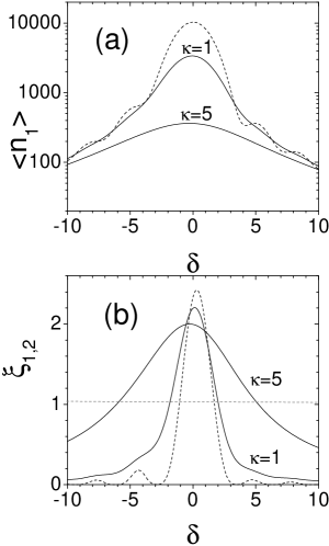
Figure 4: Semi-classical regime with $\gamma=0$: $\langle\hat{n}_{1}\rangle$, (a), and $\xi_{1,2}$, (b), vs. $\delta$ for $\rho=100$, $\tau=2$, $\kappa=0$ (dashed line), $1$ and $5$.

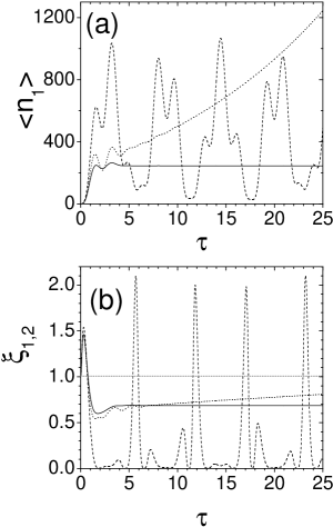
Figure 5: Semi-classical regime for $\rho=100$ and $\delta=3.5$: $\langle\hat{n}_{1}\rangle$, (a), and $\xi_{1,2}$, (b), vs. $\tau$ for $\gamma=0$, $\kappa=0$ (dashed line), for $\gamma=0.2$, $\kappa=0$ (dotted line) and for $\gamma=\kappa=0.5$ (continuous line).

Figures 3 and 4 show the effect of losses, in the semi-classical regime, on the atomic population $\langle\hat{n}_{1}\rangle$, (a), and on the number squeezing parameter $\xi_{1,2}$, (b), plotted as a function of $\delta$ for $\rho=100$ and $\tau=2$. Fig.3 shows the effect of the atomic decoherence on the the high-Q cavity regime ($\kappa=0$) for $\gamma=0$ (dashed line), $0.5$ and $1$. We observe that increasing $\gamma$ the population of the mode 1 decreases and the number squeezing parameter $\xi_{1,2}$ increases in the region of detuning where is less than one, i.e. where atom-atom number squeezing occurs. A similar behavior can be observed increasing the radiation losses in the semi-classical regime, as shown in fig.4, where $\langle\hat{n}_{1}\rangle$, (a), and $\xi_{1,2}$, (b), are plotted vs. $\delta$ for $\gamma=0$, $\kappa=0,1,5$ and $\rho=100$. In both the cases, in order to observe number squeezing in the semi-classical regime, it is necessary to detune the probe field from resonance, as it was already pointed out in ref.PRA . The inclusion of losses allows also to reach a steady-state regime when the gain $g$ is negative. In this case, the covariance matrix $\mathbf{C}(\infty)=\mathbf{Q}(\infty)$ becomes asymptotically constant. An example of this behavior is shown in fig.5, where $\langle\hat{n}_{1}\rangle$, (a), and $\xi_{1,2}$, (b), are plotted vs. $\tau$ for $\rho=100$ and $\delta=3.5$. The dashed line shows the ideal case $\gamma=\kappa=0$: because $g^{(0)}=0$ (as it can be observed from fig.1), the solution is oscillating and the two atomic modes 1 and 2 are periodically number squeezed. The dotted line of fig.5 shows the case with $\kappa=0$ and $\gamma=0.2$. Here, $g=0.025$ and both the average population and the number squeezing parameter grow in time. Finally, the continuous line of fig.5 shows the case $\gamma=\kappa=0.5$: the gain is $g=-0.5$ and the system reaches a stationary state in which $\xi_{1,2}=0.7$. This case is of some interest because a steady-state atom-atom number squeezed state is obtained in a linear system.

Let now consider the effect of losses on the quantum regime. Fig.6 shows the average population $\langle\hat{n}_{1}\rangle$, (a), and the atom-photon number squeezing parameter $\xi_{1,3}$, (b), as a function of $\tau$ for $1/\rho=\delta=5$. Dashed lines in fig.6 a and b are for $\kappa=\gamma=0$, the dotted lines are for $\kappa=0$ and $\gamma=0.15$ and the continuous lines are for $\kappa=\gamma=0.15$. We note that the atomic decoherence (i.e. $\gamma$) causes a drastic reduction of the number-squeezing between atoms and photons. However, choosing $\gamma=\kappa<g^{(0)}$ (where $g^{(0)}<\sqrt{\rho/2}$), we may keep $\xi_{1,3}$ constant and less than one for a relatively long time, like in the ideal case case without losses. Notice that in the quantum regime the below-threshold regime (i.e. $g<\gamma$) is not of interest because the average number of quanta generated in each modes remains less than one.

IV.3 Superradiant regime

In this section we present analytical results for the superradiant regime in the asymptotic limit $|{\rm Im}\omega_{1}|\tau\gg 1$, where $\omega_{1}$ is the unstable root of Eq.(27) with negative imaginary part. For $\kappa\gg|\omega_{1}|$ and assuming for simplicity $\gamma=0$, one root of Eq.(27) can be discharged as it decays to zero as $\exp{(-\kappa\tau)}$ and the other two roots may be obtained solving the following quadratic equation:

$$\omega^{2}+\frac{\omega+\delta+i\kappa}{(\delta+i\kappa)^{2}-1/\rho^{2}}-\frac{1}{\rho^{2}}=0.$$ (28)

From Eq.(28) it is possible to calculate explicitly the unstable root and evaluate asymptotically the expressions of the function $f_{ij}$ appearing in Eq.(13). From them, it is possible to evaluate the expectation values of the occupation numbers in the semi-classical and quantum regimes.

IV.3.1 Semi-classical limit of the superradiant regime

For $\kappa^{3/2}>1\gg\sqrt{\kappa}/\rho$ and $\delta=0$, the solutions of Eq.(28) are $\omega_{1,2}=\approx(1\mp i)/\sqrt{2\kappa}$ and the average occupation numbers are:

$$\langle n_{1}\rangle \approx \frac{\rho^{2}}{16\kappa}\left[1+\frac{\sqrt{2\kappa}}{\rho}\right]e^{(2/\kappa)^{1/2}\tau}$$ (29)

$$\langle n_{2}\rangle \approx \frac{\rho^{2}}{16\kappa}e^{(2/\kappa)^{1/2}\tau}$$ (30)

$$\langle n_{3}\rangle \approx \frac{\rho}{8\kappa^{2}}e^{(2/\kappa)^{1/2}\tau}$$ (31)

We observe that $\langle n_{1}\rangle\approx\langle n_{2}\rangle$ and $\langle n_{3}\rangle\approx(2/\rho\kappa)\langle n_{1}\rangle\ll\langle n_{1}\rangle$, so that the number of emitted photons is much smaller than the number of atoms in the two motional states. The asymptotic expression of the expectation value (26) of the bunching parameter is

$$\langle\hat{B}^{\dagger}\hat{B}\rangle\approx\frac{1}{4N}\left[1+\frac{\sqrt{2\kappa}}{\rho}\right]e^{(2/\kappa)^{1/2}\tau}.$$ (32)

Assuming that $\langle\hat{B}^{\dagger}\hat{B}\rangle$ approaches a maximum value of the order of one, then the maximum average number of emitted photons is about $\rho N/2\kappa^{2}$, whereas the maximum fraction of atoms gaining a momentum $2\hbar k_{p}$ is about $\rho^{2}/4\kappa$.

IV.3.2 Quantum limit of the superradiant regime

For $\kappa^{3/2}\gg 1>\rho/\sqrt{\kappa}$ and $\delta=1/\rho$, the solutions of Eq.(28) are $\omega_{1,2}\approx 1/\rho\mp i\rho/(2\kappa)$ and the average occupation numbers are:

$$\langle n_{1}\rangle \approx \left[1+\left(\frac{\rho}{\sqrt{2\kappa}}\right)^{4}\right]e^{(\rho/\kappa)\tau}$$ (33)

$$\langle n_{2}\rangle \approx \left(\frac{\rho}{2\sqrt{\kappa}}\right)^{4}e^{(\rho/\kappa)\tau}$$ (34)

$$\langle n_{3}\rangle \approx \frac{\rho}{2\kappa^{2}}e^{(\rho/\kappa)\tau}.$$ (35)

In this case, $\langle n_{2,3}\rangle\ll\langle n_{1}\rangle$ and $\langle n_{2}\rangle\approx(\rho/2)^{3}\langle n_{3}\rangle$: the average number of emitted photons is much less than the average number of atoms scattering a photon from the pump to the probe. Furthermore, the number of atoms making the reverse process, i.e. scattering a photon from the probe to the pump, can be larger than the number of photons scattered into the probe mode if $\rho>2$, as it occurs in the current experiment on BEC superradiance MIT ; LENS . In this regime the asymptotic expression of the expectation value of the bunching parameter is:

$$\langle\hat{B}^{\dagger}\hat{B}\rangle\approx\frac{1}{N}\left[1+\frac{1}{2}\left(\frac{\rho}{\sqrt{2\kappa}}\right)^{4}\right]e^{(\rho/\kappa)\tau},$$ (36)

so that $\langle n_{3}\rangle\approx(\rho N/2\kappa^{2})\langle\hat{B}^{\dagger}\hat{B}\rangle$, as in the semi-classical limit. The only difference is that in the quantum regime the maximum of $\langle\hat{B}^{\dagger}\hat{B}\rangle$ is $1/2$, so that the maximum number of scattered photon in the quantum limit is half of that obtained in the semi-classical limit.

V Entanglement and separability

In this Section we analyze the kind of entanglement that can be generated from our system. First, we establish notation and illustrate the separability criteria. We also apply the criteria to the state obtained in the ideal dynamics. Then, we address the effects of losses. We study both the separability properties of the tripartite state resulting from the evolution from the vacuum, as well as of the three two-mode states that are obtained by partial tracing over one of the modes. The basis of our analysis is that both the tripartite state and the partial traces are Gaussian states at any time. Therefore, we are able to fully characterize three-mode and two-mode entanglement as a function of the interaction parameters simon ; Giedke .

V.1 Three-mode entanglement

Concerning entanglement properties, three-mode states may be classified as follows Giedke :

• : fully inseparable states, i.e. not separable for any grouping of the modes;

• : one-mode biseparable states, which are separable if two of the modes are grouped together, but inseparable with respect to the other groupings;

• : two-mode biseparable states, which are separable with respect to two of the three possible bipartite groupings but inseparable with respect to the third;

• : three-mode biseparable states, which are separable with respect to all three bipartite groupings, but cannot be written as a product state;

• : fully separable states, which can be written as a three-mode product state.

Separability properties are determined by the characteristic function. In order to simplify the analysis we rewrite the characteristic function (7) in terms of the real variables ${\mathbf{x}}^{T}\equiv(x_{1},x_{2},x_{3},y_{1},y_{2},y_{3})$ with $\xi_{j}=2^{-1/2}(y_{j}-ix_{j})$, $j=1,2,3$. We have

$$\chi({\mathbf{x}})=\exp\left\{-\frac{1}{4}{\mathbf{x}}^{T}{\mathbf{V}}{\mathbf{x}}\right\}\;,$$ (37)

where

$${\mathbf{V}}=2{\mathbf{\Lambda}}_{0}\left(\begin{array}[]{cc}{\mathbf{A}}&-{\mathbf{B}}\\ {\mathbf{B}}&{\mathbf{A}}\end{array}\right)\>{\mathbf{\Lambda}}_{0}\;,$$ (38)

with ${\mathbf{\Lambda}}_{0}=\hbox{Diag}(-1,1,1,1,1,1)$ and

$${\mathbf{A}}=\Re{\it e}\>{\mathbf{C}}\qquad{\mathbf{B}}=\Im{\it m}\>{\mathbf{C}}\;,$$ (39)

and where we omitted the explicit time dependence of the matrices. The entanglement properties of the three-mode state are determined by the positivity of the matrices

$$\Gamma_{j}=\Lambda_{j}{\mathbf{V}}\Lambda_{j}-i{\mathbf{J}}\qquad j=1,2,3$$

where $\Lambda_{1}=\hbox{Diag}(1,1,1,-1,1,1)$, $\Lambda_{2}=\hbox{Diag}(1,1,1,1,-1,1)$, $\Lambda_{3}=\hbox{Diag}(1,1,1,1,1,-1)$ and ${\mathbf{J}}$ is the symplectic block matrix

$${\mathbf{J}}=\left(\begin{array}[]{cc}0&-{\mathbf{I}}\\ {\mathbf{I}}&\quad 0\end{array}\right)\>,$$ (42)

${\mathbf{I}}$ being the $3\times 3$ identity matrix. The positivity of the matrix $\Gamma_{j}$ indicates that the $j$-th mode may be factorized from the other two. Therefore, we have that i) if $\Gamma_{j}<0$ $\forall j$ the state is in class 1; ii) if only one of the $\Gamma_{j}$ is positive the state is in class 2; iii) is only two of the $\Gamma_{j}$ are positive the state is in class 3; iv) if $\Gamma_{j}>0$, $\forall j$ then the state is either in class 4 or in class 5.

The covariance matrix ${\mathbf{V}}$ can be written as

$${\mathbf{V}}=\left(\begin{array}[]{cccccc}{\cal G}&-{\cal A}&-{\cal B}&0&{\cal D}&{\cal E}\\ -{\cal A}&{\cal H}&{\cal C}&{\cal D}&0&-{\cal F}\\ -{\cal B}&{\cal C}&{\cal I}&{\cal E}&{\cal F}&0\\ 0&{\cal D}&{\cal E}&{\cal G}&{\cal A}&{\cal B}\\ {\cal D}&0&{\cal F}&{\cal A}&{\cal H}&{\cal C}\\ {\cal E}&-{\cal F}&0&{\cal B}&{\cal C}&{\cal I}\\ \end{array}\right)\;,$$ (43)

where

$${\cal A}=2\>\Re{\it e}\>C_{12}\quad {\cal D}=2\>\Im{\it m}\>C_{12}\quad {\cal G}=2\langle\hat{n}_{1}\rangle+1$$

$${\cal B}=2\>\Re{\it e}\>C_{13}\quad {\cal E}=2\>\Im{\it m}\>C_{13}\quad {\cal H}=2\langle\hat{n}_{2}\rangle+1$$ (44)

$${\cal C}=2\>\Re{\it e}\>C_{23}\quad {\cal F}=2\>\Im{\it m}\>C_{23}\quad {\cal I}=2\langle\hat{n}_{3}\rangle+1\;$$

and the matrix elements $C_{ij}$ are reported in Appendix B. Let us first consider the ideal case, when no losses are present. In this case we can prove analytically that the evolved state (3) is fully inseparable. In fact, we have that

$${\cal A}=2\sqrt{\langle\hat{n}_{2}\rangle(1+\langle\hat{n}_{1}\rangle)}\cos\phi_{2}\quad {\cal D}=2\sqrt{\langle\hat{n}_{2}\rangle(1+\langle\hat{n}_{1}\rangle)}\sin\phi_{2}$$

$${\cal B}=2\sqrt{\langle\hat{n}_{3}\rangle(1+\langle\hat{n}_{1}\rangle)}\cos\phi_{3}\quad {\cal E}=2\sqrt{\langle\hat{n}_{3}\rangle(1+\langle\hat{n}_{1}\rangle)}\sin\phi_{3}$$

$${\cal C}=2\sqrt{\langle\hat{n}_{2}\rangle\langle\hat{n}_{3}\rangle}\cos(\phi_{3}-\phi_{2})\quad {\cal F}=2\sqrt{\langle\hat{n}_{2}\rangle\langle\hat{n}_{3}\rangle}\sin(\phi_{3}-\phi_{2})\;,$$ (45)

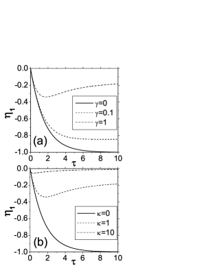
Figure 10: Quantum regime for $\rho=0.2$ and $\delta=5$: minimum eigenvalue of matrix $\Gamma_{1}$ (or $\Gamma_{3}$, see the text) for $\kappa=0$ and different values of $\gamma$ (a) and for $\gamma=0$ and different values of $\kappa$ (b).

from which, in turn, it is straightforward to prove that the minimum eigenvalues of the matrices $\Gamma_{j}$ are always negative. In the non ideal case, when $\gamma$ or $\kappa$ are different from zero, the expressions given in Eqs. (44) and accordingly the minimum eigenvalues of matrices $\Gamma_{j}$ should be calculated numerically. In Fig. 7, 8 and 9 the minimum eigenvalues of matrices $\Gamma_{1}$, $\Gamma_{2}$ and $\Gamma_{3}$ are plotted in the semi-classical regime, with $\rho=100$. In this regime we can observe that modes $1$ and $2$ remain non separable from the three mode state even for large values of atomic decoherence $\gamma$ and radiation losses $\kappa$. Instead inseparability of mode $3$ is not so robust especially in presence of some atomic decoherence. In Fig. 10 and 11 the minimum eigenvalues of matrices $\Gamma_{1}$ and $\Gamma_{2}$ are plotted in the quantum regime, with $\rho=0.2$. The minimum eigenvalue of the matrix $\Gamma_{3}$ is not reported in the figure since the behavior is similar to that of $\Gamma_{1}$. In this regime we can observe that modes $1$ and $3$ remain non separable from the three mode state even for large values of atomic decoherence $\gamma$ and radiation losses $\kappa$. Instead inseparability of mode $2$ is very sensible especially in presence of some radiation losses. In any case in the quantum regime the three eigenvalues increasing $\gamma$ and $\kappa$ approaches to zero but remain negative. In the semi-classical regime the eigenvalue of $\Gamma_{3}$ that corresponds to photonic mode $3$ becomes positive increasing $\gamma$.

V.2 Two-mode entanglement

In experimental conditions where only two of the modes are available for investigations, the relevant piece of information is contained in the partial traces of the global three-mode state. Therefore, besides the study of three-mode entanglement it is also of interest to analyze the two-mode entanglement properties of partial traces. At first we notice that the Gaussian character of the state is preserved by the partial trace operation. Moreover, the covariance matrices $V_{ij}$ of three possible partial traces $\hat{\varrho}_{ij}=\hbox{Tr}_{k}[\hat{\varrho}]$, $i\neq j\neq k$ can be obtained from ${\mathbf{V}}$ by deleting the corresponding $k$-th and $k+3$-th rows and columns. The Gaussian character of the partial traces also permits to check separability using the necessary and sufficient conditions introduced in Ref. simon , namely by the positivity of the matrices ${\mathbf{S}}_{ij}$ and ${\mathbf{S}}_{ij}^{\prime}$ that are obtained by deleting the $k$-th and $k+3$-th rows and columns either from $\Gamma_{i}$ or $\Gamma_{j}$. Since they differ only for the sign of some off-diagonal elements it is easy to prove that they have the same eigenvalues. Therefore, we employ only ${\mathbf{S}}_{ij}$ in checking separability. The matrices ${\mathbf{S}}_{ij}$ are given by

$${\mathbf{S}}_{12} = \left(\begin{array}[]{cccc}{\cal G}&-{\cal A}&i&{\cal D}\\ -{\cal A}&{\cal H}&-{\cal D}&i\\ -i&-{\cal D}&{\cal G}&-{\cal A}\\ {\cal D}&-i&-{\cal A}&{\cal H}\end{array}\right)$$ (50)

$${\mathbf{S}}_{13} = \left(\begin{array}[]{cccc}{\cal G}&-{\cal B}&i&{\cal E}\\ -{\cal B}&{\cal L}&-{\cal E}&i\\ -i&-{\cal E}&{\cal G}&-{\cal B}\\ {\cal E}&-i&-{\cal B}&{\cal I}\end{array}\right)$$ (55)

$${\mathbf{S}}_{23} = \left(\begin{array}[]{cccc}{\cal H}&{\cal C}&i&-{\cal F}\\ {\cal C}&{\cal L}&-{\cal L}&i\\ -i&-{\cal L}&{\cal H}&-{\cal C}\\ -{\cal F}&-i&-{\cal C}&{\cal I}\end{array}\right)\;.$$ (60)

In ideal conditions with $\gamma=\kappa=0$ the minimum eigenvalues of ${\mathbf{S}}_{1k}$, $k=2,3$ are given by

$$\eta_{1k}=\langle\hat{n}_{1}\rangle+\langle\hat{n}_{k}\rangle-\sqrt{4\langle\hat{n}_{k}\rangle+(\langle\hat{n}_{1}\rangle+\langle\hat{n}_{k}\rangle)^{2}}$$ (61)

and thus are always negative. On the contrary, the minimum eigenvalue of $S_{23}$ is given by

$$\eta_{23}=1+\langle\hat{n}_{1}\rangle+\sqrt{(1+\langle\hat{n}_{1}\rangle)^{2}-4\langle\hat{n}_{k}\rangle}$$ (62)

where $\langle\hat{n}_{k}\rangle={\rm max}(\langle\hat{n}_{2}\rangle,\langle\hat{n}_{3}\rangle)$. Note that $\eta_{23}$ is always positive. Therefore, after partial tracing we may have atom-atom entanglement (entanglement between mode $a_{1}$ and mode $a_{2}$) or scattered atom-radiation entanglement (entanglement between mode $a_{1}$ and mode $a_{3}$) but no entanglement between mode $a_{2}$ and mode $a_{3}$.

For $\tau\gg 1$ we know the asymptotic expressions for populations in the ideal case without losses PRA , so we can obtain the stationary value of $\eta_{1k}$ as

$$\eta_{1k}\approx-\frac{2\langle\hat{n}_{k}\rangle}{\langle\hat{n}_{1}\rangle+\langle\hat{n}_{k}\rangle}.$$ (63)

In the high-gain semi-classical regime ($\rho\gg 1$) PRA ,

$$\langle\hat{n}_{1}\rangle \approx \frac{1}{18}\left[\frac{\rho^{2}}{2}+\rho\right]e^{\sqrt{3}\tau},$$ (64)

$$\langle\hat{n}_{2}\rangle \approx \frac{\rho^{2}}{36}e^{\sqrt{3}\tau},$$ (65)

$$\langle\hat{n}_{3}\rangle \approx \frac{\rho}{18}e^{\sqrt{3}\tau},$$ (66)

so that

$$\eta_{12}\approx-\frac{\rho}{1+\rho}\qquad\eta_{13}\approx-\frac{4}{4+\rho}$$ (67)

In the high-gain quantum regime ($\rho<1$),

$$\langle n_{1}\rangle \approx \frac{1}{4}\left[1+\left(\frac{\rho}{2}\right)^{3}\right]e^{\sqrt{2\rho}\tau},$$ (68)

$$\langle n_{2}\rangle \approx \frac{1}{4}\left(\frac{\rho}{2}\right)^{3}e^{\sqrt{2\rho}\tau},$$ (69)

$$\langle n_{3}\rangle \approx \frac{1}{4}e^{\sqrt{2\rho}\tau},$$ (70)

so that

$$\eta_{12}\approx-\frac{\rho^{3}}{4+\rho^{3}}\qquad\eta_{13}\approx-\frac{16}{16+\rho^{3}}.$$ (71)

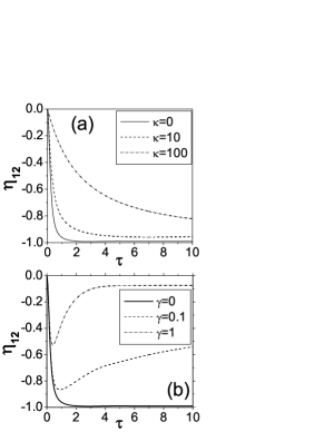
Figure 12: Semi-classical regime for $\rho=100$ and $\delta=0$: minimum eigenvalue of matrix $S_{12}$ for $\kappa=0$ and different values of $\gamma$ (a) and for $\gamma=0$ and different values of $\kappa$ (b).

In the non ideal case, when $\gamma$ or $\kappa$ are different from zero, the minimum eigenvalues of matrices $S_{12}$ and $S_{13}$ can be easily obtained numerically. In Fig. 12 and 13 the minimum eigenvalues of matrices $S_{12}$, $S_{13}$ are plotted for the semi-classical regime. We can observe that the atom-atom entanglement of the reduced state $12$ is robust, as the minimum eigenvalue remain negative increasing atomic decoherence $\gamma$ and radiation losses $\kappa$. On the contrary atom-photon entanglement of the reduced state $13$ is more sensitive to noise: the eigenvalue remains negative increasing $\kappa$ and become positive in presence of some atomic decoherence.

In Fig. 14 and 15 are plotted the minimum eigenvalues of matrices $S_{12}$, $S_{13}$ in the quantum regime, with $\rho=0.2$. Here the atom-photon entanglement in the state $13$ is robust while atom-atom entanglement of the state $12$ is not. The minimum eigenvalue always remains negative, but it starts from a very small absolute value and approaches very fast to zero increasing $\kappa$ and $\gamma$.

VI Conclusions

We have investigated how cavity radiation losses and atomic decoherence influence the generation of two (atom-atom or atom-radiation) and three mode entanglement in the collective atomic recoil lasing (CARL) by a Bose-Einstein condensate driven by a far off-resonant pump laser. The atoms back-scatter photons from the pump to a weak radiation mode circulating in a ring cavity, recoiling with opposite momentum $\pm 2\hbar k_{p}$ along the ring cavity axis. Our analysis has been focused to the linear regime, in which the ground state of the condensate remains approximately undepleted and the dynamics is described by three parametrically coupled boson operators, corresponding to the radiation mode and two condensates with momentum displaced by $\pm\ 2\hbar\vec{k}_{p}$. The problem resembles that of three optical modes generated in a $\chi^{(2)}$ medium opa and thus our results may have a more general interest also behind the physics of the BEC. We have solved analytically the dissipative Master equation in terms of the Wigner function and we have investigated the entanglement properties of the evolved state. We found that three-mode entanglement as well two-mode atom-atom and atom-photon entanglement is generally robust against cavity losses and decoherence. The analysis has been focused of the different dynamical regimes, the high-Q cavity regime, with low cavity losses, and the superradiant regime in the so-called ’bad-cavity limit’. We have found that entanglement in the high-Q cavity regime is generally robust against either cavity or decoherence losses. On the contrary, losses seriously limit atom-atom and atom-radiation number squeezing production in CARL Gasenzer . Concerning the superradiant regime, atom-atom entanglement in the semi-classical limit is generally more robust than atom-radiation entanglement in the quantum-limit. Finally, we have proved that the state generated in the ideal case without losses is fully inseparable. We conclude that the present system is a good candidate for the experimental observation of entanglement in condensate systems since, in particular, steady-state entanglement may be obtained both between atoms with opposite momenta and between atoms and photons.

Appendix A Solution of the Fokker-Planck equation

In order to solve Eq.(8) for the Green function $G(\mathbf{u},t;\mathbf{u}_{0},0)$ it is helpful to first perform a similarity transformation to diagonalize the drift matrix $\mathbf{A}$:

$$\tilde{\mathbf{A}}=\mathbf{S}\mathbf{A}\mathbf{S}^{-1}=\mbox{diag}\{\lambda_{1}\lambda_{2}\lambda_{3}\},$$ (72)

where the complex eigenvalues $\lambda_{j}$ of $\mathbf{A}$ (with $j=1,2,3$) are obtained from the characteristic equation

$$\det(\mathbf{A}-\lambda\mathbf{I})=0,$$ (73)

$\mathbf{I}$ is the $3\times 3$ identity matrix and the columns of $\mathbf{S}^{-1}$ are the right eigenvectors of $\mathbf{A}$ with $\det(\mathbf{S})=1$. Solving Eq.(73) we obtain $\lambda_{j}=i(\omega_{j}-\delta)-\gamma_{+}$, where $\omega_{j}$ are the three roots of the cubic equation (15), whereas the eigenvectors of $\mathbf{A}$ corresponding to the $j$-th eigenvalue are

$$\mathbf{a}_{j}^{T}={\cal N}_{j}\left(i\sqrt{\frac{\rho}{2}}\left(\omega_{j}+\beta\right),-i\sqrt{\frac{\rho}{2}}\left(\omega_{j}-\beta\right),-\omega_{j}^{2}+\beta^{2}\right),$$ (74)

where $\beta=1/\rho+i\gamma_{-}$ and

$${\cal N}_{1}=\frac{1}{\omega_{2}-\omega_{3}}\;\;\;\;{\cal N}_{2}=\frac{1}{\omega_{1}-\omega_{3}}\;\;\;\;{\cal N}_{3}=\frac{1}{\omega_{1}-\omega_{2}}.$$ (75)

Explicitly calculating the inverse matrix of $S^{-1}$ we have

$$\mathbf{S}=\left(\begin{array}[]{rrr}i\sqrt{\rho/2}\;(a_{22}a_{23}/{\cal N}_{1})&i\sqrt{\rho/2}\;(a_{12}a_{13}/{\cal N}_{1})&-{\cal N}_{2}{\cal N}_{3}/{\cal N}_{1}\\ -i\sqrt{\rho/2}\;(a_{23}a_{21}/{\cal N}_{2})&-i\sqrt{\rho/2}\;(a_{11}a_{13}/{\cal N}_{2})&{\cal N}_{1}{\cal N}_{3}/{\cal N}_{2}\\ i\sqrt{\rho/2}\;(a_{21}a_{22}/{\cal N}_{3})&i\sqrt{\rho/2}\;(a_{12}a_{11}/{\cal N}_{3})&-{\cal N}_{1}{\cal N}_{2}/{\cal N}_{3},\end{array}\right)$$ (76)

where $a_{ij}=(\mathbf{a}_{j})_{i}$. Now we transform the Fokker-Plank equation (8) in the new variable $\mathbf{v}\equiv\mathbf{S}\mathbf{u}$. From (72) we obtain

$$\mathbf{u}^{\prime T}\mathbf{A}\mathbf{u} = \mathbf{u}^{\prime T}(\mathbf{S}^{-1}\tilde{\mathbf{A}}\mathbf{S})\mathbf{u}=\mathbf{v}^{\prime T}\tilde{\mathbf{A}}\mathbf{v}$$ (77)

$$\mathbf{u}^{\prime T}\mathbf{D}\mathbf{u}^{\prime*} = (\mathbf{v}^{\prime T}\mathbf{S})\mathbf{D}(\mathbf{S}^{T}\mathbf{v}^{\prime})^{*}=\mathbf{v}^{\prime T}\tilde{\mathbf{D}}\mathbf{v}^{\prime*},$$ (78)

where $\tilde{\mathbf{D}}\equiv\mathbf{S}\mathbf{D}\mathbf{S}^{{\dagger}}$, $\mathbf{S}^{{\dagger}}=(\mathbf{S}^{T})^{*}$ and $\mathbf{v}^{\prime T}=\mathbf{u}^{\prime T}\mathbf{S}^{-1}$. Using (77) and (78) Eq. (8) becomes

$$\frac{\partial\tilde{W}}{\partial\tau}=-\left(\textbf{v}^{\prime T}\mathbf{\tilde{A}}\textbf{v}+{\rm c.c.}\right)\tilde{W}+\textbf{v}^{\prime T}\tilde{\mathbf{D}}\textbf{v}^{\prime*}\tilde{W},$$ (79)

where $\tilde{W}(\mathbf{v},\tau)=W(\mathbf{S}^{-1}\mathbf{v},\tau)$. Eq.(79) is a linear Fokker-Plank equation with diagonal drift. Introducing the Fourier transform

$$\tilde{U}(\mathbf{k},\tau)=\int\frac{d^{2}\mathbf{k}}{\pi^{3}}\tilde{W}(\mathbf{v})\exp(\mathbf{k}^{*T}\mathbf{v}-\mathbf{k}^{T}\mathbf{v}^{*}),$$ (80)

Eq.(79) becomes

$$\frac{\partial\tilde{U}}{\partial\tau}=\left(\mathbf{k}^{*T}\mathbf{\tilde{A}}\mathbf{k}^{\prime*}+\mathbf{k}^{T}\mathbf{\tilde{A}}^{*}\mathbf{k}^{\prime}\right)\tilde{U}-\left(\mathbf{k}^{*T}\tilde{\mathbf{D}}\mathbf{k}\right)\tilde{U}.$$ (81)

where

$$\textbf{k}^{T}=\left(k_{1},k_{2},k_{3}\right)\qquad\mathbf{k}^{\prime T}=\left(\frac{\partial}{\partial k_{1}},\frac{\partial}{\partial k_{2}},\frac{\partial}{\partial k_{3}}\right).$$ (82)

The Fourier transform of initial condition of the Green function $\tilde{G}(\mathbf{v},0;\mathbf{S}\mathbf{u}_{0},0)=\delta^{3}(\mathbf{v}-\mathbf{S}\mathbf{u}_{0})$ is

$$\tilde{U}(\mathbf{k},0)=\exp\left[\mathbf{k}^{*T}\mathbf{S}\mathbf{u}_{0}-\mathbf{k}^{T}(\mathbf{S}\mathbf{u}_{0})^{*}\right].$$ (83)

Eq.(81) is now solved using the method of the characteristics. Since $\tilde{\mathbf{A}}$ is diagonal the subsidiary equations are

$$\frac{d\tau}{1}=\frac{dk^{*}_{1}}{-\lambda_{1}k^{*}_{2}}=\frac{dk^{*}_{2}}{-\lambda_{2}k^{*}_{2}}=\frac{dk^{*}_{3}}{-\lambda_{3}k^{*}_{3}}=\frac{d\tilde{U}}{(-\mathbf{k}^{*T}\tilde{\mathbf{D}}\mathbf{k})\tilde{U}}$$ (84)

and have solutions

$$\mathbf{k}=e^{-\tilde{\mathbf{A}}^{*}\tau}\mathbf{c}={\rm constant}.$$ (85)

Then

$$\frac{d\tilde{U}}{\tilde{U}}=-\mathbf{k}^{*T}\tilde{\mathbf{D}}\mathbf{k}d\tau=-\mathbf{c}^{*T}\left(e^{-\tilde{\mathbf{A}}\tau}\tilde{\mathbf{D}}e^{-\tilde{\mathbf{A}}^{*}\tau}\right)\mathbf{c}d\tau=-\mathbf{c}^{*T}\left[\tilde{\mathbf{D}}_{ij}e^{-(\lambda_{i}+\lambda_{j}^{*})\tau}\right]\mathbf{c}d\tau,$$ (86)

where $(\mathbf{B}_{ij})$ denotes the matrix with elements $\mathbf{B}_{ij}$, and we find, using Eq. (85),

$$\ln\tilde{U}=\mathbf{k}^{*T}\left\{\frac{\tilde{\mathbf{D}}_{ij}}{\lambda_{i}+\lambda_{j}^{*}}\left[1-e^{(\lambda_{i}+\lambda_{j}^{*})\tau}\right]\right\}\mathbf{k}+\mbox{constant}\>.$$ (87)

It follows that

$$\tilde{U}\exp\left\{\mathbf{k}^{*T}\tilde{\mathbf{Q}}\mathbf{k}\right\}=\mbox{constant},$$ (88)

where $\tilde{\mathbf{Q}}$ is the $3\times 3$ matrix with elements

$$\tilde{\mathbf{Q}}_{ij}\equiv-\frac{\tilde{D}_{ij}}{\lambda_{i}+\lambda_{j}^{*}}\left[1-e^{(\lambda_{i}+\lambda_{j}^{*})\tau}\right]=\int_{0}^{\tau}d\tau^{\prime}\tilde{D}_{ij}e^{(\lambda_{i}+\lambda_{j}^{*})\tau^{\prime}}.$$ (89)

Thus, from Eqs. (85) and (88), the solution for $\tilde{U}$ takes the general form

$$\tilde{U}(\mathbf{k},\tau)=\Phi(e^{\tilde{\mathbf{A}}^{*}\tau}\mathbf{k})\exp\{-\mathbf{k}^{*T}\tilde{\mathbf{Q}}\mathbf{k}\}$$ (90)

where $\Phi$ is an arbitrary function. Choosing $\Phi$ to match the initial condition (83), we find

$$\tilde{U}(\mathbf{k},\tau)=\exp\left\{\mathbf{k}^{*T}(\mathbf{S}e^{\mathbf{A}\tau}\mathbf{u}_{0})-\mathbf{k}^{T}(\mathbf{S}e^{\mathbf{A}\tau}\mathbf{u}_{0})^{*}\right\}\exp\left\{-\mathbf{k}^{*T}\tilde{\mathbf{Q}}\mathbf{k}\right\}.$$ (91)

In the argument of the first exponential on the right-hand side we have used (72) to write $\exp(\tilde{\mathbf{A}}\tau)\mathbf{S}=\mathbf{S}\exp(\mathbf{A}\tau)$. Inverting the Fourier transform we obtain

$$\tilde{G}(\mathbf{v},\tau;\mathbf{S}\mathbf{u}_{0},0)=\frac{1}{\pi^{3}\det\mathbf{\tilde{Q}}}\exp\left\{\left(\mathbf{v}-\mathbf{S}e^{\mathbf{A}\tau}\mathbf{u}_{0}\right)^{\dagger}\mathbf{\tilde{Q}}^{-1}\left(\mathbf{v}-\mathbf{S}e^{\tilde{\mathbf{A}}\tau}\mathbf{u}_{0}\right)\right\}$$ (92)

and so transforming back the variables

$$G(\mathbf{u},\tau;\mathbf{u}_{0},0)=\frac{1}{\pi^{3}\det\mathbf{Q}}\exp\left\{\left(\mathbf{u}-e^{\mathbf{A}\tau}\mathbf{u}_{0}\right)^{\dagger}\mathbf{Q}^{-1}\left(\mathbf{u}-e^{\mathbf{A}\tau}\mathbf{u}_{0}\right)\right\}.$$ (93)

where

$$\mathbf{Q}=\mathbf{S}^{-1}\hat{\mathbf{Q}}\left(\mathbf{S}^{-1}\right)^{\dagger}=\int_{0}^{\tau}d\tau^{\prime}e^{\mathbf{A}\tau^{\prime}}\mathbf{D}\left(e^{\mathbf{A}\tau^{\prime}}\right)^{\dagger}.$$ (94)

Appendix B Elements of the matrices ${\mathbf{M}}$, Eq. (13), and ${\mathbf{C}}$, Eq. (17)

The expressions of the functions $f_{ij}$ which appear as elements of the matrix $\mathbf{M}$, Eq. (13), are

$$f_{11}(\tau) = e^{-(\gamma_{+}+i\delta)\tau}\sum_{j=1}^{3}[(\omega_{j}-\alpha)(\omega_{j}+\beta)-\rho/2]\frac{e^{i\omega_{j}\tau}}{\Delta_{j}}$$ (95)

$$f_{22}(\tau) = e^{-(\gamma_{+}+i\delta)\tau}\sum_{j=1}^{3}[(\omega_{j}-\alpha)(\omega_{j}-\beta)+\rho/2]\frac{e^{i\omega_{j}\tau}}{\Delta_{j}}$$ (96)

$$f_{33}(\tau) = e^{-(\gamma_{+}+i\delta)\tau}\sum_{j=1}^{3}(\omega_{j}^{2}-\beta^{2})\frac{e^{i\omega_{j}\tau}}{\Delta_{j}}$$ (97)

$$f_{12}(\tau) = -\frac{\rho}{2}e^{-(\gamma_{+}+i\delta)\tau}\sum_{j=1}^{3}\frac{e^{i\omega_{j}\tau}}{\Delta_{j}}$$ (98)

$$f_{13}(\tau) = -i\sqrt{\frac{\rho}{2}}e^{-(\gamma_{+}+i\delta)\tau}\sum_{j=1}^{3}(\omega_{j}+\beta)\frac{e^{i\omega_{j}\tau}}{\Delta_{j}}$$ (99)

$$f_{23}(\tau) = i\sqrt{\frac{\rho}{2}}e^{-(\gamma_{+}+i\delta)\tau}\sum_{j=1}^{3}(\omega_{j}-\beta)\frac{e^{i\omega_{j}\tau}}{\Delta_{j}}$$ (100)

where $\alpha=\delta+i(\kappa-\gamma_{+})$, $\beta=1/\rho+i\gamma_{-}$, $\Delta_{j}=(\omega_{j}-\omega_{k})(\omega_{j}-\omega_{m})$ (with $j\neq k\neq m$) and $\omega_{1}$, $\omega_{2}$ and $\omega_{3}$ are the roots of the cubic Eq.(15). It is possible to show that $f_{ij}(0)=\delta_{ij}$ in order to satisfy the initial condition $\mathbf{M}(0)=\mathbf{I}$.

The explicit components of the covariance matrix

$$\mathbf{C}(\tau)=\mathbf{Q}(\tau)+\frac{1}{2}\mathbf{M}(\tau)\mathbf{M}^{{\dagger}}(\tau),$$

where $\mathbf{M}$ and $\mathbf{Q}$ are defined in (13) and (14), are

$$C_{11}(\tau) = \int_{0}^{\tau}d\tau^{\prime}\left\{\gamma_{1}|f_{11}|^{2}+\gamma_{2}|f_{12}|^{2}+\kappa|f_{13}|^{2}\right\}+\frac{1}{2}\left(|f_{11}|^{2}+|f_{12}|^{2}+|f_{13}|^{2}\right)$$ (101)

$$C_{22}(\tau) = \int_{0}^{\tau}d\tau^{\prime}\left\{\gamma_{1}|f_{12}|^{2}+\gamma_{2}|f_{22}|^{2}+\kappa|f_{23}|^{2}\right\}+\frac{1}{2}\left(|f_{12}|^{2}+|f_{22}|^{2}+|f_{23}|^{2}\right)$$ (102)

$$C_{33}(\tau) = \int_{0}^{\tau}d\tau^{\prime}\left\{\gamma_{1}|f_{13}|^{2}+\gamma_{2}|f_{23}|^{2}+\kappa|f_{33}|^{2}\right\}+\frac{1}{2}\left(|f_{13}|^{2}+|f_{23}|^{2}+|f_{33}|^{2}\right)$$ (103)

$$C_{12}(\tau) = \int_{0}^{\tau}d\tau^{\prime}\left\{-\gamma_{1}f_{11}f_{12}^{*}+\gamma_{2}f_{12}f_{22}^{*}+\kappa f_{13}f_{23}^{*}\right\}+\frac{1}{2}\left(-f_{11}f_{12}^{*}+f_{12}f_{22}^{*}+f_{13}f_{23}^{*}\right)$$ (104)

$$C_{13}(\tau) = \int_{0}^{\tau}d\tau^{\prime}\left\{\gamma_{1}f_{11}f_{13}^{*}-\gamma_{2}f_{12}f_{23}^{*}+\kappa f_{13}f_{33}^{*}\right\}+\frac{1}{2}\left(f_{11}f_{13}^{*}-f_{12}f_{23}^{*}+f_{13}f_{33}^{*}\right)$$ (105)

$$C_{23}(\tau) = \int_{0}^{\tau}d\tau^{\prime}\left\{-\gamma_{1}f_{12}f_{13}^{*}-\gamma_{2}f_{22}f_{23}^{*}+\kappa f_{23}f_{33}^{*}\right\}+\frac{1}{2}\left(-f_{12}f_{13}^{*}-f_{22}f_{23}^{*}+f_{23}f_{33}^{*}\right)$$ (106)

with $C_{ij}=C_{ji}^{*}$.

In the special case $\gamma_{+}=\gamma=\kappa$ and $\gamma_{-}=0$, $f_{ij}=e^{-\gamma\tau}f_{ij}^{(0)}$, where $f_{ij}^{(0)}$ is the solution without losses. As shown in Ref.PRA , they satisfy the following relations:

$$|f_{13}^{(0)}|^{2}+1 = |f_{23}^{(0)}|^{2}+|f_{33}^{(0)}|^{2}$$ (107)

$$|f_{11}^{(0)}|^{2}-1 = |f_{12}^{(0)}|^{2}+|f_{13}^{(0)}|^{2}$$ (108)

$$|f_{12}^{(0)}|^{2}+1 = |f_{22}^{(0)}|^{2}+|f_{23}^{(0)}|^{2}$$ (109)

$$f_{11}^{(0)}(f_{13}^{(0)})^{*} = -f_{12}^{(0)}(f_{23}^{(0)})^{*}+f_{13}^{(0)}(f_{33}^{(0)})^{*}$$ (110)

$$-f_{11}^{(0)}(f_{12}^{(0)})^{*} = f_{12}^{(0)}(f_{22}^{(0)})^{*}+f_{13}^{(0)}(f_{23}^{(0)})^{*}$$ (111)

$$-f_{12}^{(0)}(f_{13}^{(0)})^{*} = -f_{22}^{(0)}(f_{23}^{(0)})^{*}+f_{23}^{(0)}(f_{33}^{(0)})^{*}$$ (112)

Using Eqs.(107)-(109) in Eq.(101)-(103) and $C_{ii}=1/2+\langle{\hat{n}_{i}}\rangle$, we obtain that

$$\langle{\hat{n}_{1}}\rangle=\langle{\hat{n}_{2}}\rangle+\langle{\hat{n}_{3}}\rangle$$ (113)

and

$$\frac{d\langle{\hat{n}_{i}}\rangle}{d\tau}=\frac{d\langle{\hat{n}_{i}^{(0)}}\rangle}{d\tau}e^{-2\gamma\tau},$$ (114)

where $\langle{\hat{n}_{i}^{(0)}}\rangle$ are the expectation values of the occupation numbers of the three modes in the ideal case without losses.

Figure 1: Growth rate $g=-{\rm Im}\omega-\gamma$ vs. $\delta$ for the unstable root of the cubic equation (15) in the semi-classical limit, $\rho=100$. In (a) $\kappa=0$ and $\gamma=0.5,1,2$; in (b) $\gamma=0$ and $\kappa=1,5,10$. The dashed lines represent the case $\kappa=\gamma=0$.

Figure 2: Growth rate $g=-{\rm Im}\omega-\gamma$ vs. $\delta$ for the unstable root of the cubic equation (15) in the quantum limit. In (a), $\rho=0.2$, $\kappa=0$ and $\gamma=0.2,0.5,1$; in (b), $\rho=1$, $\gamma=0$ and $\kappa=0.5,1,5$. The dashed lines represent the case $\kappa=\gamma=0$.

Figure 3: Semi-classical regime with $\kappa=0$: $\langle\hat{n}_{1}\rangle$, (a), and $\xi_{1,2}$, (b), vs. $\delta$ for $\rho=100$, $\tau=2$, $\gamma=0$ (dashed line), $0.5$ and $1$.

Figure 6: Quantum regime for $1/\rho=\delta=5$: $\langle\hat{n}_{1}\rangle$, (a), and $\xi_{1,3}$, (b), vs. $\tau$ for $\gamma=0$, $\kappa=0$ (dashed line), for $\gamma=0.15$, $\kappa=0$ (dotted line) and for $\gamma=\kappa=0.15$ (continuous line).

Figure 7: Semi-classical regime for $\rho=100$ and $\delta=0.01$: minimum eigenvalue of matrix $\Gamma_{1}$ for $\kappa=0$ and different values of $\gamma$ (a) and for $\gamma=0$ and different values of $\kappa$ (b).

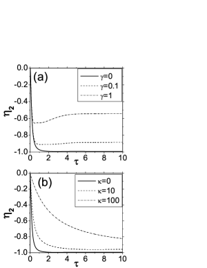
Figure 8: Semi-classical regime for $\rho=100$ and $\delta=0.01$: minimum eigenvalue of matrix $\Gamma_{2}$ for $\kappa=0$ and different values of $\gamma$ (a) and for $\gamma=0$ and different values of $\kappa$ (b).

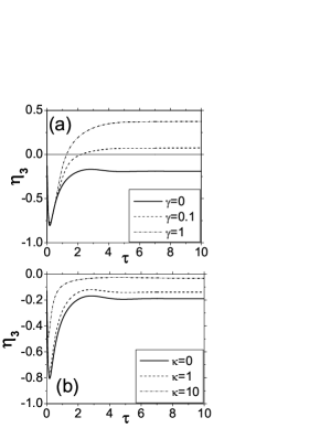
Figure 9: Semi-classical regime for $\rho=100$ and $\delta=0.01$: minimum eigenvalue of matrix $\Gamma_{3}$ for $\kappa=0$ and different values of $\gamma$ (a) and for $\gamma=0$ and different values of $\kappa$ (b).

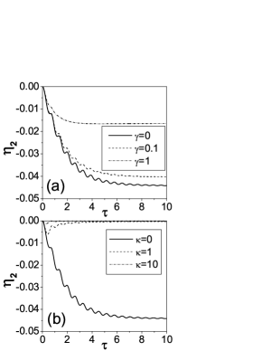
Figure 11: Quantum regime for $\rho=0.2$ and $\delta=5$: minimum eigenvalue of matrix $\Gamma_{2}$ for $\kappa=0$ and different values of $\gamma$ (a) and for $\gamma=0$ and different values of $\kappa$ (b).

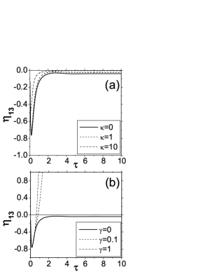
Figure 13: Semi-classical regime for $\rho=100$ and $\delta=0$: minimum eigenvalue of matrix $S_{13}$ for $\kappa=0$ and different values of $\gamma$ (a) and for $\gamma=0$ and different values of $\kappa$ (b).

Figure 14: Quantum regime for $\rho=0.2$ and $\delta=5$: minimum eigenvalue of matrix $S_{12}$ for $\kappa=0$ and different values of $\gamma$ (a) and for $\gamma=0$ and different values of $\kappa$ (b).

Figure 15: Quantum regime for $\rho=0.2$ and $\delta=5$: minimum eigenvalue of matrix $S_{13}$ for $\kappa=0$ and different values of $\gamma$ (a) and for $\gamma=0$ and different values of $\kappa$ (b).

References

- (1) P. Meystre, Atom Optics (Springer – Berlin), 2001.
- (2) R. Bonifacio and L. De Salvo Souza, Nucl. Instrum. and Meth. in Phys. Res. A 341, 360 (1994); R. Bonifacio, L. De Salvo Souza, L.M. Narducci and E.J. D’Angelo, Phys. Rev.A 50, 1716 (1994).
- (3) M.G. Moore and P. Meystre, Phys. Rev. A 58, 3248 (1998).
- (4) M.G. Moore, O. Zobay and P. Meystre, Phys. Rev. A 60, 1491 (1999).
- (5) N. Piovella, M. Cola, R. Bonifacio, Phys. Rev. A 67, 013817 (2003).
- (6) S. Inouye, A.P. Chikkatur, D.M. Stamper-Kurn, J. Stenger, D.E. Pritchard and W. Ketterle, Science 285, 571 (1999).
- (7) Mikio Kozuma, Yoichi Suzuki, Yoshio Torii, Toshiaki Sugiura, Takahiro Kugam, E.W. Hagley, L. Deng, Science 286, 2309 (1999).
- (8) R, Bonifacio, F.S. Cataliotti, M. Cola, L. Fallani, C. Fort, N. Piovella, M. Inguscio, Optics Comm. 233, 155 (2004).
- (9) M.G. Moore and P. Meystre, Phys. Rev. Lett. 83, 5202 (1999).
- (10) M. G. A. Paris, M. Cola, N. Piovella and R. Bonifacio, Opt. Comm. 227, 349 (2003).
- (11) T. Gasenzer, J. Phys. B 35, 2337 (2002).
- (12) H.J. Carmichael, Statistical methods in quantum optics 1 (Springer – Berlin), 1999.
- (13) T. Gasenzer, D.C. Roberts, and K. Burnett, Phys. Rev. A 65, 021605(R) (2002).
- (14) N. Piovella, M. Gatelli and R. Bonifacio, Optics Comm. 194, 167 (2001).
- (15) R. Simon, Phys. Rev. Lett. 84 2726 (2000).
- (16) G. Giedke, B. Kraus, M. Lewenstein, and J.I. Cirac, Phys. Rev. A 64, 052303 (2001).
- (17) A. Allevi et al., Opt. Lett. 29, 180 (2004); A. Ferraro et al., J. Opt. Soc. Am. B (2004), preprint quant-ph/0306109