Wave function collapses in a single spin magnetic resonance force microscopy

Abstract

We study the effects of wave function collapses in the oscillating cantilever driven adiabatic reversals (OSCAR) magnetic resonance force microscopy (MRFM) technique. The quantum dynamics of the cantilever tip (CT) and the spin is analyzed and simulated taking into account the magnetic noise on the spin. The deviation of the spin from the direction of the effective magnetic field causes a measurable shift of the frequency of the CT oscillations. We show that the experimental study of this shift can reveal the information about the average time interval between the consecutive collapses of the wave function.

The oscillating cantilever driven adiabatic reversals (OSCAR) technique appears to be the shortest way to a single spin detection in magnetic resonance force microscopy (MRFM) 1 . In this technique the cantilever tip (CT) vibrations in combination with a radio-frequency (rf) resonance field causes adiabatic reversals of the effective magnetic field. Spins of the sample follow the effective magnetic field causing a small shift of the CT frequency, which is to be measured. The quasiclassical theory of the OSCAR technique has been developed in 2 -6 . The quantum theory of a single-spin measurement in OSCAR MRFM was presented in 7 ; 8 .

It was shown in 7 ; 8 that the CT frequency can take two values corresponding to two possible directions of the spin relative to the direction of the effective magnetic field, ${\vec{B}}_{eff}$. If the spin points initially in (or opposite to) the direction of ${\vec{B}}_{eff}$, then the CT has a definite trajectory with the corresponding positive (negative) frequency shift. In the general case, the Schrödinger dynamics describes a superposition of two possible trajectories - the Schrödinger cat state. It was also shown in 7 ; 8 that the interaction between the CT and the environment causes two effects. The first one is a rapid decoherence: the Schorödinger cat state transforms into a statistical mixture of two possible trajectories. Physically this means that the CT quickly selects one of two possible trajectories, even if initially the spin does not have a definite direction relative to the direction of ${\vec{B}}_{eff}$. The second effect is an ordinary thermal diffusion of the CT trajectory.

What was not taken into account in 7 ; 8 was the effect of the direct interaction between the spin and the environment. In general, for an MRFM system one should consider two environments: one for the CT and the other for the spin. If the initial spin wave function describes a superposition of two spin directions relative to ${\vec{B}}_{eff}$, then the spin generates two trajectories for the CT. The cantilever is a quasiclassical device which measures the spin projection relative to the direction of ${\vec{B}}_{eff}$. The CT environment collapses the CT-spin wave function selecting only one CT trajectory and a definite direction of the spin relative to ${\vec{B}}_{eff}$. This situation is similar to the Stern-Gerlach effect, but for a time-dependent ${\vec{B}}_{eff}$. The direct interaction of the spin with its environment is extremely weak in comparison to the interaction between the CT and its environment. However, this weak interaction causes a deviation of the spin from the direction of ${\vec{B}}_{eff}$ after a collapse of the wave function. In turn, this deviation generates two CT trajectories. This scenario occurs again and again in the OSCAR MRFM. Normally, a collapse “forces” the spin back to its initial (after the previous collapse) direction relative to ${\vec{B}}_{eff}$. But sometimes this collapse pushes the spin to the opposite direction, revealing the quantum jump - a sharp change of the spin direction and CT trajectory. It was shown in 4 -6 that the main source of the magnetic noise on the spin was associated with the cantilever modes whose frequencies were close to the Rabi frequency.

There are two basic problems associated with the single spin OSCAR MRFM. The first problem is the theoretical description of the statistical properties of quantum jumps. Unfortunately, the direct simulation of quantum jumps consumes too much computer time to be implemented. Recently, we have considered a simplified model which describes the statistical properties of quantum jumps 9 . The second problem is more sophisticated: What is the characteristic time interval between two consecutive collapses of the the wave function? This Letter discusses the second problem.

The CT position and momentum have finite quantum uncertainties. Thus, when the spin direction deviates from the direction of ${\vec{B}}_{eff}$, the collapse does not occur instantly. During a finite time interval, the spin and the CT are entangled. The spin does not have a definite direction, and the CT does not have a definite trajectory. The dynamics of the CT-spin system on the time scale less than the time interval between two consecutive collapses can be described by the Schrödinger equation. During this time, the average CT frequency shift is expected to be smaller (in absolute value) than the frequency shift corresponding to the definite direction of the spin relative to ${\vec{B}}_{eff}$. We show that the experimental study of this effect can reveal the answer to a fundamental problem of quantum dynamics: At what time does the collapse of the wave function occur if the quasiclassical trajectories are not well separated?

Indeed, if the quasiclassical trajectories are initially well separated (the Schrödinger cat state) then the characteristic time of the collapse is the decoherence time, i.e. the time of vanishing of the non-diagonal peaks of the density matrix (the non-diagonal peaks describe the quantum correlation between two trajectories when these trajectories coexist during the same time interval 10 ; 11 ). However, the Schrödinger cat state is a specific bizarre phenomenon in the macroscopic world. Namely, in a typical situation the collapse of the wave function occurs long before a well defined separation develops between the two quasiclassical trajectories. There are a few simple cases, for which the exact solutions of the master equation have been obtained (see, for example, 11 ). The exact solution describes a generation of the two quasiclassical trajectories, their decoherence, and a thermal diffusion. Before the two quasiclassical trajectories are well separated, the exact solution describes the complicated dynamics of the density matrix elements. It is not clear if the master equation is capable to describe the wave function collapse when the two trajectories are not well separated. Even if the collapse time for this case is “hidden” in the solution of the master equation, we still do not know how to extract it analytically and numerically. Only experiments could resolve this fundamental problem. We show that OSCAR MRFM could become one of these experiments.

The OSCAR MRFM setup considered here is shown in Fig. 1.

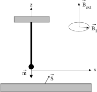
Figure 1: Cantilever set-up. $\vec{B}_{ext}$ is the external static magnetic field, $\vec{B}_{1}$ the rotating magnetic field, $\vec{m}$ the magnetic moment of the ferromagnetic particle glued on the cantilever tip, $\vec{S}$ the spin to be measured.

The dimensionless Hamiltonian for the OSCAR MRFM in the rotating system of coordinates is taken as

$${\cal H}=(p_{x}^{2}+x^{2})/2+\varepsilon S_{x}+2\eta xS_{z},$$ (1)

where we use the quantum units of the momentum $P_{0}=\hbar/X_{0}$ and the coordinate $X_{0}=\sqrt{\hbar\omega_{c}/k_{c}}$. Here $\omega_{c}$ is the cantilever frequency, $k_{c}$ is the cantilever effective spring constant, $\varepsilon=\gamma B_{1}/\omega_{c}$, $\gamma$ is the magnitude of the electron gyromagnetic ratio and $\eta=(1/2)(\gamma X_{0}/\omega_{c})G$, where $G=\partial B_{z}/\partial x$, is the magnetic field gradient at the spin location. The first term in (1) describes the unperturbed oscillations of the CT, the second term describes the interaction between the spin and the resonant rf field, and the last term describes the interaction between the spin and the CT. To take into consideration the magnetic noise on the spin caused by the thermal CT vibrations we add a random term $\Delta(t)S_{z}$ to the Hamiltonian (1).

The wave function of the system is assumed to have the form

$$\Psi=u_{\alpha}(x,\tau){\bf{\alpha}}+u_{\beta}(x,\tau){\bf{\beta}},$$ (2)

where ${\bf{\alpha}}$ and ${\bf{\beta}}$ are the basis spin functions in the $S_{z}$ representation corresponding to the values $S_{z}=\pm 1/2$, and $\tau=\omega_{c}t$ is the dimensionless time. The Schrödinger equation splits into two coupled equations for $u_{\alpha}(x,\tau)$ and $u_{\beta}(x,\tau)$. If these two functions are identical (up to a constant factor) then the wave function can be represented by a product of the CT and spin wave functions. In this case the average spin $\langle{\vec{S}}\rangle$ has a magnitude 1/2. In the general case, the spin is entangled with the CT, and the average spin is smaller than 1/2. In our estimates we will use the following parameters from experiment 1 :

$$\begin{array}[]{lll}&\omega_{c}/2\pi=6.6kHz,~{}k_{c}=600\mu N/m,~{}B_{1}=300\mu T,\\ &G=4.3\times 10^{5}T/m,~{}X_{m}=10nm,~{}T=200mK,\\ \end{array}$$ (3)

where $X_{m}$ is the amplitude of the CT. Using these values, we obtain the following values of parameters for our model

$$\begin{array}[]{lll}X_{0}&=85fm,~{}P_{0}=1.2\times 10^{-21}Ns,~{}\eta=0.078,\\ x_{m}&=X_{m}/X_{0}=1.2\times 10^{5}.\end{array}$$ (4)

The relative frequency shift $\delta\omega_{0}=|\Delta\omega_{c}/\omega_{c}|$ of the cantilever vibrations can be estimated to be 6 ; 7 :

$$\delta\omega_{0}=2S\eta^{2}/(2\eta^{2}x^{2}_{m}+\varepsilon^{2})^{1/2}=4.7\times 10^{-7}.$$ (5)

(We insert the factor $2S$ for future discussion.)

Suppose that initially the spin points opposite to the direction of ${\vec{B}}_{eff}$. The frequency shift of the CT vibrations is then $-\delta\omega_{0}$. The magnetic noise acting on the spin causes a deviation of the spin direction from the direction of the effective magnetic field. Thus, it produces two trajectories of the CT with the frequencies $\pm\delta\omega_{0}$. Because of the quantum uncertainty of the CT position during the finite time (which we call the collapse time $\tau_{coll}$), the wave function of the CT describes a single peak with an absolute value of the frequency shift less than $\delta\omega_{0}$. The collapse of the wave function changes the frequency shift to the value $-\delta\omega_{0}$ (or, sometimes, $\delta\omega_{0}$, in the case of a quantum jump).

We simulate the quantum dynamics between two consecutive collapses of the wave function of the system. In our simplified model the magnetic noise $\Delta(t)$ takes consecutively two values, $\pm\Delta_{0}$. The time interval between two consecutive “kicks” of the function $\Delta(t)$ was taken randomly from the interval $(-3\tau_{R}/4,5\tau_{R}/4)$, where $\tau_{R}=2\pi/\varepsilon$ is the dimensionless Rabi period. (In a more advanced theory the characteristics of the magnetic noise should be derived from the parameters of the thermal CT vibrations.) The initial wave function is assumed to be a direct product of the CT and spin wave functions. The initial state of the CT is a coherent state

$$|\alpha_{0}\rangle=\pi^{1/4}\sum_{n}2^{n/2}\alpha_{0}^{n}H_{n}(x)\exp\{-(x^{2}+|\alpha_{0}|^{2})/2\},$$ (6)

where $H_{n}(x)$ is a Hermite polynomial, and $\alpha_{0}={{1}\over{\sqrt{2}}}(x_{0}+p_{0})$; here $x_{0}$ and $p_{0}$ are the quantum mechanical averages of $x$ and $p$ at $\tau=0$. The initial direction of the spin is taken to be opposite to the direction of the effective magnetic field $\vec{B}_{eff}=\vec{i}\varepsilon+2\vec{k}\eta x_{0}$, where $\vec{i}$ and $\vec{k}$ are the unit vectors in the positive $x$- and $z$-directions.

In our numerical simulations we expand the functions $u_{\alpha}(x,\tau)$ and $u_{\beta}(x,\tau)$ in (2) over 400 eigenfunctions of the unperturbed oscillator Hamiltonian. During the time interval between two consecutive “kicks” of the noise function $\Delta(t)$ we have a time-independent Hamiltonian. Thus, we find the evolution of the wave function by diagonalizing the $800\times 800$ matrix and taking into consideration the initial conditions after each “kick”. The output of our simulations is the time interval $\Delta\tau_{j}=\tau_{j}-\tau_{j-1}$ between two consecutive returns to the origin for the average value $\langle x\rangle$: $\langle x(\tau_{j-1})\rangle=0$ and $\langle x(\tau_{j})\rangle=0$. To save computational time, we have used the values of parameters $\varepsilon=10$, $\eta=0.3$, $p_{0}=0$, $x_{0}=13$. These values provide a relative large frequency shift of the CT oscillations 7 ; 8

$$\delta\omega_{0}\approx 7.9\times 10^{-3}.$$ (7)

The results of our simulations are shown in Fig. 2, which demonstrates the deviation of $\Delta\tau_{j}$ from the unperturbed half-period of the CT oscillations $\pi$. We introduce $\delta\tau_{j}=|\Delta\tau_{j}-\pi|$. With no magnetic noise $(\Delta_{0}=0)$ the deviation $\delta\tau_{j}$ does not change with time

$$\delta\tau_{j}=\delta\tau_{0}=\pi/\delta\omega_{0}\approx 0.025.$$ (8)

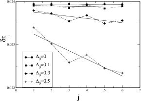
Figure 2: Deviation of $\Delta\tau_{j}$ from the unperturbed half period of the CT oscillations $\pi$, as a function of the number of half periods $j$, for different $\Delta_{0}$ as indicated in the legend. Solid lines are the standard linear fits. On the vertical axis $\delta\tau_{j}=|\Delta\tau_{j}-\pi|$.

If $\Delta_{0}\not=0$, the value of $\delta\tau_{j}$ decreases with time until the collapse of the wave function destroys the Schrödinger cat state. (Fig. 2 demonstrates the case for which the time interval between the collapses equals six half-periods of the CT vibrations).

We will define the “effective frequency” $\omega_{j}$ for each half-period of the CT vibrations: $\omega_{j}=\pi/\Delta\tau_{j}$. Next, we introduce the effective frequency shift $\delta\omega_{j}=\pi/\delta\tau_{j}$. From Fig. 2 we can find the average effective frequency shift $\langle\delta\omega\rangle$ between two collapses of the wave function.

If our model of the noise were the adequate one, then from the experimentally measured quantity $\langle\delta\omega\rangle$ we could determine the time interval between two collapses $\tau_{coll}$. (It is clear from Fig. 2 that $\langle\delta\omega\rangle$ is directly related to the value of $\tau_{coll}$ for the assumed magnetic noise parameters.) Certainly, in a real situation this opportunity does exist if the average frequency shift $\langle\delta\omega\rangle$ is significantly smaller than the expected shift $\delta\omega_{0}$. We will call such situation “the case of the strong noise”.

Note, that a decrease of the frequency shift may be interpreted as an effective decrease of the spin $\delta S$. Using Eq.(5) we obtain

$$\delta S=(\langle\delta\omega\rangle-\delta\omega_{0})(2\eta^{2}x_{m}^{2}+\varepsilon^{2})^{1/2}/(2\eta^{2}).$$ (9)

Previously we have shown that in the case of strong noise, an experimentalist could determine the time interval $\tau_{coll}$ between two consecutive collapses of the wave function by measuring the decrease of the frequency shift of the CT vibrations. Here we propose a special experiment which allows one to determine the time $\tau_{coll}$ for the case of weak noise in which the average frequency shift between two collapses is close to $\delta\omega_{0}$.

The problem is the following. Even a very weak noise generates a second CT trajectory with a frequency shift opposite to that of the first trajectory. Thus, two trajectories tend to separate at the same rate for any magnetic noise. Correspondingly, the time interval between two collapses is expected to be approximately the same for any level of magnetic noise. However, in the case of weak noise, the probability of the second trajectory is small, so its contribution to the average frequency shift becomes negligible.

To overcome this obstacle, we propose an artificial change of the frequency shift using the “interrupted OSCAR technique” recently implemented in 1 . In 1 , the rf field is turned off for a time interval equal to half of the CT period, which is equivalent to the application of the $\pi$-pulse which changes the direction of the spin relative to the effective magnetic field. We propose to turn off the rf field for the duration of the quarter of the CT period, which is equivalent to the application of the $\pi/2$-pulse. Suppose that initially the spin is parallel to the effective magnetic field, ${\vec{B}}_{eff}$. If we apply a “$\pi/2$-pulse”, the spin will become perpendicular to ${\vec{B}}_{eff}$. Thus, we have two CT trajectories, each with the same probability. Before these two trajectories are separated, the CT will oscillate with the unperturbed frequency, which is equal to one in our dimensionless units. After the collapse the frequency shift is $\pm\delta\omega_{0}$, with equal probabilities. Thus, using a “$\pi/2$-pulse” we can achieve a maximum possible reduction of the frequency shift. If we apply a periodic sequence of “$\pi/2$-pulses” with the period $\tau_{p}$ ($\tau_{p}>\tau_{coll}$), then the average frequency shift $\langle\delta\omega\rangle$ is

$$\langle\delta\omega\rangle=\delta\omega_{0}(\tau_{p}-\tau_{coll})/\tau_{p}.$$ (10)

Manipulating $\tau_{p}$ one can achieve a significant decrease of $\langle\delta\omega\rangle$ in comparison with $\delta\omega_{0}$. Using Eq. (10) one can determine the collapse time from the experimental value $\langle\delta\omega\rangle$. Thus, the collapse time can be measured for the case of weak magnetic noise. Finally, based on quasiclassical theory 5 we will estimate the reduction of the average frequency shift caused by the noise for the experimental conditions 1 . The amplitude of the thermal CT vibrations near the Rabi frequency can be estimated to be:

$$a_{T}=(\omega_{c}/\omega_{R})(k_{B}T/2k_{c})^{1/2}=38fm.$$ (11)

The square of the characteristic spin deviation during a single reversal (half of the CT period) is

$$(\Delta\theta_{1})^{2}\approx 3.4Ga^{2}_{T}/(\omega_{c}X_{m})=9\times 10^{-7}.$$ (12)

We have no idea about the order of the collapse time $\tau_{coll}$. If we assume that the collapse occurs when the separation between the two trajectories with the frequencies $1\pm\delta\omega_{0}$ is equal to $1/2$ (the quantum uncertainty of the CT position in the coherent state is $\langle(\Delta x)^{2}\rangle=1/2$), then we obtain for $\tau_{coll}$

$$\tau_{coll}\sin\tau_{coll}\approx 1/(4x_{m}\delta\omega_{0})\approx 4.4.$$ (13)

It follows from Eq.(13) that the wave function collapses during the second period of the CT vibrations. If we estimate the probabilities of the two CT trajectories as $P_{1}\sim 1-(\Delta\theta_{1})^{2}$ (for the trajectory with the initial frequency shift) and $P_{2}\sim(\Delta\theta_{1})^{2}$ (for the trajectory with the opposite frequency shift), then the average CT frequency shift can be estimated to be

$$\langle\delta\omega\rangle=\delta\omega_{0}(P_{1}-P_{2})=\delta\omega_{0}(1-2(\Delta\theta_{1})^{2}).$$ (14)

This estimated reduction of the CT frequency shift is clearly negligible.

Consider the opposite extreme case. Suppose that the collapse occurs when the separation between the two trajectories is of the order of the thermal CT fluctuations $(k_{B}T/k_{c})^{1/2}\approx 150$pm or $1760$ in dimensionless units (as before, we used the values of parameters in (3)). In this case, the time interval between the two consecutive collapses $\tau_{coll}$ is of the order of $10^{4}$ periods of the CT oscillations. During this time, the characteristic spin deviation is $(\Delta\theta)^{2}\sim 0.02$. Then, we have for the probability $P_{1}\approx(\Delta\theta)^{2}/4\approx 5\times 10^{-3}$. The average frequency shift is $\langle\delta\omega\rangle\approx\delta\omega_{0}(1-10^{-2})$. One can see that even in this extreme case the reduction of the frequency shift is expected to be small.

Thus, the experimental conditions in 1 probably correspond to the case of the weak noise. In such a situation the collapse time could be measured using the periodic sequence of “$\pi/2$-pulses” described earlier.

We have demonstrated a procedure for measuring the mysterious collapse time in the OSCAR MRFM technique. We simulated the quantum dynamics of the spin-CT system. Unlike the previous studies of the quantum dynamics we took into consideration the direct interaction between the spin and the environment (the magnetic noise). This noise causes (i) a deviation of the spin from the direction of the effective magnetic field and (ii) entanglement between the spin and the CT. For the case of weak magnetic noise, the same effect can be achieved the effective “$\pi/2$-pulses” with the “interrupted OSCAR” technique. The spin-CT entanglement influences the frequency of the CT oscillations before the wave function collapse takes place. This effect can be described as an effective decrease of the single spin magnitude. We demonstrated that the experimental measurement of the OSCAR MRFM frequency shift could reveal information about the time interval between two consecutive collapses of the wave function.

We thank D. Rugar and G.D. Doolen for discussions. This work was supported by the Department of Energy (DOE) under Contract No. W-7405-ENG-36, by the Defense Advanced Research Projects Agency (DARPA), by the National Security Agency (NSA), and by the Advanced Research and Development Activity (ARDA).

References

- (1) H.J. Mamin, R. Budakian, B.W. Chui, D. Rugar, Phys. Rev. Lett., 91, 207604 (2003).
- (2) B.C. Stipe, H.J. Mamin, C.S. Yannoni, T.D. Stowe, T.W. Kenny, D. Rugar, Phys. Rev. Lett., 87 277602 (2001).
- (3) G.P. Berman, D.I. Kamenev, V.I. Tsifrinovich, Phys. Rev. A, 66, 023405 (2002).
- (4) G.P. Berman, V.N. Gorshkov, D. Rugar, V.I. Tsifrinovich, Phys. Rev. B, 68, 094402 (2003).
- (5) G.P. Berman, V.N. Gorshkov, V.I. Tsifrinovich, Phys. Lett. A, 318, 584 (2003).
- (6) D. Mozyrsky, I. Martin, D. Pelekhov, P.C. Hammel, Appl. Phys. Lett., 82, 1278 (2003).
- (7) G.P. Berman, F. Borgonovi, V.I. Tsifrinovich, Quantum Information and Computation, 4, 102 (2004).
- (8) G.P. Berman, F. Borgonovi, Z. Rinkevicius, V.I. Tsifrinovich. Superlattices and Microstructures, to be published (2004).
- (9) G.P. Berman, F. Borgonovi, V.I. Tsifrinovich, quant-ph/0402063.
- (10) W.H. Zurek, Physics Today, 44, 36 (1991).
- (11) G.P. Berman, F. Borgonovi, G.V. Lopez, V.I. Tsifrinovich, Phys. Rev. A., 68, 012102 (2003).