Entanglement of distant electron interference experiments

Abstract

Two electron interference experiments which are far from each other, are considered. They are irradiated with correlated nonclassical electromagnetic fields, produced by the same source. The phase factors are in this case operators, and their expectation values with respect to the density matrix of the electromagnetic field quantify the observed electron fringes. The correlated photons create correlations between the observed electron intensities. Both cases of classically correlated (separable) and quantum mechanically correlated (entangled) electromagnetic fields are considered. It is shown that the induced correlation between the distant electron interferences is sensitive to the nature of the correlation between the irradiating photons.

Phys. Rev. A 69, 013810 (2004).

I Introduction

Interference of electrons encircling a magnetostatic flux has been studied extensively since the work of Aharonov and Bohm AB ; SM . These ideas have been applied in various contexts, for example, in magnetoconductance oscillations in mesoscopic rings SS , “which-path” experiments WP , and neutron interferometry NI .

The Aharonov-Bohm effect can be generalized by replacing the magnetostatic flux with an electromagnetic field. The objective in this “ac Aharonov-Bohm” effect is very different from the “dc Aharonov-Bohm” effect (with magnetostatic flux). In the latter case the physical reality of the vector potential has been demonstrated and the subtleties of quantum mechanics in nontrivial topologies have been studied. The former case constitutes a nonlinear device, where the interaction between the interfering electrons and the photons leads to interesting nonlinear phenomena. Indeed the nonlinearity can be seen in the intensity of the interfering electrons which is a sinusoidal function of the time-dependent magnetic flux. In Refs. 1 ; 2 the interference of electric charges in the presence of both classical and nonclassical electromagnetic fields, has been studied. It has been shown that the quantum noise of the electromagnetic field affects the phase factor.

In this paper we consider two Aharonov-Bohm interference devices which are far from each other. Each of them is irradiated with a nonclassical electromagnetic field. The aim of the paper is to consider entanglement between the two electromagnetic modes irradiating the two Aharonov-Bohm interference devices and study the correlations between the interfering electrons in the two devices. We note that in Refs. 2 we have studied the effect of photon entanglement on a single Aharonov-Bohm interference device. Here we consider two electron interference devices far apart from each other, and show that the two electron interferences are correlated due to the entanglement between the two electromagnetic fields.

In Sec. II we describe the experiment. We show that the joint electron intensity depends on the density operator describing the two-mode electromagnetic field. In Sec. III we consider two cases for the density operator of the field, separable and entangled EN . We conclude in Sec. IV with a discussion of the results.

II Electron interference

We consider two electron interference experiments far apart from each other, which we refer to as A and B (Fig. 1). They are irradiated with electromagnetic fields. Each electron beam splits into two paths $C_{A0},C_{A1}$ and $C_{B0},C_{B1}$ (paths with higher winding numbers are ignored).

Let $\phi_{A}$ be the time dependent flux threading the loop $C_{A1}-C_{A0}$. The electron wave function at the point $x_{A}$ is given by 1 ; 2

$$\Psi_{A}(x_{A})=\psi_{A0}(x_{A})+\exp(ie\phi_{A})\psi_{A1}(x_{A}),$$ (1)

where $\psi_{A0}(x_{A})$ and $\psi_{A1}(x_{A})$ are the electron wave functions associated with the paths $C_{A0}$ and $C_{A1}$, correspondingly. This leads to the electron intensity

$$I_{A}(\sigma_{A}) = 1+\cos(\sigma_{A}+e\phi_{A}),$$ (2)

$$\sigma_{A} \equiv \arg[\psi_{A1}(x_{A})]-\arg[\psi_{A0}(x_{A})],$$

for the case of equal splitting between the two wave functions ($|\psi_{A0}(x_{A})|^{2}=1/2=|\psi_{A1}(x_{A})|^{2}$). We note that the phase difference $\sigma_{A}$ is effectively a rescaled position $x_{A}$ on the screen. All the results below are in terms of $\sigma_{A}$ (and $\sigma_{B}$).

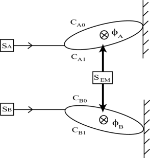
Figure 1: Two electron interference experiments which are far from each other are irradiated with nonclassical electromagnetic fields. The two electromagnetic fields in the two experiments are produced by the source $S_{EM}$ and are correlated.

II.1 Nonclassical electromagnetic fields

As explained in our previous work 1 ; 2 for a nonclassical electromagnetic field of frequency $\omega$ the flux $\phi$ is an operator. The dual quantum variables of the electromagnetic field are the vector potential $A_{i}$ and the electric field $E_{i}$. Although the dual quantum variables are local quantities, we consider loops which are small in comparison to the wavelength and after integration we get $\hat{\phi}=\oint_{C}A_{i}dx_{i}$ and the electromotive force $\hat{V}=\oint_{C}E_{i}dx_{i}$ as dual quantum variables. We next introduce the corresponding creation and annihilation operators, $\hat{a}^{{\dagger}}=2^{-1/2}\xi^{-1}(\hat{\phi}-i\omega^{-1}\hat{V})$ and $\hat{a}=2^{-1/2}\xi^{-1}(\hat{\phi}+i\omega^{-1}\hat{V})$, where $\xi$ is a constant proportional to the area enclosed by the loop and in units $k_{B}=\hbar=c=1$. We work in the “external field approximation” where the back-reaction from the electrons on the electromagnetic field is neglected. This is valid for external fields which are strong in comparison to those produced dynamically by the electrons (back-reaction). In this case we get $\hat{\phi}(t)=2^{-1/2}\xi[\exp(i\omega t)\hat{a}^{\dagger}+\exp(-i\omega t)\hat{a}]$.

Exponentiation of the magnetic flux operator yields the phase factor $\exp[ie\hat{\phi}(t)]$, which becomes

$$\exp[ie\hat{\phi}(t)]=D[iq\exp(i\omega t)];\;\;\;q=2^{-1/2}\xi e,$$ (3)

where $D(x)=\exp(x\hat{a}^{{\dagger}}-x^{*}\hat{a})$ is the displacement operator. In order to find expectation values we take the trace of the $\exp[ie\hat{\phi}(t)]$ operator with respect to the density matrix $\rho$ describing the nonclassical electromagnetic field:

$${\rm Tr}\{\rho\exp[ie\hat{\phi}(t)]\} = \mbox{Tr}[\rho D(\lambda)]\equiv\tilde{W}(\lambda)$$

$$\lambda = iq\exp(i\omega t).$$ (4)

Here $\tilde{W}$ is the Weyl or characteristic or ambiguity function (cf. Ref. WW and references therein). The tilde in the notation reflects the fact that the Weyl function is the two-dimensional Fourier transform of the Wigner function (which is usually denoted by $W$).

II.2 Correlated electron intensities

Let $\rho$ be the density operator describing the two-mode nonclassical electromagnetic field in both devices. The first mode of frequency $\omega_{1}$ interacts with electrons in experiment ${\rm A}$ and its density matrix is $\rho_{A}\equiv{\rm Tr}_{B}\rho$. The second mode of frequency $\omega_{2}$ interacts with electrons in experiment ${\rm B}$ and its density matrix is $\rho_{B}\equiv{\rm Tr}_{A}\rho$.

For nonclassical electromagnetic fields the flux and consequently the intensity of Eq. (2) are operators. In order to find the expectation value of the intensity we calculate its trace with respect to the appropriate density matrix and using Eq. (II.1) we find

$$I_{A}(\sigma_{A}) = \mbox{Tr}\{\rho_{A}[1+\cos(\sigma_{A}+e\hat{\phi}_{A})]\}$$ (5)

$$= 1+|\tilde{W}(\lambda_{A})|\cos\{\sigma_{A}+\arg[\tilde{W}(\lambda_{A})]\}.$$

where $\lambda_{A}=iq\exp(i\omega_{1}t)$. As we have explained in detail in our previous work 1 ; 2 , the visibility in this case is $|\tilde{W}(\lambda_{A})|$ which takes values less than $1$. It has been shown there that this is intimately related to the quantum uncertainties in the electric and magnetic fields and consequently the reduction of the visibility from $1$ to $|\tilde{W}(\lambda_{A})|$ is due to the quantum noise in the nonclassical fields.

Similarly the electron intensity in experiment ${\rm B}$ is

$$I_{B}(\sigma_{B}) = \mbox{Tr}\{\rho_{B}[1+\cos(\sigma_{B}+e\hat{\phi}_{B})]\}$$ (6)

$$= 1+|\tilde{W}(\lambda_{B})|\cos\{\sigma_{B}+\arg[\tilde{W}(\lambda_{B})]\},$$

where $\lambda_{B}=iq\exp(i\omega_{2}t)$.

We next consider the joint electron intensity in the two experiments. It is given by

$$I(\sigma_{A},\sigma_{B})=$$ (7)

$$\mbox{Tr}\{\rho[1+\cos(\sigma_{A}+e\hat{\phi}_{A})][1+\cos(\sigma_{B}+e\hat{\phi}_{B})]\}.$$

The correlations between the electron interferences in the two experiments are quantified with the ratio

$$R=\frac{I(\sigma_{A},\sigma_{B})}{I_{A}(\sigma_{A})I_{B}(\sigma_{B})}.$$ (8)

III Examples

Two mode density matrices are factorizable (uncorrelated) if they can be written as $\rho=\rho_{A}\otimes\rho_{B}$. They are separable (classically correlated) if they can be written as $\rho=\sum_{i}p_{i}\rho_{A,i}\otimes\rho_{B,i}$ where $p_{i}$ are probabilities. Density matrices which cannot be written in one of these two forms are entangled (quantum mechanically correlated). There has been a lot of work on criteria which distinguish separable and entangled states EN . In this paper we compare and contrast the influence of separable and entangled photon states on two distant electron interference experiments.

We consider two cases for the density operator $\rho$ of the two-mode electromagnetic fields. The first is the separable (classically correlated) density matrix

$$\rho_{{\rm sep}}=\frac{1}{2}(|01\rangle\langle 01|+|10\rangle\langle 10|).$$ (9)

The second is the entangled state $|\mbox{S}\rangle=2^{-1/2}(|01\rangle+|10\rangle)$ with corresponding density matrix

$$\rho_{{\rm ent}} = \rho_{{\rm sep}}+\frac{1}{2}(|01\rangle\langle 10|+|10\rangle\langle 01|),$$ (10)

where $\rho_{\rm sep}$ is given by Eq. (9). The difference between $\rho_{\rm sep}$ and $\rho_{\rm ent}$ lies in the above non-diagonal elements.

III.1 Classically correlated number eigenstates

In the case of separable electromagnetic fields of Eq. (9) the electron intensities are

$$I_{A}(\sigma_{A}) = 1+\alpha\cos\sigma_{A},$$ (11)

$$I_{B}(\sigma_{B}) = 1+\alpha\cos\sigma_{B},$$

where

$$\alpha=\frac{2-q^{2}}{2}\exp\left(-\frac{q^{2}}{2}\right).$$ (12)

As explained in detail in Refs. 1 ; 2 the visibility corresponding to $I_{A}$ or $I_{B}$ is $\alpha<1$, due to the noise in the nonclassical electromagnetic fields.

We also calculate the joint intensity

$$I_{\rm sep}(\sigma_{A},\sigma_{B}) = 1+\alpha(\cos\sigma_{A}+\cos\sigma_{B})$$ (13)

$$+2\beta\cos\sigma_{A}\cos\sigma_{B},$$

where

$$\beta=\frac{1-q^{2}}{2}\exp\left(-q^{2}\right).$$ (14)

The ratio $R$ of Eq. (8) is

$$R_{\rm sep}(\sigma_{A},\sigma_{B})=$$ (15)

$$\frac{1+\alpha(\cos\sigma_{A}+\cos\sigma_{B})+2\beta\cos\sigma_{A}\cos\sigma_{B}}{(1+\alpha\cos\sigma_{A})(1+\alpha\cos\sigma_{B})}.$$

$R_{\rm sep}(\sigma_{A},\sigma_{B})$ is periodic in $\sigma_{A}$ and $\sigma_{B}$ with period $2\pi$ for each of the screen positions. Its stationary points are such that $\frac{\partial R_{\rm sep}}{\partial\sigma_{A}}=0=\frac{\partial R_{\rm sep}}{\partial\sigma_{B}}$ and it can easily be shown that

$$\frac{1-2\alpha+2\beta}{(1-\alpha)^{2}}\leq R_{\rm sep}(\sigma_{A},\sigma_{B})\leq\frac{1+2\alpha+2\beta}{(1+\alpha)^{2}}.$$ (16)

The global minimum occurs at the point $(\sigma_{A}=\pi,\sigma_{B}=\pi)$ and the global maxima at the points $(\sigma_{A}=0~{}\mbox{or}~{}2\pi,\sigma_{B}=0~{}\mbox{or}~{}2\pi)$.

We note that for factorizable (uncorrelated) electromagnetic fields $R=1$. In the example of separable (classically correlated) electromagnetic fields of Eq. (9) we get $R_{\rm sep}$ independent of time, which takes values less than $1$ (the upper bound in the inequality (16) is slightly less than $1$).

III.2 Entangled number eigenstates

We now consider the entangled electromagnetic fields of Eq. (10). In this case the electron intensities $I_{A}(\sigma_{A})$ and $I_{B}(\sigma_{B})$ are the same as in Eq. (11). The joint electron intensity is

$$I_{\rm ent}(\sigma_{A},\sigma_{B})=I_{\rm sep}(\sigma_{A},\sigma_{B})$$ (17)

$$- q^{2}\exp(-q^{2})\sin\sigma_{A}\sin\sigma_{B}\cos[(\omega_{1}-\omega_{2})t],$$

and the ratio of Eq. (8) is

$$R_{\rm ent}(\sigma_{A},\sigma_{B}) = R_{\rm sep}(\sigma_{A},\sigma_{B})-q^{2}\exp(-q^{2})$$ (18)

$$\times\frac{\sin\sigma_{A}\sin\sigma_{B}\cos[(\omega_{1}-\omega_{2})t]}{(1+\alpha\cos\sigma_{A})(1+\alpha\cos\sigma_{B})}.$$

It is seen that $I_{\rm ent}(\sigma_{A},\sigma_{B})$ is equal to $I_{\rm sep}(\sigma_{A},\sigma_{B})$ of Eq. (13) plus an extra term, which oscillates in time with frequency $\omega_{1}-\omega_{2}$ around this value. In the case $\omega_{1}=\omega_{2}$ the electron intensity $I_{\rm ent}(\sigma_{A},\sigma_{B})$ differs from the electron intensity $I_{\rm sep}(\sigma_{A},\sigma_{B})$ by a constant (which depends on $\sigma_{A}$, $\sigma_{B}$). Similar comments apply to $R_{\rm sep}(\sigma_{A},\sigma_{B})$ and $R_{\rm ent}(\sigma_{A},\sigma_{B})$

III.3 Numerical results

In all numerical results the electromagnetic fields have frequencies $\omega_{1}=1.2\times 10^{-4}$ and $\omega_{2}=10^{-4}$, and the parameter $\xi=1$. Fig. 2 shows the $I_{\rm sep}(\sigma_{A},\sigma_{B})$ of Eq. (13) as a function of $\sigma_{A}$ and $\sigma_{B}$. Fig. 3 shows the $R_{\rm sep}(\sigma_{A},\sigma_{B})$ of Eq. (15). We note that in our example the $R_{\rm sep}$ is time-independent and $\min(R_{\rm sep})=0.7557$, $\max(R_{\rm sep})=0.995$.

Fig. 4 shows $R_{\rm ent}$ at $(\omega_{1}-\omega_{2})t=\pi$ as a function of $\sigma_{A}$ and $\sigma_{B}$. Fig. 5 is a slice of Fig. 4 for $\sigma_{B}=-1.1\pi$. Fig. 6 shows the time variation of the two ratios, $R_{\rm sep}$ (line of circles) and $R_{\rm ent}$ (continuous line), for $\sigma_{A}=0.98\pi$ and $\sigma_{B}=-1.1\pi$.

The results show that both classically and quantum mechanically correlated photons induce correlations on the distant electron interference experiments. We have compared and contrasted two examples: the $\rho_{\rm sep}$ of Eq. (9), which is a mixed state; and the $\rho_{\rm ent}$ of Eq. (10), which is a maximally entangled pure state. These two density matrices of the electromagnetic field differ only by off-diagonal elements. We have shown that the effect of these off-diagonal elements on the correlations between the electron interference experiments, is drastic (compare and contrast Figs. 3 and 4).

IV Discussion

We have considered electron interference experiments irradiated with nonclassical electromagnetic fields. In this case the phase factor is the quantum mechanical operator of Eq.(3) and its expectation value with respect to the density matrix of the electromagnetic field, affects the interference. In this general context, we have studied the case of two electron interference experiments that are far from each other and are irradiated with two electromagnetic fields of frequencies $\omega_{1},\omega_{2}$. The two electromagnetic fields are produced by the same source and are correlated; consequently the expectation values of the two phase factor operators in the two experiments are also correlated.

The examples of Eqs. (9) and (10) have been considered. They represent classically correlated (separable) and quantum mechanically correlated (entangled) electromagnetic fields, correspondingly. Due to the correlations in the electromagnetic field the electron fringes are also correlated. This has been quantified with the ratio $R$ of Eq. (8). In the example considered the $R_{\rm sep}$ (Eq. (15)) is time-independent and takes values less than $1$. The $R_{\rm ent}$ (Eq. (18)) oscillates sinusoidally in time (with frequency $\omega_{1}-\omega_{2}$) around the value $R_{\rm sep}$. In the case $\omega_{1}=\omega_{2}$ the ratio $R_{\rm ent}(\sigma_{A},\sigma_{B})$ differs from $R_{\rm sep}(\sigma_{A},\sigma_{B})$ by a constant (which depends on $\sigma_{A}$, $\sigma_{B}$).

Other examples, can also be calculated. But the examples considered show clearly the main point of the paper, which is that distant electron interference experiments can be correlated through correlated photons. We have also shown that the correlations of these distant electron interference fringes are sensitive to the off-diagonal elements of the electromagnetic density matrix.

The work brings together concepts from generalized Aharonov-Bohm phenomena irradiated with nonclassical electromagnetic fields and concepts from nonclassical correlations and entanglement. The results demonstrate that entangled electromagnetic fields interacting with electrons produce entangled electrons.

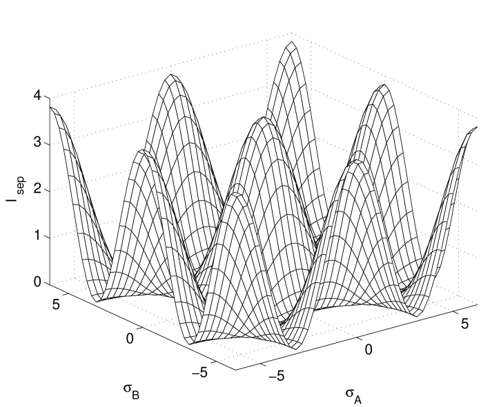
Figure 2: $I_{\rm sep}$ as a function of $\sigma_{A},\sigma_{B}\in[-2\pi,2\pi]$. The frequencies are $\omega_{1}=1.2\times 10^{-4}$ and $\omega_{2}=10^{-4}$, in units where $k_{B}=\hbar=c=1$.

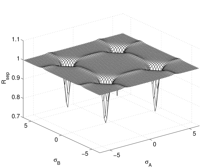
Figure 3: $R_{\rm sep}$ as a function of $\sigma_{A},\sigma_{B}\in[-2\pi,2\pi]$. Here $\min(R_{\rm sep})=0.7557$ and $\max(R_{\rm sep})=0.995$. The frequencies are $\omega_{1}=1.2\times 10^{-4}$ and $\omega_{2}=10^{-4}$, in units where $k_{B}=\hbar=c=1$.

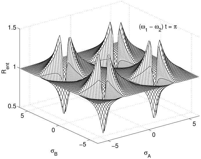
Figure 4: $R_{\rm ent}$ as a function of $\sigma_{A},\sigma_{B}\in[-2\pi,2\pi]$, at $t=(\omega_{1}-\omega_{2})^{-1}\pi$. The frequencies are $\omega_{1}=1.2\times 10^{-4}$ and $\omega_{2}=10^{-4}$, in units where $k_{B}=\hbar=c=1$.

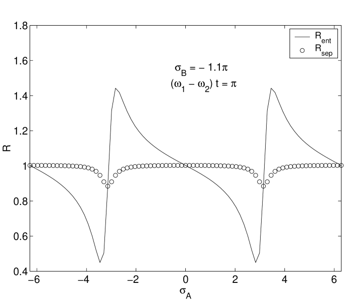
Figure 5: Comparison of $R_{\rm ent}$ (continuous line) and $R_{\rm sep}$ (line of circles) against $\sigma_{A}$ for $(\omega_{1}-\omega_{2})t=\pi$ and $\sigma_{B}=-1.1\pi$. Note that $\max(R_{\rm sep})=0.995$. The frequencies are $\omega_{1}=1.2\times 10^{-4}$ and $\omega_{2}=10^{-4}$, in units where $k_{B}=\hbar=c=1$.

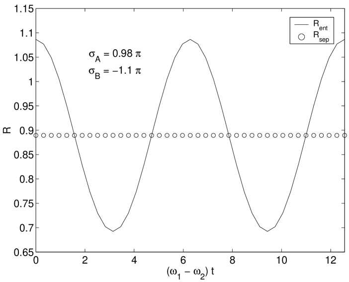
Figure 6: Comparison of $R_{\rm ent}$ (continuous line) and $R_{\rm sep}$ (line of circles) for $\sigma_{A}=0.98\pi$ and $\sigma_{B}=-1.1\pi$ as a function of dimensionless time. The frequencies are $\omega_{1}=1.2\times 10^{-4}$ and $\omega_{2}=10^{-4}$. We use units where $k_{B}=\hbar=c=1$.

References

(1) Y. Aharonov and D. Bohm, Phys. Rev. 115, 485 (1959);
M. Peshkin and A. Tonomura, The Aharonov-Bohm effect, Lecture notes in Physics, Vol. 340
(Springer, Berlin, 1989).
(2) M.P. Silverman, More than one mystery: explorations in quantum interference
(Springer, New York, 1994).
(3) S. Washburn and R.A. Webb, Adv. Phys.35, 375 (1986);
A.G. Aronov and Y.V. Sharvin, Rev. Mod. Phys.59, 755
(1987); M. Pepper, Proc. R. Soc. Lond. A 420, 1 (1988).
(4) A. Yacoby, M. Heiblum, D. Mahalu, and H. Shtrikman, Phys. Rev. Lett.74, 4047
(1995); E. Buks et. al., Nature391, 871
(1998); G. Hackenbroich, Phys. Rep.343, 464 (2001).
(5) G. Badurek, H. Rauch, and J. Summhammer, Phys. Rev. Lett.51, 1015
(1983);
J. Summhammer, Phys. Rev. A 47, 556 (1993);
J. Summhammer et al., Phys. Rev. Lett.75, 3206 (1995).
(6) A. Vourdas, Europhys. Lett.32, 289 (1995); Phys. Rev. B 54,
13175 (1996).
(7) A. Vourdas, Phys. Rev. A64, 53814 (2001);
C.C. Chong, D.I. Tsomokos, and A. Vourdas, Phys. Rev. A 66,
33813 (2002).
(8) R.F. Werner, Phys. Rev. A 40, 4277 (1989);
A. Peres, Phys. Rev. Lett.77, 1413 (1996);
R. Horodecki and M. Horodecki, Phys. Rev. A 54, 1838 (1996);
V. Vedral et. al., Phys. Rev. Lett.78, 2275 (1997).
(9) S. Chountasis and A. Vourdas, Phys. Rev. A 58, 848 (1998).