Operational formulation of homodyne detection

Abstract

We obtain the standard quadrature-phase positive operator-valued measure (POVM) for homodyne detection directly and rigorously from the POVM for photon counting without directly employing the mean field approximation for the local oscillator. In addition we obtain correction terms for the quadrature-phase POVM that are applicable for relatively weak local oscillator field strengths and typical signal states.

I Introduction

With the advent of squeezed states of light Rad87 , a full quantum description of optical homodyne detection Rad87 ; Yue78 ; Yue79 ; Yue83 assumed importance as homodyne detection (HD) yields phase–dependent measurements of the light field. Whereas photodetectors acquire phase–insensitive information about photon statistics Gla63 ; Sud63 , homodyne detection mixes the signal field with a coherent local oscillator (LO) to yield photon statistics on the output fields that depend on the phase $\varphi$ of the LO. By varying this phase $\varphi$, phase–dependent properties of the signal state $\hat{\rho}$ can be inferred. The phase–sensitive measurement with respect to the in–phase quadrature $x$ or its canonically conjugate out–of–phase quadrature $p$, or some in–between quadrature $x_{\varphi}\equiv p_{\varphi-\pi/2}\equiv x\cos\varphi+p\sin\varphi$, is necessary to observe the nonclassical properties of squeezed light. Phase–sensitive measurement has developed beyond measuring specific quadrature–phase statistics to acquiring information for many values of $\varphi$ and reconstructing the density matrix $\hat{\rho}$ for the signal field. This technique, known as optical homodyne tomography Ris , illustrates another important application of homodyne detection. Homodyne detection has evolved into a key tool of quantum optics with applications including squeezed light detection, optical homodyne tomography and continuous variable quantum teleportation Vai94 ; Bra98 ; Fur98 .

The homodyne detection scheme discussed above involves mixing the signal field with a LO field at a beamsplitter (BS), and the two output fields are subjected to photodetection, as shown in Fig. 1. The measured photodetection statistics are analyzed to infer the quadrature–phase statistics. Only in the limit of infinite LO field strengths can the measurement be said to correspond to quadrature–phase measurements, and, of course, this limit is in principle unattainable. However, a good approximation to quadrature–phase measurements is attained. In the most useful variant, a 50/50 BS is used, and the difference between the photocounts at the two output ports is used to infer the quadrature–phase statistics. This is known as balanced homodyne detection (BHD) and has the advantage of automatically canceling the photon number sum at the two input ports from the detected output fields.

The description of homodyne detection begins with photodetection of the output fields and then, to validate the approximations normally applied in homodyne detection of quadrature–phase POVM, must show that the resultant two–mode photon statistic reduces in some way to the quadrature–phase distribution, for the signal field $\hat{\rho}$. This connection between photon statistics to quadrature–phase, or joint quadrature–phase, measurements has been established via calculations involving quasi-probability distributions or characteristic functions (moment-generating functions) for the electromagnetic field and allowing the local oscillator strength to become infinitely large. Yuen and Shapiro introduced the characteristic function approach in their seminal quantum theory of HD Yue78 , and Walker employs Wigner functions in his analysis of HD Wal87 . Braunstein Bra90 uses the positive $P$-representation in the description of the photon counting statistics, and he emphasizes the quantum nature of the LO as he investigates “the effects of a finite–amplitude fully-quantum-mechanical local oscillator”. Banaszek and Wódkiewicz Ban97 calculate moments of operationally defined quadrature operators, with an emphasis on finite photodetection efficiency, but in contrast to our approach, employ the mean field approximation to the LO from the outset.

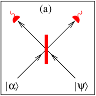
Figure 1: Balanced homodyne detection scheme: (a) the input state $|\psi\rangle$ is mixed with a LO in coherent state $|\alpha\rangle$, and photon counting occurs at the two output ports; (b) photon numbers $j\pm m^{\prime}$ are shown entering the two input ports and $j\pm m$ are counted at the output.

These studies undoubtedly establish the connection between the exact photodetection statistics and the approximate quadrature–phase HD. However, modern applications of homodyne detection, for example to quantum information applications such as continuous–variable quantum teleportation, requires an operational quantum theoretic approach Rud01 ; Banaszek and Wódkiewicz advocate the operational approach, but here we avoid the mean field approximation and thereby include correction terms for the POVM corresponding to HD. The operational approach is important in the context that a measurement may be applied for some purpose other than characterizing the state $\hat{\rho}$; paradoxically, in continuous–variable quantum teleportation Bra98 ; Fur98 , the sender mixes the field described by density operator $\hat{\rho}$ with one component of a two–mode squeezed vacuum state Sch85 in such a way that the sender cannot know, even in principle, what the density operator $\hat{\rho}$ was that is being subjected to this measurement. For such applications, a rigorous approach to homodyne measurement, which demonstrates that the POVM for photodetection reduces to the POVM for quadrature–phase or joint quadrature–phase measurements is necessary. Here we establish this connection between actual and convenient POVMs by directly calculating the photon counting probabilities using two different approaches: (i) working in the Fock basis for the Hilbert space of the signal and LO modes, we employ asymptotic expressions for SU(2) Wigner functions that are the BS matrix elements in the Fock basis; (ii) working in the over-complete basis of coherent states and taking advantage of the simple transformation of coherent states at the BS, we employ the Glauber-Sudarshan $P$-function.

II Balanced homodyne detection scheme

A balanced homodyne detection scheme is depicted in Fig. 1(a). The (generally mixed) signal state $\hat{\rho}$ to be measured is coherently mixed at the BS with a LO assumed to be in a coherent state (in the optical domain a coherent state with an absolute adjustable phase has not been achieved, but the coherent state approach leads to correct measured results provided that the signal field and LO field are derived from the same source Mol97 ; Rud01 ). The photon number difference from the two BS output ports is measured. The photon number sum can also be measured but usually is not. However, in our analysis we include the treatment of both the difference and the sum as this is a more complete description than considering the difference alone. We will denote the photon number difference by $2m\in{\mathbb{Z}}$ and the sum by $2j\in{\mathbb{Z}}$.

The Hilbert space of two modes of electromagnetic field has the basis $\{|n_{1}\rangle\otimes|n_{2}\rangle\}$ of joint eigenstates of the photon number operators $\hat{n}_{1}=\hat{a}_{1}^{\dagger}\hat{a}_{1}$ and $\hat{n}_{2}=\hat{a}_{2}^{\dagger}\hat{a}_{2}$. Denoting $j=(n_{1}+n_{2})/2$, $m=(n_{1}-n_{2})/2$, we will use the notation $|jm\rangle\equiv|n_{1}\rangle\otimes|n_{2}\rangle$. Thus, the state $|jm\rangle$ is the number states with photon numbers $j\pm m$ at modes 1 and 2, respectively. The value of $j$ can be any non-negative half-integer and $m$ can get values $-j,-j+1,\dots,j$ for a given $j$.

II.1 Beam splitter transformation

The beam splitter action on a two-mode state of electromagnetic field is given by the SU(2) transformation Yur86 ; Cam89 ; San95

$$\hat{B}(\varphi_{1},\varphi_{2},\varphi_{3})={\rm e}^{-i\varphi_{1}\hat{J}_{z}}{\rm e}^{-i\varphi_{2}\hat{J}_{y}}{\rm e}^{-i\varphi_{3}\hat{J}_{z}},$$ (1)

where the SU(2) generators $\hat{J}_{y},\hat{J}_{z}$ are expressed in the Schwinger boson representation as

$$\hat{J}_{y}=-\frac{\rm i}{2}(\hat{a}_{1}^{\dagger}\hat{a}_{2}-\hat{a}_{2}^{\dagger}\hat{a}_{1}),\quad\hat{J}_{z}=\frac{1}{2}(\hat{a}_{1}^{\dagger}\hat{a}_{1}-\hat{a}_{2}^{\dagger}\hat{a}_{2})$$ (2)

An input state $|jm\rangle$ is transformed under the BS action as

$$\hat{B}(\varphi_{1},\varphi_{2},\varphi_{3})|jm\rangle=\sum_{m^{\prime}}{\rm e}^{-i(m\varphi_{3}+m^{\prime}\varphi_{1})}d^{j}_{m^{\prime}m}(\varphi_{2})\,|jm^{\prime}\rangle,$$ (3)

where $m^{\prime}$ in the sum runs from $-j$ to $j$ with unit steps and $d^{j}_{m^{\prime}m}(\varphi_{2})=\langle jm^{\prime}|{\rm e}^{-i\varphi_{2}\hat{J}_{y}}|jm\rangle$ are the SU(2) Wigner functions Row01 .

On the other hand, coherent states are transformed in a very simple way on BS. If the initial two-mode coherent state is $|\alpha_{1}\rangle\otimes|\alpha_{2}\rangle$, where

$$|\alpha_{i}\rangle={\rm e}^{-|\alpha_{i}|^{2}/2}\sum_{n=0}^{\infty}\,\frac{\alpha_{i}^{n}}{\sqrt{n!}}\,|n\rangle,$$ (4)

then the BS output state is again a two-mode coherent state with amplitudes $\alpha_{1}^{\prime},\alpha_{2}^{\prime}$:

$$\hat{B}(\varphi_{1},\varphi_{2},\varphi_{3})|\alpha_{1}\rangle\otimes|\alpha_{2}\rangle=|\alpha_{1}^{\prime}\rangle\otimes|\alpha_{2}^{\prime}\rangle$$ (5)

with $\alpha_{1}^{\prime}={\rm e}^{-{\rm i}\varphi_{1}/2}(\alpha_{1}\cos\varphi_{2}{\rm e}^{-{\rm i}\varphi_{3}/2}-\alpha_{2}\sin\varphi_{2}{\rm e}^{{\rm i}\varphi_{3}/2})$ and $\alpha_{2}^{\prime}={\rm e}^{{\rm i}\varphi_{1}/2}(\alpha_{1}\sin\varphi_{2}{\rm e}^{-{\rm i}\varphi_{3}/2}+\alpha_{2}\cos\varphi_{2}{\rm e}^{{\rm i}\varphi_{3}/2})$. This simple transformation is a key reason for the usefulness of the Glauber-Sudarshan P function in describing homodyne detection.

For the rest of the paper, we will consider BHD with no phase factors, so we set $\varphi_{1}=0,\varphi_{2}=\pi/2,\varphi_{3}=0$. Ideally, the LO is prepared in the pure coherent state with amplitude $\alpha$, and is directed into port 1 of BS. The unknown signal field described by the density operator $\hat{\rho}$ enters the second input port. The total state of the two modes before entering BS is then

$$\hat{\rho}_{\rm in}=|\alpha\rangle\langle\alpha|\otimes\hat{\rho}$$ (6)

The beam splitter transforms the input state into

$$\hat{\rho}_{\rm out}=\hat{B}\hat{\rho}_{\rm in}\hat{B}^{\dagger}$$ (7)

The probability of detecting $j+m$ and $j-m$ photons at the two BS outputs is then

$$P^{j}_{m}={\rm Tr}(\hat{\rho}_{\rm out}|jm\rangle\langle jm|)=\langle jm|\hat{B}\hat{\rho}_{\rm in}\hat{B}^{\dagger}|jm\rangle$$ (8)

The probability $P^{j}_{m}$ can be expressed as

$$P^{j}_{m}={\rm Tr}(\hat{\rho}_{\rm out}\hat{\sf E}_{m}^{j}),$$ (9)

where the POVM $\hat{\sf E}_{m}^{j}=|jm\rangle\langle jm|$ satisfies the completeness condition $\sum_{m,j}\hat{\sf E}_{m}^{j}=\openone$ and positivity condition ${\rm Tr}(\hat{\rho}_{\rm in}\hat{\sf E}_{m}^{j})\geq 0$. The importance of the photon number difference measurement and its relation to phase measurements has been emphasized for many years, including in early work on phase operators in two mode systems Sus64 . If the total photon sum $2j$ is not measured in BHD and only the difference $2m$ is observed, the appropriate POVM is

$$\hat{\sf E}_{m} =\sum_{j=|m|,|m|+1,\dots}^{\infty}|jm\rangle\langle jm|$$

$$=\sum_{j=|m|,|m|+1,\dots}^{\infty}|j+m\rangle_{1}\langle j+m|\otimes|j-m\rangle_{2}\langle j-m|\,,$$ (10)

where the subscripts refer to the output ports of BS. However, we consider here the more valuable case when both $m$ and $j$ are measured.

III Asymptotic SU(2) Wigner function approach

In this section we derive the photon counting probability $P^{j}_{m}$ in the strong LO limit using the asymptotic formulæ for SU(2) Wigner functions. Let $\hat{\rho}$ be the density operator describing the signal state and let the coherent amplitude of the LO be $\alpha=-A$ with $A$ real and positive. We now prove the following Theorem:

Theorem 1

For $A$ very large (in the limit $A\to\infty$), which means a very strong LO, the photon counting probability $P^{j}_{m}$ is given by

$$P^{j}_{m}=\frac{{\rm e}^{-(2j-A^{2})^{2}/2A^{2}}}{\sqrt{\pi}\,A^{2}}\,\langle x|\hat{\rho}|x\rangle,$$ (11)

where $|x\rangle$ is the eigenstate of the quadrature operator $\hat{x}=(\hat{a}+\hat{a}^{\dagger})/\sqrt{2}$ with the eigenvalue $x=m/{\sqrt{j}}$.

Proof: We assume a pure signal state first, $\hat{\rho}=|\psi\rangle\langle\psi|$ with $|\psi\rangle=\sum_{n=0}^{\infty}\psi_{n}\,|n\rangle$. The photon counting probability $P^{j}_{m}$ is given by the square of the magnitude of the probability amplitude $M^{j}_{m}$ for $j\pm m$ photons emerging from the first/second interferometer output port,

$$M^{j}_{m}=\langle jm|\hat{B}(0,\pi/2,0)|-A\rangle_{1}|\psi\rangle_{2}={\rm e}^{-A^{2}/2}\sum_{n=0}^{2j}\psi_{n}\,\frac{(-A)^{2j-n}}{\sqrt{(2j-n)!}}\,\,d^{j}_{m,j-n}(\pi/2).$$ (12)

For $A\to\infty$, the probability distribution of the total photon number $2j$ is dominated by the Poissonian distribution of the photon number in the LO, so $2j$ is sharply peaked at $A^{2}$. Further, the photon number difference $2m$ at the BS output is much less than $2j$ and also $n\ll 2j$ holds for any photon number $n$ for which $\psi_{n}$ is non-negligible. This enables us to use several approximations. First, the fraction in Eq. (12) can be approximated via the Stirling formula and the Taylor expansion and by neglecting terms of order $n^{2}/j$, $n/j$ and higher. These approximations yield

$$\frac{(-A)^{2j-n}}{\sqrt{(2j-n)!}}\approx\frac{(-1)^{2j-n}}{\sqrt[4]{4\pi j}}\,{\rm e}^{A^{2}/2-(2j-A^{2})^{2}/4A^{2}}.$$ (13)

The condition $n\ll 2j$ justifies the following asymptotic expression for $d^{j}_{m,j-n}(\pi/2)$ that holds for $n\ll j$ Row01 and is central to the calculation:

$$d^{j}_{m,j-n}(\pi/2) = (-1)^{n}j^{-1/4}\,u_{n}\left(\sqrt{j}\arcsin\frac{m}{j}\right)$$ (14)

$$\approx (-1)^{n}j^{-1/4}\,u_{n}(m/\sqrt{j}).$$

Here $u_{n}(x)=\langle x|n\rangle$ denotes the $n^{\rm th}$ Hermite Gaussian, that is, the $x$-representation of the number state $|n\rangle$. The approximation $\sqrt{j}\arcsin(m/j)\approx m/\sqrt{j}$ is valid for $|m|\ll j$. Substituting Eqs. (13) and (14) into Eq. (12) and approximating $j$ by $A^{2}/2$ in the denominator, we obtain

$$M^{j}_{m}=\frac{{\rm e}^{-(2j-A^{2})^{2}/4A^{2}}\,{\rm e}^{2{\rm i}\pi j}}{\sqrt[4]{\pi}\,A}\sum_{n=0}^{2j}\psi_{n}\,u_{n}(m/\sqrt{j}).$$ (15)

The following identity for the inner product of the state $|\psi\rangle$ and the eigenstate $|x\rangle$ holds due to completeness of the Fock basis:

$$\langle x|\psi\rangle=\sum_{n=0}^{\infty}{}\langle x|n\rangle\langle n|\psi\rangle=\sum_{n=0}^{\infty}\,u_{n}(x)\,\psi_{n}.$$ (16)

Eq. (16) also holds if the summation over $n$ goes only to $2j$ instead of infinity because $2j\gg n$ for all $n$ for which $\psi_{n}$ differs from zero significantly. Then Eq. (15) becomes

$$M^{j}_{m}\doteq\frac{{\rm e}^{-(2j-A^{2})^{2}/4A^{2}}\,{\rm e}^{2{\rm i}\pi j}}{\sqrt[4]{\pi}\,A}\,\langle x|\psi\rangle$$ (17)

with the eigenvalue $x=m/{\sqrt{j}}$. Eq. (11) is now obtained directly by squaring the magnitude of $M^{j}_{m}$ for the pure signal state. The extension to mixed states is straightforward and follows from linearity of quantum mechanics. $\Box$

In the case of a general phase of LO when the amplitude is $\alpha=-A{\rm e}^{\rm i\varphi}$, Eq. (11) turns into

$$P^{j}_{m}=\frac{{\rm e}^{-(2j-A^{2})^{2}/2A^{2}}}{\sqrt{\pi}\,A^{2}}\,\,{}_{\varphi}\langle x|\hat{\rho}|x\rangle_{\varphi},$$ (18)

where $|x\rangle_{\varphi}$ is the eigenstate of the rotated quadrature $\hat{x}_{\varphi}=\hat{x}\cos\varphi+\hat{p}\sin\varphi$ with the eigenvalue $x=m/\sqrt{j}$.

From Theorem 1 we can now get the POVM defined by ${\rm Tr}(\hat{\rho}\hat{\Pi}^{j}_{m})=P^{j}_{m}$ and corresponding to BHD in the strong LO limit:

$$\hat{\Pi}^{j}_{m}=\frac{{\rm e}^{-(2j-A^{2})^{2}/2A^{2}}}{\sqrt{\pi}\,A^{2}}\,|x\rangle\langle x|.$$ (19)

Eqs. (11) and (19) show that in the limit of strong LO, homodyne detection performs the POVM given by the projection $|x\rangle\langle x|$ to the $x$–eigenstate. This fact has been known; however, here it has been shown for the first time by a direct calculation. However, our result does not provide any correction terms. We will obtain these in the next section by employing the Glauber-Sudarshan P function. Before doing so, let us discuss a few aspects of the result (11).

First, the Gaussian factor in Eq. (11) reflects the fact that the Poissonian distribution of the photon number for the LO (whence the majority of the total $2j$ photons come) converges asymptotically to the Gaussian distribution $P(2j)=(2\pi)^{-1/2}A^{-1}\exp[-(2j-A^{2})/2A^{2}]$.

Second, one may wonder if the probability distribution (11) is properly normalized. Indeed, it is easy to check that

$$\sum_{2j=0}^{\infty}\sum_{m=-j,-j+1,\dots,j}P^{j}_{m}=1$$ (20)

by changing the double sum into an integral and using the normalization of the state $\hat{\rho}$,

$$\int_{-\infty}^{\infty}\langle x|\hat{\rho}|x\rangle\,{\rm d}x=1,$$ (21)

and replacing $x=m/{\sqrt{j}}$ by $x=\sqrt{2}\,m/A$, which can be done for a strong LO.

Third, if the total photon sum $2j$ is not measured in the homodyne detection scheme, then the probability distribution for the photon number difference $2m$ is

$$P_{m}=\sum_{j=|m|}^{\infty}P^{j}_{m}=\frac{1}{\sqrt{2}\,A}\,\langle x|\hat{\rho}|x\rangle$$ (22)

(in the sum $j$ runs from $|m|$ to infinity via unit steps and the eigenvalue $x$ is again $\sqrt{2}\,m/A$). The factor $1/\sqrt{2}A$ in Eq. (22) is connected with the Jacobian $\sqrt{2}/A$ of the map $m\to x=\sqrt{2}\,m/A$ and the fact that $m$ changes in half-integer steps.

IV Glauber-Sudarshan $P$-Function Approach

The method using the asymptotic formulæ for SU(2) Wigner functions from the previous section gave us the asymptotic expression for the photon counting probability $P^{j}_{m}$. However, it is difficult to obtain the correction terms due to the amplitude of the LO being finite because of absence of correction terms in Eq. (14). This problem can be overcome by using the Glauber-Sudarshan coherent-state representation, which we do in the following.

We represent the signal state $\hat{\rho}$ by the Glauber-Sudarshan $P$-function Sud63 ; Gla63b ; Kla68

$$\hat{\rho}=\int P(\beta)\,|\beta\rangle\langle\beta|\,{\rm d}^{2}\beta.$$ (23)

The BS input state is then

$$\hat{\rho}_{\rm in}=|\alpha\rangle\langle\alpha|\otimes\int P(\beta)\,|\beta\rangle\langle\beta|\,{\rm d}^{2}\beta,$$ (24)

and the BS output state is

$$\hat{\rho}_{\rm out}=\int P(\beta)\,\left|\frac{\alpha-\beta}{\sqrt{2}}\right\rangle_{1}\left\langle\frac{\alpha-\beta}{\sqrt{2}}\right|\otimes\left|\frac{\alpha+\beta}{\sqrt{2}}\right\rangle_{2}\left\langle\frac{\alpha+\beta}{\sqrt{2}}\right|\,{\rm d}^{2}\beta.$$ (25)

Using Eq. (8), the probability $P^{j}_{m}$ is evaluated as

$$P^{j}_{m} = e^{-|\alpha|^{2}}\int P(\beta)\,e^{-|\beta|^{2}}\,$$ (26)

$$= \frac{2^{-2j}\,e^{-|\alpha|^{2}}}{(j+m)!\,(j-m)!}\int P(\beta)\,e^{-|\beta|^{2}}\,|\alpha-\beta|^{2(j+m)}\,|\alpha+\beta|^{2(j-m)}\,{\rm d}^{2}\beta.$$

We again assume that the LO amplitude is $\alpha=-A$. Generalization to arbitrary $\alpha$ is straightforward and discussed later.

To evaluate the integral in Eq. (26), we use the following identity, definitions and lemma that is proved in Appendix A:

Identity 1

For $|x|<1$

$$(1+x)^{n}=\exp[n\ln(1+x)]=\exp\left[n\sum_{k=1}^{\infty}\frac{(-1)^{k-1}x^{k}}{k}\right].$$

Definition 1

A pure $z$–regular state $|\psi\rangle$ is a state that can be expressed in the Fock basis as

$$|\psi\rangle={\cal N}\sum_{n=0}^{\infty}\frac{c_{n}z^{n}}{\sqrt{n!}}\,|n\rangle$$ (27)

with the complex coefficients $c_{n}$ satisfying $|c_{n}|<1$, $z\in\mathbb{R}^{+}$ and $\cal N$ a constant. In other words, it is a state whose Fock basis coefficients fall off at least as fast as those of a coherent state $|z\rangle$.

Definition 2

A mixed $z$–regular state is a finite mixture of pure $z$–regular states, that is, a state corresponding to density operator

$$\hat{\rho}=\sum_{i=1}^{n}p_{i}|\psi_{i}\rangle\langle\psi_{i}|$$ (28)

with $n$ finite, $p_{i}\geq 0$ and all $|\psi_{i}\rangle$ being $z$–regular.

Examples of $z$–regular states include (i) a coherent state $|\gamma\rangle$ with $|\gamma|\leq z$, (ii) superposition or mixture of several such coherent states, (iii) superposition of such a coherent state with a number state, (iv) superpositions or mixtures of several number states. However, they do not include squeezed or thermal states.

Lemma 1

The Glauber-Sudarshan P function $P(\beta)$ of a $z$–regular state is identically equal to zero for $|\beta|>z$.

(See Appendix A for the proof.)

We assume that the signal state is $z$-regular for some $z<A$. Then $P(\beta)=0$ for $|\beta|/A\geq 1$, and we can employ Identity 1 in evaluating the powers $|\alpha+\beta|^{2(j+m)}$ and $|\alpha-\beta|^{2(j-m)}$ in Eq. (26) as follows:

$$|\alpha+\beta|^{2(j+m)}\,|\alpha-\beta|^{2(j-m)}=A^{4j}\left(1+\frac{\beta}{A}\right)^{j+m}\left(1+\frac{\beta^{*}}{A}\right)^{j+m}\,\left(1-\frac{\beta}{A}\right)^{j-m}\left(1-\frac{\beta^{*}}{A}\right)^{j-m}\\ =A^{4j}\,\left(2m\sum_{k=1}^{\infty}\frac{1}{2k-1}\,\frac{\beta^{2k-1}+(\beta^{*})^{2k-1}}{A^{2k-1}}-j\sum_{k=1}^{\infty}\frac{1}{k}\,\frac{\beta^{2k}+(\beta^{*})^{2k}}{A^{2k}}\right).$$ (29)

Using Eq. (29), the integral in Eq. (26) can be expressed as

$$I \equiv \int P(\beta)\,|\alpha-\beta|^{2(j+m)}\,|\alpha+\beta|^{2(j-m)}\,{\rm d}^{2}\beta$$ (30)

$$= A^{4j}e^{2m^{2}/A^{2}}\int P(\beta)\,e^{\chi}\,e^{-2[(\beta+\beta^{*})/2-m/A]^{2}}\,{\rm d}^{2}\beta,$$

where the exponent

$$\chi=-\frac{2j-A^{2}}{2A^{2}}\{\beta^{2}+(\beta^{*})^{2}\}+m\sum_{k=2}^{\infty}\frac{2}{2k-1}\,\frac{\beta^{2k-1}+(\beta^{*})^{2k-1}}{A^{2k-1}}-j\sum_{k=2}^{\infty}\frac{1}{k}\,\frac{\beta^{2k}+(\beta^{*})^{2k}}{A^{2k}}.$$ (31)

To evaluate the integral (30), we will use the following lemma.

Lemma 2

Let $\hat{\rho}=\int P(\gamma)|\gamma\rangle\langle\gamma|\,{\rm d}^{2}\gamma$ be the Glauber–Sudarshan representation of the density operator $\hat{\rho}$. Then for $x\in\mathbb{R}$,

$$\int P(\gamma)\,\gamma^{m}(\gamma^{*})^{n}e^{-[2^{-1/2}(\gamma+\gamma^{*})-x]^{2}}\,{\rm d}^{2}\gamma={\sqrt{\pi}}\,{\rm Tr}\,\left(\hat{\rho}\,(\hat{a}^{\dagger})^{n}|x\rangle\langle x|\,\hat{a}^{m}\right).$$ (32)

(For the proof see Appendix B).

Theorem 2

For a $z$–regular state $\hat{\rho}$ and the LO coherent amplitude $-A$ with $A>z$,

$$P^{j}_{m}=\frac{\sqrt{\pi}\,2^{-2j}\,e^{-A^{2}}\,A^{4j}\,e^{2m^{2}/A^{2}}}{(j+m)!\,(j-m)!}\,\,{\rm Tr}\,\left\{\hat{\rho}\left[:\left|x=\frac{\sqrt{2}\,m}{A}\right\rangle\left\langle x=\frac{\sqrt{2}\,m}{A}\right|\right.\right.\\ \times\exp\left(-\frac{2j-A^{2}}{2A^{2}}\{\hat{a}^{2}+(\hat{a}^{\dagger})^{2}\}+2m\sum_{k=2}^{\infty}\frac{1}{2k-1}\,\frac{\hat{a}^{2k-1}+(\hat{a}^{\dagger})^{2k-1}}{A^{2k-1}}\right.\\ \left.\left.\left.-j\sum_{k=2}^{\infty}\frac{1}{k}\,\frac{\hat{a}^{2k}+(\hat{a}^{\dagger})^{2k}}{A^{2k}}\right):\right]\right\}.$$ (33)

The ordering symbol $:\,:$ that involves the projection operator $|x\rangle\langle x|$ should be understood as

$$:|x\rangle\langle x|\hat{a}^{r}(\hat{a}^{\dagger})^{s}:\,=(\hat{a}^{\dagger})^{s}|x\rangle\langle x|\hat{a}^{r},$$ (34)

that is, all creation operators go to the left of the projector $|x\rangle\langle x|$ and all annihilation operators go to the right of it.

Proof: The theorem is proved by a straightforward calculation applying Lemma 2 to Eq. (30) and substituting the result into Eq. (26). $\Box$

The form of $P^{j}_{m}$ in Eq. (33) produces the POVM for homodyne detection of a $z$-regular state:

$$\hat{\Pi}^{j}_{m}=\frac{\sqrt{\pi}\,2^{-2j}\,e^{-A^{2}}\,A^{4j}\,e^{2m^{2}/A^{2}}}{(j+m)!\,(j-m)!}\,\,\left\{:\left|x=\frac{\sqrt{2}\,m}{A}\right\rangle\left\langle x=\frac{\sqrt{2}\,m}{A}\right|\right.\\ \times\exp\left(-\frac{2j-A^{2}}{2A^{2}}\{\hat{a}^{2}+(\hat{a}^{\dagger})^{2}\}+2m\sum_{k=2}^{\infty}\frac{1}{2k-1}\,\frac{\hat{a}^{2k-1}+(\hat{a}^{\dagger})^{2k-1}}{A^{2k-1}}\right.\\ \left.\left.-j\sum_{k=2}^{\infty}\frac{1}{k}\,\frac{\hat{a}^{2k}+(\hat{a}^{\dagger})^{2k}}{A^{2k}}\right):\right\},$$ (35)

such that ${\rm Tr}\,\{\hat{\rho}\hat{\Pi}^{j}_{m}\}=P^{j}_{m}$ holds.

Eq. (35) is the key result of our calculation. It shows that the POVM for homodyne detection of a $z$-regular state (with $z<A$) is given by the normally ordered product of the projector $|x\rangle\langle x|$ multiplied by an exponential of powers of creation and annihilation operators. We will discuss this result in the following sections.

We still need to mention the case of a general phase of the LO when $\alpha=-A{\rm e}^{{\rm i}\varphi}$. The operators $\hat{a}$ and $\hat{a}^{\dagger}$ in Eqs. (33) and (35) then have to be replaced by $\hat{a}_{\varphi}={\rm e}^{{\rm i}\varphi}\hat{a}$, $\hat{a}_{\varphi}^{\dagger}={\rm e}^{-{\rm i}\varphi}\hat{a}^{\dagger}$, respectively, and $|x\rangle$ has to be replaced by $|x\rangle_{\varphi}$, the eigenstate of the rotated quadrature $\hat{x}_{\varphi}=\hat{x}\cos\varphi+\hat{p}\sin\varphi=(\hat{a}_{\varphi}+\hat{a}_{\varphi}^{\dagger})/{\sqrt{2}}$ with the eigenvalue $x=\sqrt{2}\,m/A$.

IV.1 Limit $A\to\infty$

We begin discussing the result (33) by considering the limit of strong LO, that is, the limit $A\to\infty$ for a given signal state $\hat{\rho}$. This will give us the asymptotic expression for the photon counting probability $P^{j}_{m}$ corresponding to an ideal homodyne detection.

For large $A$, the total photon number distribution is dominated by the Poissonian LO distribution, so $2j$ is peaked at $A^{2}$ and has the variance of $A^{2}$. Hence the expression $(2j-A^{2})/2A^{2}$ in the exponent of Eq. (33) is negligible. At the same time, in the sums in the exponent the factors $A^{-k}$ go to zero for $A\to\infty$. Thus the trace in Eq. (33) becomes simply ${\rm Tr}(\hat{\rho}|x\rangle\langle x|)=\langle x|\hat{\rho}|x\rangle$. The factor in front of the trace can be approximated using the Stirling formula for the factorials and neglecting terms of order $(2j-A^{2})/2A^{2}$ and $m/A^{3/2}$. Then the probability $P^{j}_{m}$ becomes

$$P^{j}_{m}=\frac{{\rm e}^{-(2j-A^{2})^{2}/2A^{2}}}{\sqrt{\pi}\,A^{2}}\,\langle x|\hat{\rho}|x\rangle,$$ (36)

which replicates the result (11) from the Sec. III. The only difference is that in Eq. (11) the eigenvalue was $x=m/\sqrt{j}$ while here we have $x=\sqrt{2}\,m/A$. However, this difference is not important as $j$ is sharply peaked about $A^{2}/2$ for a strong LO as has been mentioned.

IV.2 Infinite series and its convergence

For a finite amplitude of LO, one can expand the exponential function in Eq. (33) using the usual Taylor series. This gives an expansion of the the photon counting probability $P^{j}_{m}$ into the following series:

$$P_{m}^{j}=\frac{\sqrt{\pi}\,2^{-2j}\,e^{-A^{2}}\,A^{4j}\,e^{2m^{2}/A^{2}}}{(j+m)!\,(j-m)!}\,\,\biggl{\{}\langle x|\hat{\rho}|x\rangle-\frac{2j-A^{2}}{2A^{2}}[\langle x|\hat{a}^{2}\hat{\rho}|x\rangle+\langle x|\hat{\rho}(\hat{a}^{\dagger})^{2}|x\rangle]\\ +\frac{2m}{3A^{3}}[\langle x|\hat{a}^{3}\hat{\rho}|x\rangle+\langle x|\hat{\rho}(\hat{a}^{\dagger})^{3}|x\rangle]+\dots\biggr{\}}.$$ (37)

The terms in the series are arranged such as to contain increasing powers of creation and annihilation operators. To determine for which states this series converges is a task that we have not been able to solve in general. We believe, though, that the following conjecture is valid:

Conjecture 1

The series in Eq. (37) converges for all $z$-regular states with $z<A$.

Surprisingly enough, however, it turns out that the question of convergence does not really matter for practical purposes as we will see in the following section.

In addition, also the factor in front of the parentheses in Eqs. (33) or (37) can be expanded into a series using the Stirling formula for the factorials and Taylor expansion around the point $m/j=0$ and $(2j-A^{2})/2A^{2}=0$. The leading term of the series for this factor is the same fraction as in Eq. (36) and reflects the Gaussian limit of the Poissonian distribution for the LO photon number. We do not write the other terms explicitly.

IV.3 Truncation in Fock basis

We explore the properties of the series (37) for density operators truncated in the Fock basis. Such density operators can be expressed as

$$\hat{\rho}=\sum_{m,n=0}^{N}\rho_{mn}\,|m\rangle\langle n|$$ (38)

for some finite $N$.

Theorem 3

For truncated signal states $\hat{\rho}$, the series (37) is finite (i.e., it contains only a finite number of non-zero terms). Therefore it converges and expresses the exact photon counting probability $P_{m}^{j}$.

Proof: Consider a term in the series in Eq. (37) that contains more than $2N$ field operators (i.e., annihilation and creation operators). Then it contains more than $N$ creation and/or more than $N$ annihilation operators. As all the annihilation operators are to the left from the density operator $\hat{\rho}$ and all creation operators are to the right of it, every such term turns into zero because of the truncation (38) of $\hat{\rho}$. Further, it follows from the expansion of an exponential in Eq. (33) that in the series in Eq. (37) the number of terms with less than $k$ field operators is finite for every $k$. Hence, the number of nonzero terms in the series in Eq. (37) is finite, which we wanted to prove. $\Box$

The fact that the series converges for truncated states is very useful as it can be employed for states for which the series does not converge. The reason is the following. Consider a general state $\hat{\rho}=\sum_{m,n=0}^{\infty}\rho_{mn}\,|m\rangle\langle n|$ and for a given cutoff $N\in{\mathbb{N}}$ define the corresponding truncated state $\hat{\rho}^{\prime}$ with matrix elements $\rho^{\prime}_{mn}$ satisfying

$$\rho^{\prime}_{mn}=\begin{cases}\bigl{(}{\sum_{i=1}^{N}\rho_{ii}}\bigr{)}^{-1}\,\rho_{mn}&\quad{\rm for}\,\,m\leq N,n\leq N\cr 0&\quad{\rm otherwise}\end{cases}$$ (39)

This definition ensures the proper normalization of $\hat{\rho}^{\prime}$. Now, the cutoff number $N$ can be chosen arbitrarily large, so that the truncated state $\hat{\rho}^{\prime}$ mimics the state $\hat{\rho}$ arbitrarily close. Then also the photon counting probabilities $P_{m}^{j}{}^{\prime}$ corresponding to the state $\hat{\rho}^{\prime}$ can be brought arbitrarily close to the probabilities $P_{m}^{j}$ for all pairs of $j,m$, for which $P_{m}^{j}$ is non-negligible. This enables us to employ Eq. (37) for calculating $P_{m}^{j}$ with an arbitrary precision also for states, for which the series (37) does not even converge.

Another question concerns the practical usefulness of this truncation procedure. To see an example when it is not useful, consider the signal state as a coherent state with an amplitude $\beta,|\beta|\gg A$, and its truncation for a very large $N$ (say $N\gg|\beta|^{2}$). In this situation, the series (37) diverges while after the truncation it becomes finite and so it converges. A closer inspection of Eq. (37) also shows that the initial subsequent terms grow very quickly for both the original and truncated states. Therefore we would need very many of them to calculate the probabilities $P^{j}_{m}$ using the truncation procedure and Eq. (37), which would not be very practical and it would be much simpler to calculate $P_{m}^{j}$ directly. This can be expected as the signal field is not weaker than the LO field.

On the other hand, in many situations our result is very useful. Our calculations were motivated by trying to show that homodyne detection measures the field quadrature, and to find correction terms. This happens for large amplitudes of LO when the term $\langle x|\hat{\rho}|x\rangle$ in the photon counting probability $P_{m}^{j}$ is the largest and dominant one. In such situations the truncation works very well and the series (37) gives good correction terms for balanced homodyne detection as can be seen in the following section.

We should also note that the convergence of the series (37) is not directly related to the behavior of the initial terms. It can happen (e.g. for a weak thermal state or a weakly squeezed vacuum state) that the initial subsequent terms decrease quickly but after some time, they start to grow and the series diverges. At the same time, for weak signal states (compared to the LO) these first terms provide an increasingly good approximation to the photon counting probability $P_{m}^{j}$ as can be seen in the next section with numerical simulations. The situation is thus similar to the one in perturbation theory: even though a perturbation series diverges, its several (or many) initial terms may give a good approximation.

IV.4 What is a strong local oscillator?

We would like to address the question now of when the LO is strong enough so that BHD really performs the projective measurement of the quadrature phase of the signal field. It can be roughly said that it is in situations for which the first term $\langle x|\hat{\rho}|x\rangle$ in the brackets in Eq. (37) dominates over the remaining ones. Let us focus at the second and third terms,

$$\frac{2j-A^{2}}{2A^{2}}[\langle x|\hat{a}^{2}\hat{\rho}|x\rangle+\langle x|\hat{\rho}(\hat{a}^{\dagger})^{2}|x\rangle],$$ (40)

and try to estimate their magnitude compared to $\langle x|\hat{\rho}|x\rangle$. First, the distribution of the LO photon number is Poissonian with both mean and variance equal to $A^{2}$. Therefore, if we assume that the LO contains many more photons than the signal state, the quantity $(2j-A^{2})/2A^{2}$ is of order of $1/A$. Of course, $2j$ can be an arbitrary integer, but if it is not close enough to $A^{2}$, the probability $P^{j}_{m}$ becomes negligible. In this sense we mean that $(2j-A^{2})/2A^{2}$ is of order of $1/A$.

To estimate $\langle x|\hat{a}^{2}\hat{\rho}|x\rangle+{\rm c.c.}$, we will consider two different types of signal states – a coherent state and a number state. The discussion for a general state would be very difficult, and we think that coherent and number states are good representatives that can help us understand the general behavior of the series in Eq. (37).

For a coherent state $|\beta\rangle$ for which $\hat{\rho}=|\beta\rangle\langle\beta|$,

$$\langle x|\hat{a}^{2}\hat{\rho}|x\rangle+\langle x|\hat{\rho}(\hat{a}^{\dagger})^{2}|x\rangle=2\,{\rm Re}\{\beta^{2}\}\,\langle x|\hat{\rho}|x\rangle.$$ (41)

This means that the term (40) in the series (37) is of order of ${\rm Re}\{\beta^{2}\}/A$ compared to the first term $\langle x|\hat{\rho}|x\rangle$. We see that if the mean photon number in the signal state is much less than the magnitude of the LO amplitude, the leading term is dominant.

For the signal field in a number state $|n\rangle$ we have

$$\langle x|\hat{a}^{2}\hat{\rho}|x\rangle+\langle x|\hat{\rho}(\hat{a}^{\dagger})^{2}|x\rangle=2\sqrt{n(n-1)}\,{\rm Re}\{\langle x|n\rangle\langle x|n-2\rangle^{*}\}.$$ (42)

The magnitude of the inner product $\langle x|n-2\rangle^{*}$ can be considered roughly the same as that of $\langle x|n\rangle^{*}$ for our purpose. As $\sqrt{n(n-1)}$ is close to $n$ for $n>1$, we arrive at a similar result as for the coherent state: the second and third terms become unimportant if $A$ is much larger than the photon number in the signal state.

The analysis of the magnitude of other terms in Eq. (37) would be similar. The result is that if $A\gg\overline{n}$, where $\overline{n}$ means the average photon number in the signal state, the subsequent terms decrease quickly and homodyne detection indeed measures the field quadrature phase. It should be noted that it is not enough if the mean number of photons $\overline{n}$ in the signal state is much less than the number of photons in the LO; in fact, the correct condition is that the square of $\overline{n}$ must be much smaller than the number of photons in the LO.

This condition has a clear physical interpretation. As the photon number in the coherent state $|-A\rangle$ has a Poissonian distribution of width $A$, the condition of a strong LO can be formulated such that the mean photon number in the signal must be much less than the fluctuation of the photon number in LO. Now suppose for a moment that the opposite would hold. Then from the knowledge of the total photon number $2j$ we could access some information about the photon number in the signal state. However, the photon number operator does not commute with the quadrature $\hat{x}$, so this would necessarily disturb the measurement of $\hat{x}$. On the other hand, if the strong LO condition is satisfied, then we do not know how many of the $2j$ photons come from the signal and how many come from the LO; thus, the different possibilities can interfere and the distribution of $\hat{x}$ is not affected.

IV.5 Numerical simulations

In this section we show some numerical simulations of our results. For a given pure signal state $|\psi\rangle$ and a given photon number sum $2j$ we compare the exact photon counting probability $P^{j}_{m}$ calculated with the help of Eq. (12) with the series (37) truncated at different points. The purpose of such a simulation is to show that taking increasing number of terms in the series (37) gives an increasingly better approximation to the exact probability $P_{m}^{j}$.

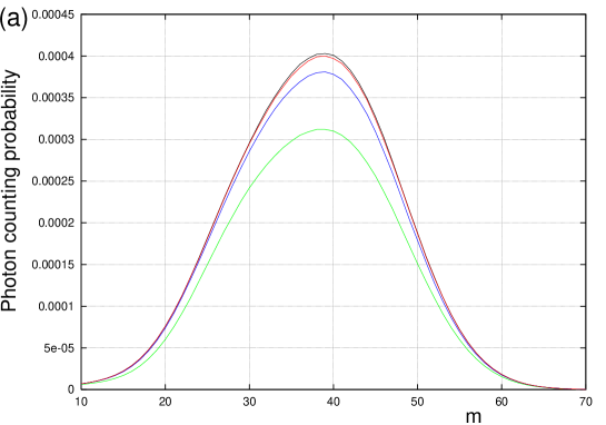
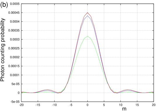
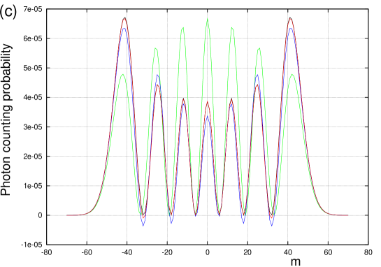
Figure 3: The simulation for (a) coherent state $|\gamma\rangle$ with $\gamma=2$ for $j=190$, (b) squeezed state with squeezing parameter $r=1.5$ for $j=219.5$, and (c) number state $|6\rangle$ for $j=183.5$. The exact probabilities are shown in black, and the truncated ones are shown in green, blue and red, respectively, according to the increasing number of terms in Eq. (37) taken into account. The red curves are so close to the black ones in (b) and (c) that they almost cover them in the plots.

The LO amplitude was chosen to be $\alpha=-A=-20$ which means that the mean photon number of the LO field is 400. The value of $j$ in the individual plots was chosen randomly from the Poissonian distribution of LO photon number. It has turned out during the simulations that changing $j$ inside the interval for which the probability $P^{j}_{m}$ is non-negligible does not affect the behavior of the series significantly. As the signal states we have chosen a coherent state with amplitude $2$, a squeezed vacuum state Rad87 $\exp[r(\hat{a}^{2}-\hat{a}^{\dagger 2})/2]\,|0\rangle$ with $r=1.5$ and a number state $|6\rangle$. The results of the simulations are shown in Fig. 3. The exact probabilities $P^{j}_{m}$ are shown in black, and the results of truncation of the series (37) keeping terms with (i) zero number of field operators,

$$P_{m}^{j\,(0)}=\frac{\sqrt{\pi}\,2^{-2j}\,e^{-A^{2}}\,A^{4j}\,e^{2m^{2}/A^{2}}}{(j+m)!\,(j-m)!}\,\langle x|\hat{\rho}|x\rangle,$$ (43)

are shown in green color, (ii) maximum of two field operators

$$P_{m}^{j\,(2)}=\frac{\sqrt{\pi}\,2^{-2j}\,e^{-A^{2}}\,A^{4j}\,e^{2m^{2}/A^{2}}}{(j+m)!\,(j-m)!}\,\left\{\langle x|\hat{\rho}|x\rangle-\frac{2j-A^{2}}{2A^{2}}[\langle x|\hat{a}^{2}\hat{\rho}|x\rangle+\langle x|\hat{\rho}(\hat{a}^{\dagger})^{2}|x\rangle]\right\}$$ (44)

are shown in blue color, and (iii) maximum of four field operators are shown in red (we do not write $P_{m}^{j\,(4)}$ explicitly).

The simulations show that with increasing number of terms in the series (37), a better approximation to the exact photon counting probability is achieved.

V Conclusion

We have analyzed balanced homodyne detection in terms of the POVM for photon counting by directly calculating the photon counting probability. We employed two different approaches. First, using asymptotic expressions for SU(2) Wigner functions allowed us to establish the non-trivial connection between the discrete variables $j,m$ corresponding to photon numbers being detected and the continuous quadrature phase variable $x_{\varphi}$. In the strong LO limit, we have shown that homodyne detection indeed performs the projective measurements corresponding to POVM $|x\rangle\langle x|$, where $|x\rangle$ is the eigenstate of quadrature phase operator. Second, employing the Glauber-Sudarshan $P$-function, we extended the result obtained by the first approach. For a very large amplitude of the LO, the result was the same, and for finite amplitudes we obtained additional correction terms. Even though the series we got does not converge in general, it can be used for determining the correction terms via truncation of the signal state in the Fock basis. We have determined the strong LO condition for coherent and number signal states – the square of the mean photon number in the signal state must be much smaller than the mean photon number in the LO. We have also performed numerical simulations that confirm the validity of the quadrature-phase POVM and the correction terms for a LO that is not strong for typical signal states. Therefore, in addition to obtaining the quadrature-phase POVM rigorously from the photon counting POVM, we have an expansion that yields correction terms for the POVM that works well for typical signal states in quantum optics.

In this paper we have considered a perfect HD scheme with ideal detectors, LO and BS and 100% mode-matching. In practice, all these elements are subject to imperfections, which disturbs the measurement. For example, the LO from a realistic laser has an amplitude distribution $P_{\rm LO}(\alpha)$ broader than the delta-function. This would convolute the probability $P^{j}_{m}(\alpha)$, where we now write the dependence on $\alpha$ explicitly, with $P_{\rm LO}(\alpha)$. If this distribution is Gaussian, then the strong LO measurement would correspond to a Gaussian spread of the quadrature measurement with the imprecision corresponding to the degree of LO amplitude fluctuation. Lossy beamsplitters and inefficient photodetectors would add vacuum noise that would result in Gaussian spread of quadrature measurement, similar to the effect discussed above for the LO amplitude spread. Finally, for a multi-mode field with the LO mode-matching condition satisfied, the detection efficiency can incorporate the mismatch between the beam and detector modes. If, on the other hand, the signal and LO modes are mismatched, HD efficiency declines, and beats between different frequency modes arise.

Our operational approach to HD ignores the realistic effects described above, but the theory is readily generalized to accommodate these effects by including inefficiencies and multimode description. Moreover, if multimode fields and beats are desirable, heterodyne detection replaces homodyne detection (for which signal and LO are frequency matched); an operational formulation of heterodyne detection without mean field approximation is a topic of further research.

Appendix A Properties of the P representation for $z$–regular states

We first prove Lemma 1 for pure $z$–regular states and then generalize to mixed states. The density operator associated with a normalized pure state $|\psi\rangle$ is

$$\hat{\rho}=|\psi\rangle\langle\psi|,$$ (45)

and is represented by the Glauber-Sudarshan P representation according to Eq. (23). The trace of $\hat{\rho}$ is unity due to the normalization of the state $|\psi\rangle$ and hence the integral of the $P$–function over the complex plane is equal to unity:

$$\int P(\beta)\,{\rm d}^{2}\beta=\int P(\beta){\rm Tr}\,|\beta\rangle\langle\beta|\,{\rm d}^{2}\beta={\rm Tr}\,\hat{\rho}=1.$$ (46)

Now, for a positive number $r$ we define a non-unitary operator

$$\hat{S}(r)={\rm e}^{-r}\,\exp\left(\frac{r\hat{a}}{z}\right)$$ (47)

and, for a normalized $z$-regular state $|\psi\rangle$ [see Eq. (27)], we consider the state

$$|\psi^{\prime}\rangle=\hat{S}(r)|\psi\rangle={\cal N}\sum_{n=0}^{\infty}\frac{c^{\prime}_{n}z^{n}}{\sqrt{n!}}\,|n\rangle,$$ (48)

where the coefficients $c^{\prime}_{n}$ are related to the coefficients $c_{n}$ by

$$c_{n}^{\prime}={\rm e}^{-r}\,\sum_{m=0}^{\infty}\frac{c_{n+m}r^{m}}{m!}=\frac{\sum_{m=0}^{\infty}c_{n+m}r^{m}/m!}{\sum_{m=0}^{\infty}r^{m}/m!}.$$ (49)

Clearly $|c^{\prime}_{n}|\leq 1$, so the state $|\psi^{\prime}\rangle$ is also $z$ regular but generally not normalized. To normalize it, we introduce the inverse norm ${\cal N^{\prime}}=\langle\psi^{\prime}|\psi^{\prime}\rangle^{-1/2}$ so that the state $|\psi^{\prime}\rangle_{N}={\cal N^{\prime}}|\psi^{\prime}\rangle=\langle\psi^{\prime}|\psi^{\prime}\rangle^{-1/2}|\psi^{\prime}\rangle$ is normalized. The density operator $\hat{\rho}^{\prime}$ of $|\psi^{\prime}\rangle_{N}$ can be expressed via the density operator $\hat{\rho}$ as

$$\hat{\rho}^{\prime}={\cal N^{\prime}}^{2}{\rm e}^{-2r}\,\exp\left(\frac{r\hat{a}}{z}\right)\hat{\rho}\exp\left(\frac{r\hat{a}^{\dagger}}{z}\right)$$ (50)

and the P function corresponding to $|\psi^{\prime}\rangle_{N}$ is hence

$$P^{\prime}(\beta)={\cal N^{\prime}}^{2}{\rm e}^{-2r}\,\exp\left(\frac{r\beta}{z}\right)\exp\left(\frac{r\beta^{*}}{z}\right)\,P(\beta)={\cal N^{\prime}}^{2}\exp\left[2r\left(\frac{{\rm Re\,}\beta}{z}-1\right)\right]\,P(\beta).$$ (51)

The integral of $P^{\prime}$ over the complex plane is unity as the state $|\psi^{\prime}\rangle_{N}$ is normalized:

$$\int P^{\prime}(\beta)\,{\rm d}^{2}\beta=1$$ (52)

Decomposing $\beta$ to real and imaginary parts $\beta=\beta_{1}+{\rm i}\beta_{2}$, and using Eq. (51), we can write Eq. (52) as a double integral

$$1 = {\cal N^{\prime}}^{2}\,\int_{-\infty}^{\infty}\,{\rm d}\beta_{1}\,\exp\left[2r\left(\frac{\beta_{1}}{z}-1\right)\right]\int_{-\infty}^{\infty}\,{\rm d}\beta_{2}P(\beta_{1},\beta_{2})$$ (53)

$$= {\cal N^{\prime}}^{2}\,\int_{-\infty}^{\infty}\exp\left[2r\left(\frac{\beta_{1}}{z}-1\right)\right]\,G(\beta_{1})\,{\rm d}\beta_{1},$$

where we have denoted

$$G(\beta_{1})=\int_{-\infty}^{\infty}P(\beta_{1},\beta_{2})\,{\rm d}\beta_{2}.$$ (54)

The inner product $\langle\psi^{\prime}|\psi^{\prime}\rangle$ can be bound as follows [see Eq. (48)]:

$$\langle\psi^{\prime}|\psi^{\prime}\rangle={\cal N^{\prime}}^{-2}={\cal N}^{2}\sum_{n=0}^{\infty}\frac{|c^{\prime}_{n}|^{2}z^{2n}}{n!}\leq{\cal N}^{2}\sum_{n=0}^{\infty}\frac{z^{2n}}{n!}={\cal N}^{2}{\rm e}^{z^{2}}.$$ (55)

From Eqs. (53) and (55),

$$\int_{-\infty}^{\infty}\exp\left[2r\left(\frac{\beta_{1}}{z}-1\right)\right]\,G(\beta_{1})\,{\rm d}\beta_{1}\leq{\cal N}^{2}{\rm e}^{z^{2}}.$$ (56)

We see that the integral (56) is bound by a fixed number ${\cal N}^{2}{\rm e}^{z^{2}}$, no matter how large $r$ we choose. The only way to satisfy this is if $G(\beta_{1})\equiv 0\,\,\forall\beta_{1}>z$. Specifically if $f(x):\mathbb{R}\to\mathbb{R}$ is a function and we know that

$$\int_{-\infty}^{\infty}f(x)\,{\rm e}^{ax}\,{\rm d}x<c$$ (57)

where $c>0$ is fixed and $a$ is arbitrary positive, then necessarily $f(x)=0$ for all $x>0$. Thus, we obtain

$$G(\beta_{1})=\int_{-\infty}^{\infty}P(\beta_{1},\beta_{2})\,{\rm d}\beta_{2}=0\quad{\rm for}\quad\beta_{1}>z,$$ (58)

which means that the integral of $P$ over any vertical line in the complex plane that is farther than $z$ from the origin is zero.

Now the whole construction can be repeated with another state

$$|\psi^{\prime}_{\varphi}\rangle={\rm e}^{-r}\,\exp\left(\frac{re^{{\rm i}\varphi}\hat{a}}{z}\right)|\psi\rangle$$ (59)

whose P function is

$$P^{\prime}_{\varphi}(\beta)=\langle\psi^{\prime}_{\varphi}|\psi^{\prime}_{\varphi}\rangle^{-1}\exp\left[2r\left(\frac{{\rm Re\,}(\beta e^{{\rm i}\varphi})}{z}-1\right)\right]\,P(\beta).$$ (60)

Using the same argument, we arrive at the fact that the integral of $P(\beta)$ over any line whose normal has the angle $\varphi$ with the real axis and whose distance from the origin is larger than $z$ (eg the line $l$ in Fig. 2) is zero. Now, as $\varphi$ can be arbitrary, this means that the integral over all lines not intersecting the circle with radius $z$ is zero. Then it follows by the tomographic argument that the P-function must be zero outside the circle, which is what we wanted to prove.

Figure 2: The integral of the P function of the state $|\psi\rangle$ over the line $l$ shown in the picture vanishes, and so it does for all other lines that do not intersect the circle $|\beta|=z$. Therefore the P function itself vanishes outside the circle, i.e., for $|\beta|>z$.

The generalization of the claim to mixed $z$ regular states is straightforward as the P-function of a mixed state is the weighed sum of the P-functions of the pure states in the mixture.

Appendix B Proof of Lemma 2

A direct calculation yields

$${\rm Tr}\,\left(\hat{\rho}\,(\hat{a}^{\dagger})^{n}|x\rangle\langle x|\,\hat{a}^{m}\right)\hat{\rho} = \int P(\gamma)\,\langle x|\,\hat{a}^{m}|\gamma\rangle\langle\gamma|(\hat{a}^{\dagger})^{n}\,|x\rangle\,{\rm d}^{2}\gamma$$ (61)

$$= \int P(\gamma)\,\gamma^{m}(\gamma^{*})^{n}|\langle x|\gamma\rangle|^{2}\,{\rm d}^{2}\gamma$$

$$= \frac{1}{\sqrt{\pi}}\int P(\gamma)\,\gamma^{m}(\gamma^{*})^{n}e^{-[2^{-1/2}(\gamma+\gamma^{*})-x]^{2}}\,{\rm d}^{2}\gamma.$$

Here the fact that $|\langle x|\gamma\rangle|^{2}=\pi^{-1/2}\exp[-(x-\sqrt{2}\,{\rm Re\{\gamma\})^{2}]}$ was used.

References

- (1) Radmore P M and Barnett S M 1997 Methods in Theoretical Quantum Optics (Oxford University Press)
- (2) Yuen H P and Shapiro J H 1978 in Coherence and Quantum Optics IV (Plenum, New York) 719.
- (3) Yuen H P and Shapiro J H 1979 IEEE Trans. Inf. Theory IT-25 179; Yuen H P and Shapiro J H 1980 IEEE Trans. Inf. Theory IT-26 78
- (4) Yuen H P and Chan V W 1983 Opt. Lett. 8 177; Yuen H P and Chan V W 1983 8 345(E); Schumaker B L 1984 Opt. Lett. 9 189
- (5) Glauber R J 1963 Phys. Rev. 131 2766
- (6) Sudarshan E C G 1963 Phys. Rev. Lett. 10 277
- (7) Vogel K, Risken H 1989 Phys. Rev. A 40 2847; Paul H, Leonhardt U and D’Ariano G M 1995 Acta Phys. Slov. 45 261
- (8) Vaidman L 1994 Phys. Rev. A 49 1473
- (9) Braunstein S L and Kimble H J 1998 Phys. Rev. Lett. 80 869
- (10) Furusawa A, Sørensen J L, Braunstein S L,Fuchs C A, Kimble H J and Polzik E S 1998 Science 282 706
- (11) N. G. Walker, J. Mod. Optics 34, 15 (1987).
- (12) Braunstein S L 1990 Phys. Rev. A 42 474
- (13) Banaszek K and Wódkiewicz K 1997 Phys. Rev. A 55 3117
- (14) Rudolph T and Sanders B C 2001 Phys. Rev. Lett. 87 077903; Sanders B C, Bartlett S D, Rudolph T and Knight P L 2003 Phys. Rev. A 68 042329
- (15) Schumaker B L 1986 Phys. Rep. 135 317–408
- (16) Mølmer K 1997 Phys. Rev. A 55 3195; Mølmer K 1997 J. Mod. Opt. 44 1937; Gea-Banacloche J. 1998 Phys. Rev. A 58 4244; Mølmer K 1998 Phys. Rev. A 58 4247
- (17) Yurke B, McCall S L and Klauder J R 1986 Phys. Rev. A 33 4033
- (18) Campos R A, Saleh B E A and Teich M C 1989 Phys. Rev. A 40 1371
- (19) Sanders B C and Milburn G J 1995 Phys. Rev. Lett. 75 2944
- (20) Rowe D J, Sanders B C and de Guise H 2001 J. Math. Phys. 42 2315
- (21) Susskind L and Glogower J 1964 Physics 1 49
- (22) Glauber R J 1963 Phys. Rev. Lett. 10 84
- (23) Klauder J R and Sudarshan E C G 1968 Fundamentals of Quantum Optics (Benjamin, New York)