Completely Positive Post-Markovian Master Equation via a Measurement Approach

Abstract

A new post-Markovian quantum master equation is derived, that includes bath memory effects via a phenomenologically introduced memory kernel $k(t)$. The derivation uses as a formal tool a probabilistic single-shot bath-measurement process performed during the coupled system-bath evolution. The resulting analytically solvable master equation interpolates between the exact Nakajima-Zwanzig equation and the Markovian Lindblad equation. A necessary and sufficient condition for complete positivity in terms of properties of $k(t)$ is presented, in addition to a prescription for the experimental determination of $k(t)$. The formalism is illustrated with examples.

An open quantum system is one that is coupled to an external environment Breuer:book ; Alicki:87 . Such systems are of fundamental interest, as the notion of a closed system is always an idealization and approximation. Open quantum systems tend to decohere, and for this reason have recently received intense consideration in quantum information science, where decoherence is viewed as fundamental obstacle to the construction of quantum information processors Nielsen:book . It is possible to write down an exact dynamical equation for an open system, but the result – an integro-differential equation Nakajima:58Zwanzig:60a – is mostly of formal interest, as such an exact equation can almost never be solved analytically or even numerically. In contrast, when one makes the Markovian approximation, i.e., when one neglects all bath memory effects, the resulting Lindblad master equation Gorini:76Lindblad:76 ; Alicki:87 is formally solvable and amenable to numerical treatment. Moreover, the desirable property of complete positivity Kraus:83 is maintained (see, however, Pechukas:94Pechukas+Alicki:95 for a debate on the importance of this property). A coveted goal of the theory of open quantum systems Breuer:book ; Alicki:87 is a “post-Markovian” master equation that (i) generalizes the Markovian Lindblad equation so as to include bath memory effects, at the same time (ii) remains both analytically and numerically tractable, and (iii) retains complete positivity. A variety of post-Markovian master equations have been proposed and analyzed, e.g., Breuer:book ; Shibata:77Chaturvedi:79 ; Imamoglu:94 ; Royer:96Royer:03 ; Garraway:97Breuer:99knezevic:012104 ; gambetta:012108breuer:022115 ; Strunz:99Yu:2000 ; barnett:033808 ; Daffer:03 ; Breuer:04 . However, one of the desirable properties (i)-(iii) above is typically lost: e.g., in the case of time-convolutionless master equations (e.g., Royer:96Royer:03 ) one may lose complete positivity, while in the case of nonlocal stochastic Schrodinger equations (e.g., Strunz:99Yu:2000 ) one loses analytical solvability. In this work we propose a new post-Markovian master equation that satisfies all of the desirable properties (i)-(iii) above. The key idea we introduce is an interpolation between the generalized measurement interpretation of the exact Kraus operator sum map Kraus:83 , and the continuous measurement interpretation of Markovian-limit dynamics Dalibard:92Gisin:92Plenio:98 ; Breuer:04 .

Review of quantum measurements approach to open system dynamics.— Consider a quantum system $S$ coupled to a bath $B$ (with respective Hilbert spaces $\mathcal{H}_{S},\mathcal{H}_{B}$), evolving unitarily under the total system-bath Hamiltonian $H_{SB}$. The exact system dynamics is given by tracing over the bath degrees of freedom Breuer:book ; Alicki:87 ; Nielsen:book

$$\rho(t)=\mathrm{Tr}_{B}[U(t)\rho_{SB}(0)U^{{\dagger}}(t)],$$ (1)

where $\rho(t)$ is the system state, $\rho_{SB}(0)=\rho(0)\otimes\rho_{B}(0)$ is the initially uncorrelated system-bath state, and $U(t)=\mathcal{T}\mathsf{\exp}(-i\int_{0}^{t}H_{SB}(t^{\prime})dt^{\prime})$ ($\mathcal{T}$ denotes time-ordering; we set $\hbar=1$ and for simplicity work in the interaction picture with respect to both system and bath). Eq. (1) can be rewritten in terms of an operator sum (the Kraus representation Kraus:83 )

$$\rho(t)=\sum_{k}A_{k}^{{\dagger}}(t)\rho(0)A_{k}(t),$$ (2)

where $\mathrm{Tr}[\rho(t)]=1\Leftrightarrow\sum_{k}A_{k}(t)A_{k}^{{\dagger}}(t)=I$.

Let us now recall how to derive the exact Eq. (1) from a measurement picture [Fig. 1a]. Imagine the bath acting as a probe coupled to the system at $t=0$, with the interaction given by $H_{SB}$ as above. To study the state of the system a single projective measurement is performed on the bath at time $t$, with a complete set of projection operators $|i\rangle\langle i|$, $\mathcal{H}_{B}=\mathrm{Span}\{|i\rangle\}$. The measurement yields the result $k$ and collapses the state of the bath to the corresponding eigenstate $|k\rangle$. This happens with probability $p_{k}=\mathrm{Tr}_{S}[\langle k|\rho_{SB}(t)|k\rangle]$, and the system density matrix reduces to $\rho^{k}(t)=\langle k|\rho_{SB}(t)|k\rangle/p_{k}=:A_{k}^{{\dagger}}\rho(0)A_{k}/p_{k}$, where $A_{k}$ are the Kraus operators. If we repeat this process for an identical ensemble initially prepared in state $\rho_{SB}(0)$ the average system density matrix becomes $\rho(t)=\sum_{k}p_{k}\rho^{k}(t)=\mathrm{Tr}_{B}[U(t)\rho_{SB}(0)U^{{\dagger}}(t)]$, which is just Eq. (1), thus affirming the validity of this bath-measurement interpretation of open system dynamics. The corresponding map $\Phi$ is completely positive (CP) CP .

In contrast, in the Markovian limit the most general CP system dynamics is given in the interaction picture by the Lindblad equation Gorini:76Lindblad:76

$$\frac{\partial\rho}{\partial t}=\mathcal{L}\rho:=-\frac{1}{2}\sum_{a}a_{\alpha}([F_{\alpha},\rho F_{\alpha}^{{\dagger}}]+[F_{\alpha}\rho,F_{\alpha}^{{\dagger}}]).$$ (3)

The Lindblad operators $F_{\alpha}$’s are bounded operators acting on $\mathcal{H_{S}}$, and the $a_{\alpha}\geq 0$ are constants that describe decoherence rates. Now let us recall how also the Lindblad equation can be given a measurement interpretation. Expanding Eq. (3) to first order in the short time interval $\tau$ yields $\rho(t+\tau)=(I-\frac{\tau}{2}\sum_{\alpha}F_{\alpha}^{{\dagger}}F_{\alpha})\rho(t)(I-\frac{\tau}{2}\sum_{\alpha}F_{\alpha}^{{\dagger}}F_{\alpha})+\tau\sum_{\alpha}F_{\alpha}\rho(t)F_{\alpha}^{{\dagger}}$. To the same order we also have the normalization condition $(I-\frac{\tau}{2}\sum_{\alpha}F_{\alpha}^{{\dagger}}F_{\alpha})(I-\frac{\tau}{2}\sum_{\alpha}F_{\alpha}^{{\dagger}}F_{\alpha})+\tau\sum_{\alpha}F_{\alpha}^{{\dagger}}F_{\alpha}=I$. Thus the Lindblad equation has been recast as a Kraus operator sum (2), but only to first order in $\tau$, the coarse-graining time scale for which the Markovian approximation is valid Lidar:CP01 . Clearly, then, we again have a measurement interpretation, wherein as before the bath functions as a probe coupled to the system while being subjected to a continuous series of measurements at each infinitesimal time interval $\tau$ [Fig. 1b)]. This is the well-known quantum jump process Dalibard:92Gisin:92Plenio:98 , wherein the measurement operators are $I-\frac{\tau}{2}\sum_{\beta}F_{\beta}^{{\dagger}}F_{\beta}$ (the “conditional” evolution) and $\sqrt{\tau}F_{\alpha}$ (the “jump”).

We have thus seen how a measurement picture leads to the two limits of exact dynamics (via an evolution of the coupled system-bath followed by a single generalized measurement at time $t$), and Markovian dynamics (via a series of measurements interrupting the joint evolution after each time interval $\tau$). With this in mind it is now easy to see that by relaxing the many-measurements process one is led to a less restricted approximation than the Markovian one. Here we use this observation to derive a post-Markovian master equation based on a probabilistic single-shot measurement process.

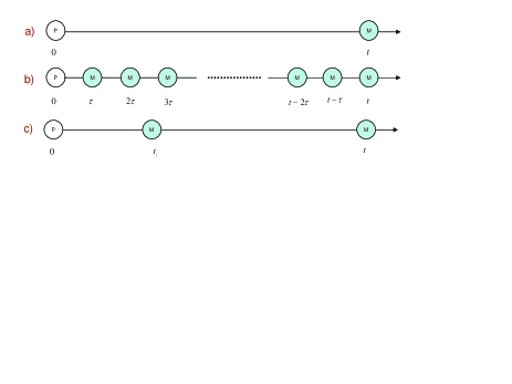
Figure 1: Measurement approach to open system dynamics. P$=$preparation, M$=$ measurement, time proceeds from left to right. a) Exact Kraus operator sum representation, b) Markovian approximation, c) Single-shot measurement, d) Single-shot measurement followed by Markovian dynamics.

Derivation of a post-Markovian master equation.— The first stage of exerting an approximation on the exact Eq. (1) should be to include one extra measurement in the time interval $[0,t]$. Thus we consider the following process: a probe (bath) is coupled to the system at $t=0$, they evolve jointly for a time $t^{\prime}$ ($0\leq t^{\prime}<t$) such that at $t^{\prime}$ the system state is $\Lambda(t^{\prime})\rho(0)$, where $\Lambda(t^{\prime})$ is a one-parameter map, at which moment the extra generalized measurement is performed on the bath. $\Lambda$ does not depend on $t$ since the bath resets upon measurement. System and bath continue their coupled evolution between $t^{\prime}$ and $t$, upon which the final measurement is applied. This is illustrated in Fig. 1c. Since this intermediate measurement determines the system state $|\psi\rangle$ at $t^{\prime}$, after time $t-t^{\prime}$ the system state will be $\rho(t)=\Lambda(t-t^{\prime})\rho(t^{\prime})$. It is important to stress that $\rho(t^{\prime})$ cannot be written as $\Lambda(t^{\prime})\rho(0)$, since the measurement selects $\rho(t^{\prime})$ at random.

The time $t^{\prime}$ characterizes bath memory effects and must be determined as a function of time-scales characterizing the evolution. We do this by introducing a bath memory function (kernel) $k(t-t^{\prime},t)$ that assigns weights to different measurements. To derive a master equation we discretize the time interval $[0,t]$ into $N$ equal segments of length $\epsilon$, and express $t=N\epsilon,t^{\prime}=m\epsilon$. We then have the weighted average $\rho(t=N\epsilon)=\sum_{m=1}^{N}k((N-m)\epsilon,N\epsilon)\Lambda((N-m)\epsilon)\rho(m\epsilon)=\sum_{m=1}^{N}k(m\epsilon,N\epsilon)\Lambda(m\epsilon)\rho((N-m)\epsilon)$. From hereon we assume that $\Lambda$ is trace-preserving, whence $k$ must be normalized so that $\sum_{m=1}^{N}k(m\epsilon,N\epsilon)=1$ ($k(t^{\prime},t)=0$ for $t^{\prime}\notin[0,t]$), though an exception to this will arise below. We then have (for $N\geq 1$)

$$\rho(N\epsilon)-\rho((N-1)\epsilon)=\sum_{m=1}^{N-1}k(m\epsilon,(N-1)\epsilon)\Lambda(m\epsilon)\times$$

$$[\rho((N-m)\epsilon)-\rho((N-m-1)\epsilon)]+\sum_{m=1}^{N-1}[k(m\epsilon,N\epsilon)$$

$$-k(m\epsilon,(N-1)\epsilon)]\Lambda(m\epsilon)\rho((N-m)\epsilon)$$

$$+k(N\epsilon,N\epsilon)\Lambda(N\epsilon)\rho(0).$$ (4)

In order to arrive at a differential equation the term proportional to $\Lambda(N\epsilon)\rho(0)$ must be made to vanish. We therefore impose the additional constraint $\lim_{\epsilon\rightarrow 0}k(N\epsilon,N\epsilon)/\epsilon=0$. Taking the limits $\epsilon\rightarrow 0$, $m,N\rightarrow\infty$ such that $m\epsilon=t^{\prime}$ and $N\epsilon=t$, we convert the remaining terms in Eq. (4) into differential form by expressing $[\rho((N-m)\epsilon)-\rho((N-1-m)\epsilon)]/\epsilon\rightarrow\frac{\partial\rho(t-t^{\prime})}{\partial(t-t^{\prime})}$ and $[k(m\epsilon,N\epsilon)-k(m\epsilon,(N-1)\epsilon)]/\epsilon\rightarrow\frac{\partial k(t^{\prime},t)}{\partial t}$. Eq. (4) then yields: $\frac{\partial\rho}{\partial t}=\int_{0}^{t}dt^{\prime}[k(t^{\prime},t)\Lambda(t^{\prime})\frac{\partial\rho(t-t^{\prime})}{\partial(t-t^{\prime})}+\frac{\partial k(t^{\prime},t)}{\partial t}\Lambda(t^{\prime})\rho(t-t^{\prime})]$. We would like to arrive at a proper integro-differential equation involving, on the right-hand-side (RHS), only $\rho$ and not its derivative. We thus assume, only in the derivative of $\rho$ on the RHS, that $\rho(t-t^{\prime})=\Lambda(t-t^{\prime})\rho(0)$. Such an assumption is equivalent to the standard procedure of first-order time-dependent perturbation theory, and can, analogously, be iterated self-consistently to obtain higher-order approximations. Expressing $\rho(0)=\Lambda^{-1}(t-t^{\prime})\rho(t-t^{\prime})$ we then obtain the post-Markovian dynamical equation

$$\frac{\partial\rho}{\partial t} = \int_{0}^{t}dt^{\prime}[k(t^{\prime})\Lambda(t^{\prime})\dot{\Lambda}(t-t^{\prime})\Lambda^{-1}(t-t^{\prime})$$ (5)

$$+\frac{\partial k(t^{\prime},t)}{\partial t}\Lambda(t^{\prime})]\rho(t-t^{\prime}).$$

This new, formal master equation is the first main result of this work. Note that in this integral form the constraint $\lim_{\epsilon\rightarrow 0}k(N\epsilon,N\epsilon)/\epsilon=0$ can be lifted, as it cannot change the value of the integral.

To make further progress we now assume a Markovian form for the superoperator: $\Lambda(t)=\exp(\mathcal{L}t)$. Here $\mathcal{L}$ can be interpreted as the Lindblad generator [Eq. (3)]. Using this in Eq. (5) yields

$$\frac{\partial\rho}{\partial t}=\int_{0}^{t}dt^{\prime}[k(t^{\prime},t)\mathcal{L}+\frac{\partial k(t^{\prime},t)}{\partial t}]\exp(\mathcal{L}t^{\prime})\rho(t-t^{\prime}).$$ (6)

This master equation is rather interesting and appears amenable to analytical treatment, an undertaking which will be the subject of a future study. To make even further progress, let us note that Eq. (6) automatically preserves $\mathrm{Tr}\rho$, even without requiring normalization of $k$ via $\int_{0}^{t}k(t^{\prime},t)dt^{\prime}=1$. Since the latter was needed above to ensure trace preservation, it can now be dropped. This allows us to consider memory kernels satisfying $k(t^{\prime},t)=k(t^{\prime})$. We thus arrive at our second main result:

$$\frac{\partial\rho}{\partial t}=\mathcal{L}\int_{0}^{t}dt^{\prime}k(t^{\prime})\exp(\mathcal{L}t^{\prime})\rho(t-t^{\prime})=\mathcal{L}k(t)\exp(\mathcal{L}t)\ast\rho(t),$$ (7)

where $\ast$ denotes convolution and $k$ no longer obeys any constraints.

Henceforth we confine our attention for simplicity and explicitness to the new post-Markovian master equation (7), though some of the results below are generalizable to Eq. (5). While $k$ is still unspecified, we show below that it can be determined by an appropriate quantum state tomography experiment. As we further show below, Eq. (7) satisfies all the conditions we stated in the introduction for a “desirable” post-Markovian master equation. Finally, note that Eq. (7) reduces to a purely Markovian master equation, ${\partial\rho}/{\partial t}=\mathcal{L}\rho(t)$, when $k(t^{\prime})=\delta(t^{\prime})$, as expected for a memoriless channel.

Dynamical map.— We now analytically derive the dynamical map $\Phi(t):\rho(0)\mapsto\rho(t)$ governing our master equation. We solve the integro-differential equation (7) by taking the Laplace transform:

$$s\widetilde{\rho}(s)-\rho(0)=[\widetilde{k}(s)\ast\frac{\mathcal{L}}{s-\mathcal{L}}]\widetilde{\rho}(s),$$ (8)

where $\widetilde{X}(s):=\mathsf{Lap}[X(t)]$ is the Laplace transform of the function $X(t)$. Now consider the solution of the eigenvalue equation $\mathcal{L}\rho=\lambda\rho$. It results in a set of (complex) eigenvalues $\{\lambda_{i}\}$ and corresponding right and left eigenvectors $\{R_{i}\},\{L_{i}\}$ that fulfill the orthonormality condition $\mathrm{Tr}[L_{i}R_{j}]=\delta_{ij}$. These eigenvectors are known as the damping basis Briegel:93 of the superoperator $\mathcal{L}$. Expressing the density matrix in this basis as $\rho(t)=\sum_{i}\mathrm{Tr}[L_{i}\rho(t)]R_{i}=\sum_{i}\mu_{i}(t)R_{i}$ and taking the Laplace transform, allows us to use Eq. (8) to solve for the expansion functions $\mu_{i}(t)$: $s\widetilde{\mu}_{i}(s)-\mu_{i}(0)=\lambda_{i}\widetilde{k}(s-\lambda_{i})\widetilde{\mu}_{i}(s)\implies$

$$\mu_{i}(t)=\mathsf{Lap}^{-1}[\frac{1}{s-\lambda_{i}\widetilde{k}(s-\lambda_{i})}]\mu_{i}(0)=:\xi_{i}(t)\mu_{i}(0).$$ (9)

The functions $\xi_{i}(t)$ can now be computed using the residue theorem formula applied to the Bromwich integral formula for the inverse Laplace transform: if $f(s)=\mathsf{Lap}[F(t)]$ then $F(t)=\sum_{p_{k}}\mathrm{Res}[e^{st}f(s),p_{k}]$, where $p_{k}$ are the poles of $e^{st}f(s)$ and $\mathrm{Res}[g,p]:=\frac{1}{(n-1)!}\left(\frac{d^{n-1}}{ds^{n-1}}[(s-p)^{n}g(s)]\right)_{s=p}$ is the residue of $g$, with $n$ the order of the pole $p$. In our case $f(s)=[s-\lambda_{i}\widetilde{k}(s-\lambda_{i})]^{-1}$ and so the poles $p_{k}$ are determined by the solutions of the equation $s=\lambda_{i}\widetilde{k}(s-\lambda_{i})$ for $s$. This equation can be solved once the Lindblad generator $\mathcal{L}$ (yielding the $\lambda_{i}$) and the memory kernel $k(t)$ are specified. Then $\xi_{i}(t)=\sum_{p_{k}^{(i)}}\mathrm{Res}[e^{st}f(s),p_{k}^{(i)}]$. Summarizing, the dynamical map corresponding to Eq. (7) is

$$\Phi(t):X\mapsto\sum_{i}\xi_{i}(t)\mathrm{Tr}[L_{i}X]R_{i}.$$ (10)

Using the orthonormality of the damping basis it follows that $\Phi(t)^{-1}:Y\mapsto\sum_{i}\xi_{i}(t)^{-1}\mathrm{Tr}[L_{i}Y]R_{i}$. Thus $\Phi$ is invertible with the exception of the points where $\xi_{i}(t)=0$. For contractive (e.g., Markovian) maps this will happen at $t=\infty$, though in general additional points cannot be excluded.

Condition for complete positivity of $\Phi$.— Let us recall Choi’s theorem Choi:75 : “Let $\Psi:GL(n;\mathbb{C})\mapsto GL(m;\mathbb{C})$ be a linear map. Then $\Psi$ is CP iff  the matrix whose elements are $\{\Psi[E_{ij}]\}_{1\leq i,j\leq n}$ is positive, where $E_{ij}$ is a matrix with $(E_{ij})_{i,j}=1$ and all other elements zero.” Using Choi’s theorem Choi:75 the criterion for complete positivity of our map is equivalent to positivity of the matrix $P$ whose $(i,j)$th element is $\Phi[|i\rangle\langle j|]$. Namely, $P\geq 0\Leftrightarrow\{\sum_{k}\xi_{k}(t)\mathrm{Tr}[L_{k}|i\rangle\langle j|]R_{k}\}_{1\leq i,j\leq n}=\{\sum_{k}\xi_{k}(t)\langle j|L_{k}|i\rangle R_{k}\}_{1\leq i,j\leq n}\geq 0$, which, in turn, is equivalent to:

$$\sum_{k}\xi_{k}(t)L_{k}^{T}\otimes R_{k}\geq 0.$$ (11)

The inequality (11) is a necessary and sufficient condition for our map to be CP. Because the functions $\xi_{k}(t)$ are given in terms of the memory kernel $k(t)$ through Eq. (9), this inequality results in a condition on $k(t)$, which can be checked in order to verify that a given such kernel results in a CP map. Further note that Eq. (7) preserves the trace of $\rho(t)$ [i.e., $d\mathrm{\ Tr}\rho(t)/dt=0$], as is evident from $\mathrm{Tr}\mathcal{L}=0$ and a Taylor expansion of $\exp(\mathcal{L}t)$.

Kraus representation of $\Phi$.— Since the matrix $P$ is positive it can be expressed as $P=\sum_{k}|a_{k}\rangle\langle a_{k}|$ where the $|a_{k}\rangle$’s are the eigenvectors of $P$. One can divide the vector $|a_{k}\rangle$ into $n$ segments of length $n$, where $n=\dim[\mathcal{H}_{S}]$, and define a matrix $M_{k}$ with the $i$th column being the $i$th segment of $|a_{k}\rangle$, so that the $i$th segment is $M_{k}|i\rangle$. Then the dynamical map is reconstructed as $\mathcal{E}(\rho)=\sum_{\alpha}M_{\alpha}\rho M_{\alpha}^{{\dagger}}$, which is the desired Kraus representation.

Connection to other master equations.— We first note that our master equation (7) is an instance of the exact Nakajima-Zwanzig (NZ) equation $\overset{.}{\rho}=\int_{0}^{t}dt^{\prime}O(t,t^{\prime})\rho(t^{\prime})$ Nakajima:58Zwanzig:60a , where the NZ kernel $O(t,t^{\prime})$ is, in our case, of the special time translationally-invariant form $O(t^{\prime}-t)$. Secondly, in the particular case that $||\mathcal{L}||\ll 1/t$ Eq. (7) reduces to

$$\frac{\partial\rho}{\partial t}=\mathcal{L}\int_{0}^{t}dt^{\prime}k(t^{\prime})\rho(t-t^{\prime}).$$ (12)

This master equation was proposed intuitively in Ref. barnett:033808 , where it was studied in the case of a damped harmonic oscillator and it was shown to lead, under certain assumptions, to unphysical behavior. This issue was clarified in the recent work Daffer:03 , where it was shown that a single qubit subject to telegraph noise can be described by Eq. (12), and where conditions for complete positivity of (12) were established; our inequality (11) includes this as a special case. Thirdly, we can rewrite Eq. (7) in time-convolutionless form using the backward propagator method Shibata:77Chaturvedi:79 : Using Eq. (10) we can express the formal solution of Eq. (7) as $\rho(t)=\Phi(t)\rho(0)$. We have already discussed above the invertibility of $\Phi(t)$; assuming $\Phi^{-1}$ exists Eq. (7) can then be rewritten in time-convolutionless form as

$$\frac{\partial\rho}{\partial t}=\left[\mathcal{L}\int_{0}^{t}k(t^{\prime})\exp(\mathcal{L}t^{\prime})\Phi(t-t^{\prime})dt^{\prime}\Phi^{-1}(t)\right]\rho(t),$$ (13)

with the operator in square brackets serving as the generator of the evolution.

Experimental determination of the kernel function.— Suppose one measures $\rho(t)$ via quantum state tomography (QST) Nielsen:book . It then follows from Eq. (10) applied to $\rho(t)$ that $\xi_{i}(t)=\mathrm{Tr}[L_{i}\rho(t)]/\mathrm{Tr}[L_{i}\rho(0)]$. The coefficients $\xi_{i}(t)$ are thus directly experimentally accessible, provided one first specifies a Markovian model from which the left eigenvectors $L_{i}$ and eigenvalues $\lambda_{i}$ can be computed. Inverting Eq. (9) then yields the kernel as $k(t)=\mathsf{Lap}^{-1}[(s-1/\mathsf{Lap}[\xi_{i}(t)])]e^{-\lambda_{i}t}/\lambda_{i}$. This inversion process for $k(t)$ is not unique in the sense that it will depend on the choice of Markovian model. It can be optimized via well-established maximum likelihood methods, e.g., Banaszek:99 , thus yielding the optimal Markovian model.

Example.— As a concrete example meant to illustrate the predictions of our master equation we consider the problem of a single qubit dephasing. The Lindblad superoperator is $\mathcal{L}\rho=-(a/2)[\sigma_{z},[\sigma_{z},\rho]]$, $a>0$. Using the parametrization $\rho(t)=(I+\vec{\alpha}(t)\cdot\vec{\sigma})/2$ [with $\vec{\alpha}\in\mathbb{R}^{3}$ and $\vec{\sigma}=(\sigma_{x},\sigma_{y},\sigma_{z})$], the damping basis is found to consist of the following eigenvalues and eigenoperators: $\{\lambda_{i}\}_{i=0}^{3}=\{0,-a,-a,0\}$, and $\{R_{i}\}_{i=0}^{3}=\{L_{i}\}_{i=0}^{3}=\{I,\sigma_{x},\sigma_{y},\sigma_{z}\}/\sqrt{2}$. The Markovian solution is simple exponential coherence decay: $\alpha_{z}(t)=1$ and $\alpha_{j}(t)=\alpha_{j}(0)\exp(-at)$, $j=x,y$. It follows immediately from Eq. (9) that $\xi_{0}(t)=\xi_{z}(t)=\mathsf{Lap}^{-1}[1/s]=1$ and that $\xi_{x}(t)=\xi_{y}(t)=:f(t)$. We further find $\{\alpha_{j}(t)=\xi_{j}(t)\}_{j=x,y,z}$. Applying the criterion (11) readily yields the CP condition as $|f(t)|\leq 1$. Let us consider two kernel functions: $k_{1}(t)=A\exp(-\gamma t)\Rightarrow\widetilde{k}_{1}(s)=\frac{A}{s+g}$ and $k_{2}(t)=Ae^{-(\gamma-a)t}[\cos(\mu t)-\frac{\gamma}{\mu}\sin(\mu t)]\Rightarrow\widetilde{k}_{2}(s)=\frac{A(s-a)}{(s-a+\gamma)^{2}+\mu^{2}}$. Then, following the prescription of Eq. (9) yields $f_{1}(t)=\exp[-t(a+\gamma)/2][\cos(\omega t)+\sin(\omega t)(a+\gamma)/2\omega]$ where $\omega=\sqrt{4Aa-(\gamma+a)^{2}}/2$, and $f_{2}(t)=1-\frac{Aa}{\gamma^{2}+\Omega^{2}}[1-e^{-\gamma t}(\cos\Omega t+\frac{\gamma}{\Omega}\sin\Omega t)]$ where $\Omega=\sqrt{\mu^{2}+Aa}$ (note that the CP condition $|f_{1,2}(t)|\leq 1$ imposes restrictions on the allowed values of the various parameters appearing here). In both cases we thus find damped oscillations. The difference is that in the case of $k_{1}$ we have $f_{1}(\infty)=0$, as in the Markovian case, while in the case of $k_{2}$ we have $f_{2}(\infty)=$ $1-\frac{Aa}{\gamma^{2}+\Omega^{2}}$, which cannot be mimicked by the Markovian solution. Damped oscillations with a non-zero asymptotic coherence, as in the case of $k_{2}$, are a feature of the exact solution of a single qubit dephasing in the presence of a boson bath, e.g., when a peaked spectral density $g(\omega)\propto\exp[-c(\omega-\omega_{0})^{2}]$ is chosen Lidar:CP01 . We thus see explicitly through the example considered here, how our new master equation (7) is capable of interpolating between exact and Markovian open system dynamics.

Financial support from the Sloan Foundation and the DARPA-QuIST program (managed by AFOSR under agreement No. F49620-01-1-0468) is gratefully acknowledged (to D.A.L).

References

- (1) H.-P. Breuer and F. Petruccione, The Theory of Open Quantum Systems (Oxford University Press, Oxford, 2002).
- (2) R. Alicki and K. Lendi, Quantum Dynamical Semigroups and Applications, No. 286 in Lecture Notes in Physics (Springer-Verlag, Berlin, 1987).
- (3) M.A. Nielsen and I.L. Chuang, Quantum Computation and Quantum Information (Cambridge University Press, Cambridge, UK, 2000).
- (4) S. Nakajima, Prog. Theor. Phys. 20, 948 (1958); R. Zwanzig, J. Chem. Phys. 33, 1338 (1960).
- (5) V. Gorini, A. Kossakowski, E.C.G Sudarshan, J. Math. Phys. 17, 821 (1976); G. Lindblad, Commun. Math. Phys. 48, 119 (1976).
- (6) K. Kraus, States, Effects and Operations, Fundamental Notions of Quantum Theory (Academic, Berlin, 1983).
- (7) P. Pechukas, Phys. Rev. Lett. 73, 1060 (1994); R. Alicki, Phys. Rev. Lett. 75, 3020 (1995); P. Pechukas, ibid., p. 3021.
- (8) N.H.F. Shibata, Y. Takahashi, J. Stat. Phys. 17, 171 (1977); S. Chaturvedi, J. Shibata, Z. Phys. B 35, 297 (1979).
- (9) A. Imamoglu, Phys. Rev. A 50, 3650 (1994).
- (10) A. Royer, Phys. Rev. Lett. 77, 3272 (1996); A. Royer, Phys. Lett. A 315, 335 (2003).
- (11) B.M. Garraway, Phys. Rev. A 55, 4636 (1997); H.-P. Breuer, B. Kappler, F. Petruccione, Phys. Rev. A 59, 1633 (1999); I. Knezevic, D.K. Ferry, Phys. Rev. A 69, 012104 (2004).
- (12) J. Gambetta, H.M. Wiseman, Phys. Rev. A 66, 012108 (2002); H.-P. Breuer, Phys. Rev. A 69, 022115 (2004);
- (13) W.T. Strunz, L. Diósi, N. Gisin, Phys. Rev. Lett. 82, 1801 (1999); T. Yu, L. Diosi, N. Gisin, and W.T. Strunz, Phys. Lett. A 265, 331 (2000).
- (14) S.M. Barnett, S. Stenholm, Phys. Rev. A 64, 033808 (2001).
- (15) S. Daffer, K. Wodkiewicz, J.D. Cresser, J.K. McIver, eprint quant-ph/0309081.
- (16) H.-P. Breuer, eprint quant-ph/0403117.
- (17) A maps is called CP if satisfies both and , where is the -dimensional identity operator.
- (18) J. Dalibard, Y. Castin, and K. Mølmer, Phys. Rev. Lett. 68, 580 (1992); N. Gisin, I.C. Percival, J. Phys. A 25, 5677 (1992); M. Plenio, P. Knight, Rev. Mod. Phys. 70, 101 (1998).
- (19) D.A. Lidar, Z. Bihary, and K.B. Whaley, Chem. Phys. 268, 35 (2001).
- (20) H.-J. Briegel, B.-G. Englert, Phys. Rev. A 47, 3311 (1993).
- (21) M.D. Choi, Linear Algebr. Appl. 10, 285 (1975).
- (22) K. Banaszek, G.M. D’Ariano, M.G.A. Paris, M.F. Sacchi, Phys. Rev. A 61, 010304 (1999).